Mining parameter information for building extraction and change detection with very high-resolution imagery and GIS data

Abstract

Although much efforts have been made to develop automatic methods for building extraction from very high-resolution (VHR) imagery during the past 30 years; the methods with high performance are still unavailable due to the three issues: uncertainty of segmentation scales, selection of effective features, and sample selection. In this study, by introducing GIS data, a parameter mining approach is proposed to (1) mine parameter information for building extraction, and (2) detect changes of buildings between VHR imagery and GIS data. For the first target, the learning mechanism is proposed for identifying optimal segmentation scales, feature subsets, and samples. For the second target, the discovered information (i.e., optimal segmentation scales, feature subsets, and selected samples) is applied to classify the VHR imagery with a multilevel random forest (RF) classifier. The proposed approach is validated on two datasets: Dataset 1 and Dataset 2. The knowledge of building extraction is first learned from Dataset 1 and then used to classify both datasets, and change detection is conducted on Dataset 1. Results of change detection in Dataset 1 indicate that the false alarm ratio and omission error of increased buildings are 20.1% and 8.4%, while the false alarm ratio and omission error of destroyed buildings are 19.1% and 11.3%, respectively. Results of building extraction in Dataset 2 revealed scores of 81.50% and 81.09% at pixel- and object-based evaluation levels. Accordingly, our proposed method is successful in building extraction and change detection.

Keywords:

• parameter mining
• GIS data
• VHR imagery
• building extraction
• change detection

1. Introduction

Automatically extracting buildings from remote sensing images has been an intensive research topic in past 30 years, as buildings are very important to urban planning (Tang, Wang, and Yao 2006), disaster management (Dong and Shan 2013), map updating (Tian, Cui, and Reinartz 2014), and population estimation (Wu, Qiu, and Wang 2005). As a series of very high-resolution (VHR) satellites have been launched, obtaining the exact locations and boundaries of buildings becomes possible. However, it is a great challenge to automatically extract buildings from VHR images by pixel-based methods due to the high heterogeneity within VHR images. In contrast to the pixel-based approaches, Geographic Object-based Image Analysis (GEOBIA) is a new paradigm specially designed for VHR image analysis. The first step of GEOBIA methods is to segment an image into objects such that the pixels in the same objects are homogeneous in spectral values and belong to the same classes. Accordingly, image objects instead of pixels are regarded as the basic units for analysis. GEOBIA incorporates the textural and geometrical information such as size, shape, and topological relationships into object extraction or classification. After the first international GEOBIA conference held in Salzburg, Austria in 2006, GEOBIA has attracted more and more attention from worldwide scholars. A series of studies (Piazza et al. 2016; Hussain and Shan 2016; Ma et al. 2015) has proven its advantages over pixel-based methods. However, there are still some unresolved problems when applying GEOBIA methods.

The first problem is the uncertainty of segmentation scales. Classification results highly depend on image segmentation quality (Xun and Wang 2015; Kim, Madden, and Warner 2009; Du et al. 2016). To improve segmentation quality, most segmentation algorithms require users to specify the values for parameters such as the weights of shape and compactness, and segmentation scale parameter (SSP), which is the most challenging one. Small SSPs will result in over-segmentation while large SSPs will lead to under-segmentation. Although existing studies indicate that over-segmentation might be a little bit better than under-segmentation (Kim, Madden, and Warner 2009; Liu and Xia 2010), both of them still can decrease the accuracy of building extraction. Therefore, identifying the optimal SSPs has been a topic of interest in remote sensing. The most widely used method of determining SSPs is trial and error (Johnson and Xie 2011), which identifies the optimal SSPs by visually comparing different segmentation results. However, this kind of method is highly subjective and also time and labor intensive. Automatic methods for determining optimal segmentation scales have been addressed recently, and can be divided into two categories: unsupervised and supervised methods (Johnson and Xie 2011). The unsupervised methods identify optimal SSPs by minimizing the internal difference and maximizing the external difference such as the local variance (LV) (Kim, Madden, and Warner 2008; Drǎguţ, Tiede, and Levick 2010) and heterogeneity measures of weighted variance and Moran’s I (Johnson and Xie 2011). However, they cannot guarantee that the generated segments represent exactly actual geographic objects. The supervised method in Ma et al. (2015) obtains optimal SSPs by building the relations between the segments and the size of actual objects provided by manually delineated objects or existing database. However, the optimal segmentation should not be only related to the size of objects but also other factors, for example, types of objects, used images, and internal variance (Liu et al. 2012; Drăguţ et al. 2014), which should be more complicated.

Feature selection is another big challenge in building extraction. It is usually difficult to use simple features to distinguish buildings from other objects, and also different types of buildings. The object-based methods generate a much larger number of features than pixel-based methods, including spectral, textural, and geometric ones. On the one hand, it is impossible to adopt all these features as it needs large computational complexity. On the other hand, many of these features are highly correlated. Therefore, feature selection is required in remote sensing classification. Existing feature selection techniques can be divided into two groups: evaluating individual features (Peng, Long, and Ding 2005; Gao et al. 2014; Koutanaei, Sajedi, and Khanbabaei 2015) and evaluating feature subsets (Hall and Holmes 2003; Almuallim and Dietterich 1991). In the former group, each feature is assigned a score, thus all features can be ranked according to their scores. This kind of method includes Information Gain (Peng, Long, and Ding 2005), Relief (Gao et al. 2014), and Principal Component Analysis (Koutanaei, Sajedi, and Khanbabaei 2015). In the other group, feature subsets are evaluated rather than individual features. As one of the most popular methods, the Correlation-based Feature Selection (CFS) (Hall and Holmes 2003) has been proven to be better than the individual feature evaluating methods (Karegowda and Jayaram 2010), as it considers the correlations between features.

The third problem is sample selection. Supervised classification accuracies are highly influenced by samples (Li et al. 2014a). Traditional approaches of sample selection are usually manual methods, which might have the following disadvantages: (1) low level of automation, and high labor and cost consuming, (2) the biased samples, and (3) uneven distribution of samples in the study area. Therefore, developing an automatic method of sample selection which overcomes the above drawbacks is very urgent and important.

In order to solve the above issues, GIS data consisting of different types of buildings are introduced in this study to assist with building extraction. First, GIS data are compared with segmented objects from VHR imagery to quantitatively evaluate segmentation quality and choose optimal segmentation scales. Thereafter, GIS data are used to help automatically select samples from these optimal segmentation levels. Although some studies have already used GIS data to help select samples (Bouziani, Goita, and He 2010a; Ma et al. 2015), and somewhat solve the problems of manual selection, there are still some issues to be considered. In most of existing studies (Ma et al. 2015; Weis et al. 2005), GIS data with all classes covering the whole study areas are required. However, in reality, usually only GIS data of buildings are available, while GIS data of other categories are hard to obtain. On the other hand, GIS data and VHR imagery are usually acquired at different time, and changes may occur, which are often ignored by many studies (Ma et al. 2015; Tack et al. 2012). In this paper, GIS data are used to select samples of buildings and nonbuilding objects with large heterogeneity, and time inconsistency between the two data sources is also considered. With these samples, a method combining individual feature importance evaluation and feature subset evaluation is proposed to select features. Lastly, the selected samples and feature subset are used for classification with a random forest (RF) classifier. The traditional RF is adapted to a multilevel RF one so that it can classify image segments in hierarchical segmentation structures.

This study introduces GIS data to solve these issues and ease the difficulties of building extraction. In addition, we also detect the changes of buildings between VHR imagery and GIS data. The contributions of this study include: (1) a method for determining optimal segmentation scales with GIS data, (2) a method for selecting samples for buildings and their background with the help of GIS data, (3) a multilevel RF classifier for classifying segments in hierarchical segmentation structures, and (4) a new method for detecting building changes between VHR imagery and GIS data.

2. Methodology

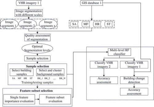
Figure 1 shows the flowchart of the major components of the proposed method in this study. Our approach requires VHR imagery and GIS data consisting of four types of buildings. The workflow of the proposed method is as follows: (1) segmenting the VHR imagery at multiple scales, and selecting the optimal scale for each type of buildings with the aid of GIS data, (2) choosing both building and background samples with the aid of GIS data, (3) choosing optimal feature subsets with CFS method, and (4) classifying image segments with selected samples and feature subsets.

Figure 1. The overall process for building extraction and change detection.

2.1. Typology of building categories

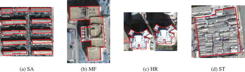
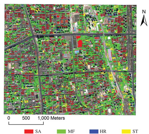
As buildings in urban areas vary greatly in appearances, such as color, size, shape, and texture, it is difficult to extract all types of buildings from VHR imagery using the same SSPs, which will result in low classification accuracy. By analyzing characteristics of buildings on the VHR imagery and GIS data, and summarizing existing building semantic classification systems (Du, Zhang, and Zhang 2015; Lu et al. 2014), four building types are identified (Figure 2): single-apartment (SA) buildings, multi-function (MF) buildings, high-rising (HR) buildings, and shantytown (ST) buildings.

• SA buildings (Figure 2(a)) usually have flat or gable roofs with rectangular shapes and a large ratio of length to width. Their heights are between three and eight stories.

• MF buildings (Figure 2(b)) are composed of several buildings with different appearances. When generating GIS layer of buildings, buildings with the same functions or belonging to the same institution tend to be represented as one polygon. These kind of buildings usually have large heterogeneity.

• HR buildings (Figure 2(c)) can be residential or commercial buildings. They are usually bright in color and have large contrast with their surroundings. HR buildings often have equal length and width, but complex shapes.

• ST buildings (Figure 2(d)) are represented by large polygons in the GIS layer. They are usually residential buildings and mainly for poor people and middle classes. The height of ST building is low and the area is large. Besides, they have rich textures on the VHR imagery.

Figure 2. Four types of buildings: (a) Single-apartment (SA); (b) Multi-function building (MF); (c) High-rise building (HR); (d) Shantytown (ST).

The type of each building polygon is predetermined and stored in the attribute of GIS data.

2.2. Selection of optimal segmentation scales

The multi-resolution segmentation (MRS) algorithm is used to segment VHR imagery in this study. This algorithm is a bottom-up technique which starts with pixels and merges the adjacent segments until a certain heterogeneity threshold is reached (Benz et al. 2004). The heterogeneity is determined by three parameters: scale, color/shape, and compactness/smoothness. Among the three parameters, the color/shape weights and the compactness/smoothness weights are usually set as default values, i.e., 0.9/0.1 and 0.5/0.5, respectively. However, the optimal scales are difficult to be determined, as they vary over different images, and different types of buildings even in the same image. Meanwhile, the scale parameters directly determine the segmentation quality and the precision of information extraction (Ma et al. 2015; Liu and Xia 2010; Ming et al. 2015). To identify the optimal segmentation scales, a series of segmentations (larger than four) with discrete scale parameters are carried out, and then the optimal segmentation scales are determined by evaluating the quality of segmentations at all scales.

In this study, existing GIS-building polygons are used to evaluate the segmentation quality. The optimal segmentation scale of each type is determined individually. After segmenting the VHR imagery, segments are obtained and compared with each type of GIS-building polygons to evaluate the segmentation performance. Three metrics are used to evaluate how segments are consistent with the polygons, including over-segmentation (OSeg), under-segmentation (USeg), and root mean square (RMS) (Clinton et al. 2010). Let be the set of segments, and be the set of polygons. For each and , if satisfies Equation (1), it will be regarded as a correspondence of , and added to a set .

(1)

where is the area of , and the overlapping area between and . The threshold 0.5 is recommended by Weidner (2008).

By using Equation (1), the correspondences between segments and polygons are determined. For a segment and its corresponding polygon , the three metrics are computed as:

(2)

Both and can measure how image segment fits with GIS polygon , and integrates the two measurements into one. , , and are the averages of all , , and (), and can measure the fitting degree of all the image segments to GIS polygons. The values of , , and range from 0 to 1. , , and means the best segmentation, which can hardly be achieved. In practice, the imagery is either over- or under-segmented. The smaller these three values, the better the segmentation results. For each type of buildings, the GIS polygons of this type are compared with the segments at each segmentation level individually, and the scale with the lowest evaluation metrics is considered as the optimal segmentation scale. In so doing, the optimal segmentation scales of the four types of buildings are identified separately.

2.3. Selection of samples assisted by GIS data

The previous section finds the optimal segmentation scales of the four types of buildings and generates corresponding image segments. This section attempts to select samples from these segments. Existing studies have demonstrated that the supervised classification highly depends on the quality of samples. Therefore, an efficient method is required to select a large number of samples. The samples should reflect the distributions of features on different classes, and the number should be in proportion to the total number of segments in each category. Traditional approaches often manually select samples, which obviously cannot satisfy the above requirements. In this study, GIS data are employed to facilitate sample selection.

2.3.1. Selection of building samples

For each type of buildings, its corresponding GIS layer is superposed on the optimal segmentation level to select initial building candidates. The overlapping degrees between the segments and polygons are computed (Equation (3)). For a segment , if its overlapping degrees with polygons are larger than a threshold (usually set as 0.6), it will be selected as a candidate.

(3)

where is the overlapping degree of , a GIS polygon, and the set of GIS polygons of one type.

In so doing, building candidate sets of four types ( = 1,2,3,4 corresponding to SA, MF, HR, and ST) can be obtained. Not all the segments in are selected as building samples. As VHR imagery and GIS data are acquired at different time, buildings might change. A confirmation procedure is performed to verify if the chosen segments represent real buildings. For the first three types of buildings (SA, MF, and HR), shadows are useful to verify the existence of buildings. As ST buildings are usually low, shadows are not significant. To eliminate the possible changes of ST buildings, the Built-Up Areas Index (BAI) (Bouziani, Goïta, and He 2010b) is used.

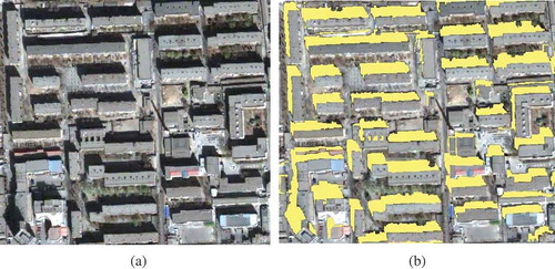
First, shadow segments at the four levels are extracted. Because shadows usually have low brightness and large spectral differences at different bands, they can be extracted by using two spectral features: Brightness and Max.diff (Guo, Du, and Zhang 2013). Figure 3 illustrates a small Quickbird imagery and the extracted shadow segments.

(4)

(5)

Figure 3. (a) Quickbird imagery, and (b) the detected shadow segments.

where are average spectral values of a segment at red, green, blue, near-infrared and panchromatic bands.

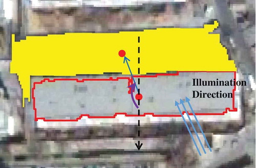
Second, shadow segments are used to confirm building candidates. As to each candidate segment in , the neighboring shadow segments on the image are found. The azimuths of lines which start from the building segment’s centroid and end at the centroids of shadow segments are calculated, and then compared with the sun’s azimuth. If one of the computed azimuths has a small discrepancy with the sun’s azimuth, this building segment is preserved. Through trial and error, the angle threshold is set as 20°. Figure 4 shows an example of the azimuth between a building segment and a neighboring shadow segment.

Figure 4. The azimuth between a building and a shadow segment.

As to ST buildings, they cannot be confirmed by shadow characteristics. Instead, the BAI index is employed (Equation (6)). As building materials are sensitive to blue and near-infrared bands, BAI is efficient in detecting built-up areas (Bouziani, Goïta, and He 2010b). In order to eliminate possible transitions and incorrectly selected samples, BAI of each segment in ST building candidate set () is computed and analyzed. Assuming that the BAIs of building segments follow a normal distribution, then the nonbuilding segments may fall within the two tails of the normal distribution. Therefore, only segments satisfying Equation (7) are selected as building samples.

(6)

(7)

where is the BAI value of the -th segment in , the average BAI value of all segments in , and the standard BAI value of all segments in .

Samples of four types of buildings are selected from the corresponding segmentation levels, and a stratified sampling method (Padilla, Stehman, and Chuvieco 2014) is conducted to randomly select 50% of samples as training samples, and the rest 50% for testing (recommended by Ma et al. 2015; Li, Dong, and Zhang 2014b).

2.3.2. Selection of background samples

The background samples are selected from the segments at the finest scale of the above four determined optimal scales to avoid mixture of background objects (i.e., a single segment contains different types of objects). The selection includes three steps: initial selection, background confirmation, and background clustering.

First, GIS polygons are used for initial selection of background samples. If a segment has a small overlapping degree (usually less than 0.05) with GIS polygons, it will be considered as a background candidate. In so doing, a background candidate set is obtained at the first step.

The second step is background confirmation. In this step, extracted shadows are employed to remove possible transitions from background to buildings. As to each shadow segment, its neighboring segments in are considered. If the azimuth of a line starting from the shadow segment’s centroid and ending at the centroid of a candidate background segment is close to the sun’s azimuth (smaller than 20°), the candidate segment should be removed. As the transition from background to ST building rarely happens in cities, this case can be ignored. In so doing, the background sample set is refined.

The third step is background clustering. As background samples represent different classes of objects and vary greatly in characteristics, it is necessary to group them into different clusters. In this study, Expectation and Maximization (EM) clustering algorithm is employed to perform this task such that background segments in the same cluster will have similar characteristics. The EM algorithm is an iterative method for finding maximum likelihood estimates of parameters (Yang, Lai, and Lin 2012). The EM iteration alternates between the E-step and the M-step, in which the E-step creates a function using the current estimates, and the M-step computes the parameters maximizing the expected likelihood found in the E-step. However, the EM algorithm requires the number of clusters as a priori (Yang, Lai, and Lin 2012). To find appropriate number of clusters, a series of experiments with different numbers are conducted, and the prior number is selected according to the classification accuracy which will be introduced in Section 3.4.

After EM clustering, the background samples are grouped into clusters. The stratified sampling method (Padilla, Stehman, and Chuvieco 2014) is employed to select training and test sets. For each background cluster, 50% samples are randomly selected for training and testing, respectively.

2.4. Selection of optimal features

Compared to pixel-based methods, GEOBIA generates hundreds of features including spectral, geometric, and textural ones. It is impossible to include all these features as it will take a lot of computational loads. A total number of 33 commonly used features are listed in Table 1. These features can be divided into three groups: (A) 13 spectral features –, (B) 12 geometric features -, and (C) 8 textural features –. For each segment, the above 33 features are calculated by using eCognition software. However, not all these features are efficient in distinguishing building segments from others. Besides, some of these features are highly correlated. Accordingly, feature selection is very important. In this study, the method of feature selection contains two components: a single feature importance evaluation and a feature subset evaluation method.

Table 1. The commonly used features based on image segments.

Types	Codes	Indices	Description
Group A: Spectrum (13)		[Mean]	Average spectral values on blue, green, red, near-infrared and pan band
		[Std. dev]	Standard deviation on blue, green, red, near-infrared and pan band
		[Max. diff]	Maximum difference of all band values
		[NDVI]	Normalized difference vegetation index
		[BAI]	Built-up area index
Group B: Geometry (12)		[Area_pxl]	Number of pixels within image objects
		[Border_ind]	The ratio between the border lengths of a building and the smallest enclosing rectangle
		[Border_len]	Number of pixels in the inner and outer borders
		[Compactness]	The ratio of the product of length and width to the area of an image object
		[Length_pxl]	The length of the skeleton line of an image object
		[LengthWidth]	The length-to-width ratio of an image object
		[Main_dir]	The direction of the eigenvector belonging to the larger of the two eigenvalues
		[Elliptic_F]	How well an image object fits into an ellipsoid of similar size and proportions
		[Rectangular_F]	How well an image object fits into a rectangle of similar size and proportions
		[Roundness]	How similar an image object is to an ellipse
		[Shape_index]	The smoothness of an image object border
		[Width_pxl]	The length of the line which is perpendicular to the skeleton line
Group C: Texture (8)		[GLCM_Ang_2]
		[GLCM_Con]
		[GLCM_Diss]
		[GLCM_Entro]
		[GLCM_Hom]
		[GLCM_Mean]
		[GLCM_Stdv]
		[GLCM_Corrle]

Note: and refer to the row and column, the normalized value in the cell .

The single feature importance evaluation method is used to assess the contribution of each feature in classifying segments. The gain ratio presented by Quinlan (1996) has been proven to be a good metric and can be computed by Equation (8):

(8)

where is a feature, the gain value of , and the split information of . The calculation of and can be referred to Quinlan (1996). The larger the GainRatio value, the more important the feature.

However, not all the top ranking features are selected. This is because some top ranking ones are highly correlated with each other. In this study, the best-first search (BFS) strategy and CFS method (Hall and Holmes 2003) are combined to select the optimal feature subset. First, all features are ranked based on their gain ratio scores and added to a feature subset in sequence. The quality of the feature subset is measured by CFS, which considers the ability of each feature with the degree of redundancy among them (Huang, Yang, and Chuang 2008):

(9)

where refers to the score of a feature subset including features, the class, and the feature, the average feature-class correlation, and the average feature-feature correlation. The features will not be added to the feature subset when evaluation scores of the feature subset do not increase anymore.

This procedure is performed on Weka 3.6.13 to obtain the optimal feature subset, which is further used in object-based classification.

2.5. Object-based building classification with multilevel random forest

When samples and optimal feature subsets are obtained, the RF algorithm is used to classify the segments. The RF has been widely used in remote sensing classification and object extraction, and proved to be a successful classifier (Ham et al. 2005; Pal 2005). RF is composed of a number of decision trees, with each one being trained independently, and the final prediction is determined by the vote of all decision trees. The construction of each decision tree is as follows: (1) a subset of samples are randomly chosen by using the Bootstrap sampling methods, (2) a subset of features are randomly selected for each node, (3) at each node, the optimal features and thresholds are determined by finding the largest information gain and used to split each node into two sub-nodes, and (4) the splitting process continues until the tree reaches the maximum depth or all the samples in the node belong to the same class. Two main parameters are required in RF method. The first is the number of trees, which is set to a relatively large fixed number of 200, and a larger number would not significantly improve the accuracy. The second parameter is the number of features to split the nodes, which is usually recommended to be the square root of the total number of input features (Ham et al. 2005).

In this study, the trained RF classifier is used to classify segments from hierarchical image segmentation levels, and extract building segments from the four segmentation levels. However, the traditional RF classifier can only classify segments at one segmentation level one time. A segment is assigned to one class by RF classifier while its super- and subsegments might be assigned to different classes. Therefore, traditional RF cannot classify multilevel image segments.

In order to overcome this drawback, the traditional RF classifier is adapted to a multilevel RF classifier. First, a hierarchical structure is formed by the four optimal segmentation levels selected in Section 2.2, the relations between segments in different levels are built (i.e., the super- and subsegments can be found). Second, segments at each segmentation level are classified by RF classifier. Instead of directly assigning a class to a segment, the RF classifier assigns a probability that a segment belongs to a certain type of class. The probability (Equation (10)) is in proportion to the number of the votes in RF.

(10)

where the probability of the -th category with , the number of votes of the -th category, the total number of trees in the RF classifier, and the number of categories. In the third step, the probabilities of segments at each coarse segmentation levels are added to their sub-objects at the finest segmentation level, based on which the final classification results are determined. A segment at the finest segmentation level is assigned to the class with the highest probability.

3. Experiments

Two datasets are employed in this study. Dataset 1 is used to mine information for building extraction including optimal segmentation scales (Section 3.2) and optimal feature subsets (Section 3.3). Meanwhile, the number of background clusters is analyzed and the optimal one is selected according to the results of accuracy assessment (Section 3.4). The mined information is further used to classify VHR images in Dataset 1 (Section 3.5) and Dataset 2 (Section 3.6). Changes of buildings in Dataset 1 are also detected by comparing the extracted buildings from the VHR imagery with GIS data (Section 3.6).

3.1. Study areas and data description

The study area is located in urban city of Beijing, the capital of China. Buildings in this area are densely distributed.

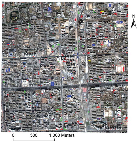
Dataset 1 contains a Quickbird imagery (Figure 5(a)) and corresponding GIS data consisting of four types of buildings (Figure 5(b)). The Quickbird image is composed of four multispectral bands and one panchromatic band, and all bands are resampled to 0.61 m. The Quickbird imagery was acquired at a local time on 14 March 2008, while the GIS data were produced in 2004. It covers the same area and contains boundaries of buildings. The two data sources have been geo-referenced and the geometrical discrepancies have been reduced to the minimum. Dataset 1 covers an area of 3055  × 3150  and consists of approximately 2930 buildings. It is worth mentioning that building changes may exist between the two data sources due to their different acquisition time.

Figure 5. Study area and test datasets. (a) Quickbird image of Dataset 1; (b) GIS data including four types of buildings in Dataset 1; and (c) Quickbird image of Dataset 2.

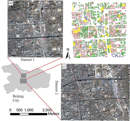
Dataset 2 includes only a Quickbird imagery acquired on the same day (14 March 2008) with the image in Dataset 1, but at different locations. The Dataset 2 covers an area of 3815  × 3185 .

3.2. Results of optimal segmentation scales

A number of segmentation experiments are conducted on Quickbird imagery in Dataset 1 with different scale parameters. The scale parameters begin at 30 and end at 200, with increments of 10. We do not try parameters below 30 or above 200, because according to visual interpretation, buildings are obviously over- or under-segmented at these scales. The performance of segmentation results at 18 scales is evaluated by using GIS polygons. For each type of buildings, the quantitative results at different scales are shown in Table 2.

Table 2. Quantitative results of segmentations at different scales in terms of four types of buildings.

	SA			MF			HR			ST
Scale	OSeg	USeg	RMS	OSeg	USeg	RMS	OSeg	USeg	RMS	OSeg	USeg	RMS
30	0.833	0.153	0.61	0.938	0.127	0.678	0.921	0.13	0.667	0.982	0.068	0.701
40	0.746	0.176	0.558	0.909	0.145	0.661	0.882	0.147	0.643	0.972	0.083	0.696
50	0.67	0.195	0.516	0.879	0.156	0.642	0.842	0.175	0.623	0.961	0.096	0.69
60	0.599	0.221	0.482	0.85	0.167	0.625	0.803	0.197	0.605	0.95	0.103	0.683
70	0.538	0.249	0.458	0.819	0.182	0.61	0.765	0.216	0.589	0.94	0.121	0.678
80	0.483	0.285	0.444	0.789	0.195	0.594	0.724	0.256	0.579	0.927	0.13	0.672
90	0.438	0.317	0.435	0.761	0.21	0.583	0.687	0.288	0.572	0.904	0.149	0.661
100	0.404	0.353	0.434	0.728	0.236	0.573	0.65	0.327	0.568	0.891	0.156	0.653
110	0.374	0.388	0.438	0.697	0.263	0.566	0.613	0.355	0.56	0.877	0.16	0.645
120	0.349	0.425	0.446	0.666	0.287	0.556	0.584	0.377	0.555	0.858	0.179	0.641
130	0.32	0.472	0.458	0.633	0.321	0.557	0.559	0.404	0.553	0.848	0.194	0.639
140	0.299	0.514	0.472	0.601	0.356	0.559	0.531	0.43	0.551	0.832	0.206	0.632
150	0.284	0.554	0.489	0.575	0.394	0.559	0.506	0.455	0.555	0.801	0.235	0.623
160	0.269	0.588	0.503	0.545	0.427	0.56	0.48	0.481	0.554	0.772	0.262	0.615
170	0.255	0.623	0.518	0.525	0.449	0.562	0.461	0.503	0.557	0.749	0.292	0.612
180	0.244	0.65	0.531	0.5	0.488	0.566	0.44	0.52	0.554	0.731	0.317	0.61
190	0.234	0.673	0.541	0.471	0.516	0.566	0.419	0.544	0.555	0.725	0.326	0.611
200	0.223	0.703	0.555	0.445	0.548	0.57	0.402	0.574	0.564	0.705	0.348	0.612

As shown in Table 2, as segmentation scales increase, the values of increase, while the values of decrease. This accords with our knowledge that a small segmentation scale will result in over-segmentation, while a large segmentation scale will result in under-segmentation. All the RMS values have very similar trend, that is, as scales increase, the RMS values first decrease and then increase. The optimal segmentation scales are selected at the points with lowest RMS values. Therefore, the optimal scales for SA, MF, HR, and ST are 100, 120, 140, and 180, respectively. Segmentations at these four scales form a hierarchical structure.

3.3. Results of optimal features

After the four optimal segmentation scales being obtained, samples of the four types of buildings can be selected at their corresponding segmentation scales individually (Section 2.3.1). Background samples are selected at the scale of 100, and divided into clusters (Section 2.3.2). A total of approximately 14,000 samples are selected. In terms of different numbers of background clusters (), the optimal feature subsets are selected (Section 2.4) and reported in Table 3. The optimal feature subsets vary among different values. For the 12 (N = 1 ~ 12) different cases, some features can be selected with large chances, including Mean_blue, NDVI, BAI, Area_pxl, Border_ind, Border_len, Compactness, Length_pxl, LengthWidth, Shape_index, Width_pxl, GLCM_Ang_2, GLCM_Con, GLCM_Entro, and GLCM_Hom. Meanwhile, some features are most likely excluded in the optimal feature subsets, such as Std_nir, Max.diff, Main_dir, GLCM_Diss, and GLCM_Stdv, indicating that these features might not be useful in distinguishing different classes. Among all the 33 features, geometric ones are more likely included in the optimal feature subsets.

Table 3. The optimal feature subset in terms of different numbers of background clusters.

		Number of background clusters ()
Code	Feature	1	2	3	4	5	6	7	8	9	10	11	12
	[Mean_blue]	√	√	√	√	√	√	√	√	√	√	√	√
	[Mean_green]	×	√	×	√	√	×	×	×	×	×	√	×
	[Mean_red]	×	×	×	√	√	×	×	×	×	×	×	×
	[Mean_nir]	×	×	×	×	×	√	√	√	×	√	×	×
	[Mean_pan]	×	×	×	×	×	×	√	×	√	×	√	√
	[Std_blue]	×	√	×	×	√	×	√	×	√	×	√	×
	[Std_green]	×	×	×	√	×	√	×	√	×	√	×	√
	[Std_red]	×	×	×	×	√	×	√	√	×	√	√	√
	[Std_nir]	×	×	×	×	×	×	×	×	×	×	×	×
	[Std_pan]	√	√	√	√	×	√	×	×	√	×	√	×
	[Max.diff]	√	×	×	×	×	×	×	×	×	×	×	×
	[NDVI]	√	√	√	√	√	√	√	√	√	√	√	√
	[BAI]	√	×	×	√	×	√	√	√	√	√	√	√
	[Area_pxl]	×	√	√	√	√	√	√	√	√	√	√	√
	[Border_ind]	√	√	√	√	√	√	√	√	√	√	√	√
	[Border_len]	×	√	√	√	√	√	√	√	√	√	√	√
	[Compactness]	×	√	√	√	√	√	√	√	√	√	√	√
	[Length_pxl]	×	√	√	√	√	√	√	√	√	√	√	√
	[LengthWidth]	√	×	×	×	√	√	√	√	√	√	√	√
	[Main_dir]	√	√	×	×	×	×	×	×	×	×	×	×
	[Elliptic_F]	×	×	×	×	×	×	×	√	√	√	×	√
	[Rectangular_F]	×	×	×	×	×	√	√	√	√	√	√	√
	[Roundness]	×	×	×	×	√	×	×	√	×	×	√	×
	[Shape_index]	×	×	√	√	√	√	√	√	√	√	√	√
	[Width_pxl]	×	√	√	√	√	√	√	√	√	√	√	√
	[GLCM_Ang_2]	×	√	√	√	√	√	√	√	√	√	√	√
	[GLCM_Con]	√	√	×	×	√	√	√	√	√	√	√	√
	[GLCM_Diss]	×	×	×	×	√	×	×	×	√	×	×	×
	[GLCM_Entro]	√	√	√	√	√	√	√	√	√	√	√	√
	[GLCM_Hom]	√	√	√	√	√	√	√	√	√	√	√	√
	[GLCM_Mean]	×	√	×	√	√	×	√	√	×	×	√	√
	[GLCM_Stdv]	×	×	×	×	√	×	×	×	×	×	×	×
	[GLCM_Corrle]	×	√	√	√	√	√	×	√	×	√	√	√

To further analyze the contributions of the input features to classification, the gain ratio value of each feature is computed. Due to the space limitation, Figure 6 only shows the gain ratio values of all features when and .

Figure 6. Contribution of each feature and the results of feature selection at (a) and (b). Note that the red bars represent the selected features in the optimal feature subsets.

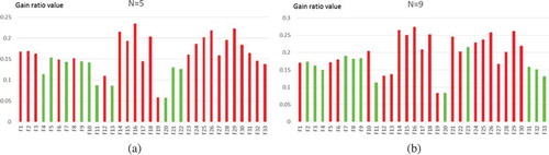
As shown in Figure 6, the optimal subset consists of 23 features for and 21 features for . Note that not all the top 23 or 21 features with large gain ratios are selected. For example, when , the feature has a smaller gain ratio than , but is selected into the optimal subset while not. The reason is that there is a strong correlation between and the features that are already included in the subset. The contribution of a feature is normalized by dividing its gain ratio value by the sum of all features’ gain ratio values. When , the computed contributions of spectral, geometric, and textural features are 34.75%, 37.34%, and 27.91%, respectively. While , the contributions are 34.42%, 40.78%, and 24.80%, respectively. The quantitative results indicate that the geometric features contribute the most.

3.4. Parameter analysis of the number of background clusters

To better distinguish buildings from nonbuildings, background samples are divided into different clusters (Section 2.3.2), thus the influences of different numbers (1 ~ 12) of background clusters on classification results need to be analyzed. With different numbers of background clusters, the selected samples in each class are different, and optimal feature subsets are selected accordingly (Section 3.3). Based on trained samples and chosen features, RF classifier is trained and then used to classify test samples, which can produce a confusion matrix (Table 4). The performance of classification is evaluated based on the confusion matrix.

Table 4. Confusion matrix of object-based classification.

	Classified
Real class	SA	MF	HR	ST	BK_1	BK_2	…	BK_N
SA							…
MF							…
HR							…
ST							…
BK_1							…
BK_2							…
…	…	…	…	…	…	…	…	…
BK_N							…

Note: Note that denotes the number of segments in -th row and -th column. BK_1, BK_2 … BK_N are all background categories.

To evaluate classification accuracies of four types of buildings, the confusion matrix is divided into four parts:

True Positive (TP): the upper-left part of the matrix.

(11)

False Negative (FN): the upper-right part of the matrix.

(12)

False Positive (FP): the lower-left part of the matrix.

(13)

True Negative (TN): the lower-right part of the matrix.

(14)

denotes the number of segments in -th row and -th column in Table 4. Based on these four parts, three indicators are defined to evaluate the performance: Precision, Recall, and score (Equation (15)).

(15)

Both and measure the performance of building classification. score integrates and into one measurement. The accuracy assessment facilitates to analyze the effects of the number of background clusters and choose an appropriate number of background clusters. Figure 7 shows the accuracy assessment results in terms of different numbers of background clusters.

Figure 7. Accuracy assessments of building classification using random forest in terms of different numbers of background clusters.

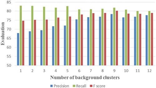
As seen in Figure 7, the Recall values remain steady (80.17–83.01%) among 12 different numbers of clusters, which means that increasing the number of background clusters does not improve the Recall accuracy significantly. However, the Precision values vary according to the number of background clusters. Results of Precision demonstrate the necessity of dividing background into multiple clusters. With the number of background clusters increasing, the Precision first rises and reaches the maximum at . It then drops at and remains at a stable level afterward. This phenomenon can be explained as follows. As the number of background clusters increases, the heterogeneity in each background class decreases. This will help RF to distinguish each background cluster from buildings. Therefore, building misclassification will accordingly decrease. However, as the number of background clusters continues to rise, the accuracy will not increase anymore. The score has a similar trend with the Recall. It first increases and then decreases, and the maximum score (80.18%) is obtained at . Accordingly, is adopted as the number of background clusters and used in the subsequent analysis.

3.5. Dataset 1: change detection of buildings

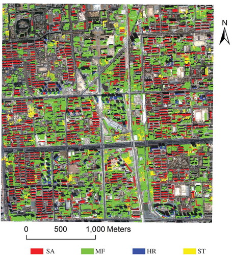
Based on the previous analysis, the optimal segmentation scales for the four types of buildings are 100, 120, 140, and 180, respectively. Building samples are selected from the segments at the four segmentation scales, respectively, and background samples are selected from the segments at segmentation scale of 100. The background samples are grouped into nine clusters. An optimal feature subset including 21 features is selected. Using the selected samples and features, a multilevel RF classifier (Section 2.5) is trained and employed to classify the VHR imagery in Dataset 1.

Figure 8 shows the extracted buildings from VHR imagery in Dataset 1. In total, 5548 building segments are extracted from the VHR imagery, including 1618 SA, 3527 MF, 243 HR, and 160 ST segments, respectively.

Figure 8. Building extraction from VHR imagery in Dataset 1.

As mentioned in Section 3.1, the imagery and GIS data were acquired at different time, and building changes may happen. To detect the changes, the extracted buildings are compared with GIS data. If an extracted building segment has more than 60% overlapping degree with GIS polygons, it will be considered as unchanged; otherwise, a new building. Likewise, if a GIS-building polygon has less than 60% overlapping degree with extracted building segments, it will be considered as a destroyed building. The neighboring segments detected as changed are merged and regarded as one changed building. Figure 9 shows the detected changes between GIS data and VHR imagery, and every changed building is visually inspected. In addition, the undetected changes of buildings are also checked in the whole the study area. The number of correctly detected, incorrectly detected and undetected changes of buildings (including both newly increased and destroyed buildings) are counted and illustrated in Table 5. According to Table 5, a total of 164 buildings are detected newly increased from GIS data to VHR imagery, in which 131 buildings are correctly detected, and 33 are false alarms. And 12 newly increased buildings are undetected. A total of 89 building polygons are detected as destroyed from GIS data to VHR imagery, in which 72 polygons are correct, and 17 are false alarms. And 9 destroyed buildings are undetected. Therefore, the precision of detected increased buildings is 79.9%, the false alarm ratio is 20.1%, while the omission error is 8.4%. The precision of detected destroyed buildings is 80.9%, the false alarm ratio is 19.1%, while the omission error is 11.3%.

Table 5. Quantitative results of change detection from GIS data to VHR imagery.

	Corrected detection	False alarms	Missed detection
Newly increased	131	33	12
Destroyed	72	17	9

Figure 9. Results of change detection from GIS data to VHR imagery. Red polygons represent correct detections of increased buildings from GIS data to VHR imagery, green false alarms of increased buildings, blue correctly detected destroyed buildings, and yellow false alarms of destroyed buildings.

Although there are some false alarms and undetected changes, the overall results by the proposed method are good. The false alarm ratio is a little larger than omission error for both newly increased and destroyed buildings. False alarms of newly increased buildings are usually concrete playground or parking lots, which have very similar features with buildings. There are also some confusions occurring between MF buildings and roads. As to the destroyed buildings, some of them do not really disappear but are occluded by shadows or trees on VHR images, causing false alarms.

3.6. Dataset 2: building extraction results

As the VHR imagery in Dataset 2 is very similar to that in Dataset 1, the mined information from Dataset 1 is used to classify VHR imagery in Dataset 2. First, the imagery is segmented with four scales (i.e., 100, 120, 140, and 180) to form a hierarchical structure. Then, the multilevel RF classifier is employed to classify hierarchical segments. The extracted buildings are shown in Figure 10. As can be seen, most buildings are successfully extracted.

Figure 10. Building extraction from Dataset 2.

Aside from visual illustration, the results of building extraction in Dataset 2 are also evaluated quantitatively. The results are compared with a standard building map manually delineated by human experts. The quantitative evaluation is performed at both pixel and object levels. The three metrics, Precision, Recall, and score, are used for both pixel- and object-based evaluation. The quantitative results are revealed in Table 6. For pixel-based evaluation, the Precision, Recall, and score are 83.0%, 80.1%, and 81.5%, respectively. As to object-based performance, the Precision, Recall, and score are 80.0%, 82.3%, and 81.1%, respectively. These results demonstrate that the number of the missed building pixels exceeds that of over-classified building pixels. However, the number of the missed building segments is less than the number of over-classified building segments. In general, the results are satisfactory, especially on such a diverse and complicated area.

Table 6. Pixel- and object-based accuracies of extracted buildings on Dataset 2.

Model	Precision (%)	Recall (%)	score (%)
Pixel-based evaluation	83.0	80.1	81.5
Object-based evaluation	80.0	82.3	81.1

4. Discussions

Building extraction and change detection from VHR images are two important but challenging tasks due to the complexity of buildings. GEOBIA methods are specially designed for processing VHR images. However, there are some unresolved issues for GEOBIA methods, including identification of segmentation scales, selection of effective features, and sample selection. It is difficult to solve these issues by solely using VHR images, thus GIS data are incorporated in this study. A parameter mining method is proposed by combining VHR imagery and GIS data to extract buildings and detect changes. The proposed method has the following merits.

1. Buildings are divided into different subcategories. In urban environment, buildings are usually very complexed and their characteristics vary greatly. However, most existing methods (Bouziani, Goita, and He 2010a; Lee, Shan, and Bethel 2003) do not distinguish different types of buildings and adopt the same rules and features to extract all buildings, which leads to low classification accuracy. In this study, buildings are divided into four types: SA, MF, HR, and ST, and each type has its own segmentation scale and classification ruleset.

2. GIS data help to identify optimal segmentation scales. The quality of segmentation is evaluated by GIS data, and the optimal segmentation scale of each type of buildings is chosen from 18 discrete scales (30–200). The proposed method excels unsupervised methods (Kim, Madden, and Warner 2008; Drǎguţ, Tiede, and Levick 2010; Johnson and Xie 2011) and supervised methods (Ma et al. 2015) in considering not only image perspective but also actual geographic objects.

3. GIS data play an important role in sample selection. A large number (approximately 14,000) of samples of different types are chosen at different segmentation levels. Such a large number is difficult to be achieved by manual selection.

4. GIS data indirectly help select the optimal feature subset from 33 commonly used features. The optimal feature subset can maximally distinguish different classes, and avoid high correlations between similar features.

For Dataset 1, the extracted buildings from VHR imagery are compared with GIS data to detect changes. The false alarm ratio of the increased buildings is 20.1%, while the omission error is 8.4%. As to the destroyed buildings, the false alarm ratio is 19.1%, while the omission error is 11.3%. For Dataset 2, the pixel- and object-based scores of building extraction are 81.5% and 81.1%. The results show that the false alarms of increased buildings come from (1) concrete playgrounds or parking lots as they have very similar features with buildings, and (2) the confusions between MF buildings and roads. Some buildings on VHR images are misclassified because they are occluded by shadows or trees.

Although the proposed method produces good results of change detection and building extraction for the test sites, there are also some limitations. First, LIDAR data can provide height information, thus the confusion between buildings and other classes can easily be removed, and the occlusions can be identified by using LIDAR data. In the future, we will study on fusing VHR imagery, GIS and LIDAR data to improve accuracies. Second, the category of each building in GIS data is available in this study. However, sometimes it is difficult to obtain such information, thus an automatic semantic classification method is required. Third, the boundaries of extracted buildings are irregular. We plan to improve boundaries of buildings by conducting boundary regularization after building extraction. Fourth, accuracy assessment of building extraction and change detection are based on the overlapping degree between extracted buildings and reference polygons. However, the shape difference between the two are not evaluated. In the future, we will study on evaluating the shape accuracy of extracted buildings.

5. Conclusions

This study proposed a parameter mining approach to combine VHR imagery and GIS data to learn knowledge of building extraction, such as segmentation scales, number of background clusters, and the optimal feature subset. This study considers the inconsistencies between VHR imagery and GIS data, and fully exploits the use of GIS data. The GIS data are first used to determine the segmentation scales by comparing three quantitative metrics at different segmentation levels, and then help automatically select both building and nonbuilding samples. Besides, the GIS data indirectly help to choose optimal feature subsets by using CFS, and serve as reference data in change detection. Our study has two main objectives: (1) mining parameter information for extracting buildings from other datasets, and (2) detecting changes of buildings between VHR images and GIS data.

The proposed approach was conducted on two datasets: Dataset 1 and Dataset 2. Knowledge of buildings was first learned from Dataset 1 comprising a Quickbird image and GIS data, and then used to extract buildings from images in both Dataset 1 and 2. Extracted buildings from Dataset 1 were further compared with GIS data to detect changes. Results were evaluated quantitatively and demonstrated that the proposed method extracted buildings and detected changes with a high success rate.

The proposed approach was primarily designed for buildings. However, it would also be possible and interesting to adapt it to other urban objects. This research has two immediate applications. The first one is database updating and change detection in urban environments. The second one is large-area mapping. Nevertheless, there are some limitations of the proposed method. Our future work will focus on reducing the limitations.

Acknowledgments

The work presented in this paper was supported by the National Natural Science Foundation of China under grant 41471315.

Disclosure statement

No potential conflict of interest was reported by the authors.

Additional information

Funding

This work was supported by the National Natural Science Foundation of China: [Grant Number 41471315].

References

- Almuallim, H., and T. G. Dietterich. 1991. “Learning with Many Irrelevant Features.” Proceedings of the Ninth National Conference on Artificial Intelligence 2: 547–552.
- Benz, U. C., P. Hofmann, G. Willhauck, I. Lingenfelder, and M. Heynen. 2004. “Multi-Resolution, Object-Oriented Fuzzy Analysis of Remote Sensing Data for GIS-Ready Information.” ISPRS Journal of Photogrammetry and Remote Sensing 58: 239–258. doi:10.1016/j.isprsjprs.2003.10.002.
- Bouziani, M., K. Goita, and D. He. 2010a. “Rule-Based Classification of a Very High Resolution Image in an Urban Environment Using Multispectral Segmentation Guided by Cartographic Data.” IEEE Transactions on Geoscience and Remote Sensing 8 (48): 3198–3211.
- Bouziani, M., K. Goïta, and D. He. 2010b. “Automatic Change Detection of Buildings in Urban Environment from Very High Spatial Resolution Images Using Existing Geodatabase and Prior Knowledge.” ISPRS Journal of Photogrammetry and Remote Sensing 65: 143–153. doi:10.1016/j.isprsjprs.2009.10.002.
- Clinton, N., A. Holt, J. Scarborough, L. Yan, and P. Gong. 2010. “Accuracy Assessment Measures for Object-Based Image Segmentation Goodness.” Photogrammetric Engineering & Remote Sensing 76: 289–299. doi:10.14358/PERS.76.3.289.
- Dong, L., and J. Shan. 2013. “A Comprehensive Review of Earthquake-Induced Building Damage Detection with Remote Sensing Techniques.” ISPRS Journal of Photogrammetry and Remote Sensing 84: 85–99. doi:10.1016/j.isprsjprs.2013.06.011.
- Drăguţ, L., O. Csillik, C. Eisank, and D. Tiede. 2014. “Automated Parameterisation for Multi-Scale Image Segmentation on Multiple Layers.” ISPRS Journal of Photogrammetry and Remote Sensing88: 119–127. doi:10.1016/j.isprsjprs.2013.11.018.
- Drǎguţ, L., D. Tiede, and S. Levick. 2010. “ESP: A Tool to Estimate Scale Parameter for Multiresolution Image Segmentation of Remotely Sensed Data.” International Journal of Geographical Information Science 24 (6): 859–871. doi:10.1080/13658810903174803.
- Du, S., Z. Guo, W. Wang, L. Guo, and J. Nie. 2016. “A Comparative Study of the Segmentation of Weighted Aggregation and Multiresolution Segmentation.” GIScience & Remote Sensing 53 (5): 651–670. doi:10.1080/15481603.2016.1215769.
- Du, S., F. Zhang, and X. Zhang. 2015. “Semantic Classification of Urban Buildings Combining VHR Image and GIS Data: An Improved Random Forest Approach.” ISPRS Journal of Photogrammetry and Remote Sensing 105: 107–119. doi:10.1016/j.isprsjprs.2015.03.011.
- Gao, L., T. Li, L. Yao, and F. Wen. 2014. “Research and Application of Data Mining Feature Selection Based on Relief Algorithm.” Journal of Software 9: 515–522. doi:10.4304/jsw.9.2.515-522.
- Guo, Z., S. Du, and F. Zhang. 2013. “Extracting Municipal Construction Zones from High-Resolution Remotely Sensed Image.” Acta Scientiarum Naturalium Universitatis Pekinensis 49 (4): 635–642. (In Chinese).
- Hall, M. A., and G. Holmes. 2003. “Benchmarking Attribute Selection Techniques for Discrete Class Data Mining.” IEEE Transactions on Geoscience and Remote Sensing 15: 1437–1447.
- Ham, J., Y. Chen, M. Crawford, and J. Ghosh. 2005. “Investigation of the Random Forest Framework for Classification of Hyperspectral Data.” IEEE Transactions on Geoscience and Remote Sensing 43 (3): 492–501. doi:10.1109/TGRS.2004.842481.
- Huang, C. L., D. X. Yang, and Y. T. Chuang. 2008. “Application of Wrapper Approach and Composite Classifier to the Stock Trend Prediction.” Expert Systems with Applications 34 (4): 2870–2878. doi:10.1016/j.eswa.2007.05.035.
- Hussain, E., and J. Shan. 2016. “Object-Based Urban Land Cover Classification Using Rule Inheritance over Very High-Resolution Multisensor and Multitemporal Data.” GIScience & Remote Sensing 53 (2): 164–182. doi:10.1080/15481603.2015.1122923.
- Johnson, B., and Z. Xie. 2011. “Unsupervised Image Segmentation Evaluation and Refinement Using a Multi-Scale Approach.” ISPRS Journal of Photogrammetry and Remote Sensing 66: 473–483. doi:10.1016/j.isprsjprs.2011.02.006.
- Karegowda, A., and M. Jayaram. 2010. “Comparative Study of Attribute Selection Using Gain Ratio and Correlation Based Feature Selection.” International Journal of Information Technology and Knowledge Management 2: 271–277.
- Kim, M., M. Madden, and T. Warner. 2008. “Estimation of Optimal Image Object Size for the Segmentation of Forest Stands with Multispectral IKONOS Imagery.” In Object-based Image Analysis, Spatial Concepts for Knowledge-Driven Remote Sensing Applications, edited by T. Blaschke, S. Lang, and G. Hay, 291–307. Heidelberg: Springer.
- Kim, M., M. Madden, and T. Warner. 2009. “Forest Type Mapping Using Object-Specific Texture Measures from Multispectral IKONOS Imagery: Segmentation Quality and Image Classification Issues.” Photogrammetric Engineering & Remote Sensing 75: 819–829. doi:10.14358/PERS.75.7.819.
- Koutanaei, F., H. Sajedi, and M. Khanbabaei. 2015. “A Hybrid Data Mining Model of Feature Selection Algorithms and Ensemble Learning Classifiers for Credit Scoring.” Journal of Retailing and Consumer Services 27: 11–23. doi:10.1016/j.jretconser.2015.07.003.
- Lee, D. S., J. Shan, and J. Bethel. 2003. “Class-guided building extraction from Ikonos imagery.” Photogrammetric Engineering and Remote Sensing 69 (2): 143–150.
- Li, C., X. Dong, and Q. Zhang. 2014b. “Multi-Scale Object-Oriented Building Extraction Method of Tai’an City from High Resolution Image.” IEEE 3rd International Workshop on Earth Observation and Remote Sensing Applications, Changsha, June 1–14, 91–95.
- Li, C., J. Wang, L. Wang, L. Hu, and P. Gong. 2014a. “Comparison of Classification Algorithms and Training Sample Sizes in Urban Land Classification with Landsat Thematic Mapper Imagery.” Remote Sensing 6 (2): 964–983. doi:10.3390/rs6020964.
- Liu, D., and F. Xia. 2010. “Assessing Object-Based Classification: Advantages and Limitations.” Remote Sensing Letters 1: 187–194. doi:10.1080/01431161003743173.
- Liu, Y., L. Bian, Y. Meng, H. Wang, S. Zhang, Y. Yang, X. Shao, and B. Wang. 2012. “Discrepancy Measures for Selecting Optimal Combination of Parameter Values in Object-Based Image Analysis.” ISPRS Journal of Photogrammetry and Remote Sensing 68: 144–156. doi:10.1016/j.isprsjprs.2012.01.007.
- Lu, Z., J. Im, J. Rhee, and M. Hodgson. 2014. “Building Type Classification Using Spatial and Landscape Attributes Derived from Lidar Remote Sensing Data.” Landscape and Urban Planning 130: 134–148. doi:10.1016/j.landurbplan.2014.07.005.
- Ma, L., L. Cheng, M. Li, Y. Liu, and X. Ma. 2015. “Training Set Size, Scale, and Features in Geographic Object-Based Image Analysis of Very High Resolution Unmanned Aerial Vehicle Imagery.” ISPRS Journal of Photogrammetry and Remote Sensing 102: 14–27. doi:10.1016/j.isprsjprs.2014.12.026.
- Ming, D., J. Li, J. Wang, and M. Zhang. 2015. “Scale Parameter Selection by Spatial Statistics for Geobia: Using Mean-Shift Based Multi-Scale Segmentation as an Example.” ISPRS Journal of Photogrammetry and Remote Sensing 106: 28–41. doi:10.1016/j.isprsjprs.2015.04.010.
- Padilla, M., S. Stehman, and E. Chuvieco. 2014. “Validation of the 2008 MODIS-MCD45 Global Burned Area Product Using Stratified Random Sampling.” Remote Sensing of Environment 144: 187–196. doi:10.1016/j.rse.2014.01.008.
- Pal, M. 2005. “Random Forest Classifier for Remote Sensing Classification.” International Journal of Remote Sensing 26 (1): 217–222. doi:10.1080/01431160412331269698.
- Peng, H., F. Long, and C. Ding. 2005. “Feature Selection Based on Mutual Information Criteria of Max-Dependency, Max-Relevance, and Min-Redundancy.” IEEE Transactions on Pattern Analysis and Machine Intelligence 27: 1226–1238. doi:10.1109/TPAMI.2005.159.
- Piazza, G., A. Vibrans, V. Liesenberg, and J. C. Refosco. 2016. “Object-Oriented and Pixel-Based Classification Approaches to Classify Tropical Successional Stages Using Airborne High-Spatial Resolution Images.” GIScience & Remote Sensing 53 (2): 206–226. doi:10.1080/15481603.2015.1130589.
- Quinlan, J. R. 1996. “Improved Use of Continuous Attributes in C4.5.” Journal of Artificial Intelligence Research 4: 77–90.
- Tack, F., G. Buyuksalih, and R. Goossens. 2012. “3D Building Reconstruction based on given Ground Plan Information and Surface Models Extracted from Spaceborne Imagery.” ISPRS Journal of Photogrammetry and Remote Sensing 67: 52–64.
- Tang, J., L. Wang, and Z. Yao. 2006. “Analyzing Urban Sprawl Spatial Fragmentation Using Multi-Temporal Satellite Images.” GIScience & Remote Sensing 43 (3): 218–232. doi:10.2747/1548-1603.43.3.218.
- Tian, J., S. Cui, and P. Reinartz. 2014. “Building Change Detection Based on Satellite Stereo Imagery and Digital Surface Models.” IEEE Transactions on Geoscience and Remote Sensing 52: 406–417. doi:10.1109/TGRS.2013.2240692.
- Weidner, U. 2008. “Contribution to the Assessment of Segmentation Quality for Remote Sensing Applications.” The International Archives of the Photogrammetry, Remote Sensing and Spatial Information Sciences 37: 479–484.
- Weis, M., S. Müller, C. Liedtke, and M. Pahl. 2005. “A Framework for GIS and Imagery Data Fusion in Support of Cartographic Updating.” Information Fusion 6 (4): 311–317. doi:10.1016/j.inffus.2004.08.001.
- Wu, S., X. Qiu, and L. Wang. 2005. “Population Estimation Methods in GIS and Remote Sensing: A Review.” GIScience & Remote Sensing 42 (1): 80–96. doi:10.2747/1548-1603.42.1.80.
- Xun, L., and L. Wang. 2015. “An Object-Based SVM Method Incorporating Optimal Segmentation Scale Estimation Using Bhattacharyya Distance for Mapping Salt Cedar (Tamarisk Spp.) with Quickbird Imagery.” GIScience & Remote Sensing 52 (3): 257–273. doi:10.1080/15481603.2015.1026049.
- Yang, M., C. Lai, and C. Lin. 2012. “A Robust EM Clustering Algorithm for Gaussian Mixture Models.” Pattern Recognition 45 (11): 3950–3961. doi:10.1016/j.patcog.2012.04.031.