Environmental evaluation of MODIS-derived land units

Abstract

A land stratification of the French territory had been previously performed based on time series of vegetation and texture indices. This stratification led to 300 radiometrically homogenous regions that were considered as land units (LUs). In this paper, we present a quantitative analysis of the LUs, with the aim of testing if these LUs are linked to landscape. In this sense, an evaluation of their thematic meaning in terms of environmental variables and land cover was performed. In order to achieve this, we first conducted a statistical analysis at national scale using a set of environmental variables and land cover by means of Moran’s autocorrelation index and Spearman rank correlation index. Second, to analyze the quality of the boundaries between neighboring LUs, we developed a method based on the Spearman rank correlation index calculated on test areas across the boundaries. The first analyses showed that the most explanatory variables of the LUs were land cover, topography and parent material. The boundaries analysis was applied at a regional scale (Pyrenean region), and showed that 89% of the boundaries were well explained by the land cover compositions. The results obtained support the hypothesis that time series of broad resolution remote-sensing images can capture landscape identities and produce LUs maps that have an environmental and land occupation sense.

Keywords:

• landscape
• remote sensing
• segmentation
• boundaries evaluation
• stratification

Introduction

Landscape mapping is important for studying ecological processes, habitats, vegetation, and biodiversity at a detailed and appropriated scale. The European Landscape Convention mentions as one of its objectives the delineation by the different countries of their landscapes (European Environment Agency 1995). Environmental spatial stratification can be used as basis for up-scaling, for stratified random sampling, for the selection of representative sites, and for the provision of frameworks for modeling exercises (Hazeu et al. 2011). In the case of landscape mapping, the landscape units are ecological meaningful spatial strata where many processes and components interact (Mücher et al. 2010).

Environmental stratification, and landscape units in particular, are usually based on environmental data such as climate, topography, parent material and land cover (Mücher et al. 2010; Pesch et al. 2011; Smiraglia et al. 2013). Among the methodologies used for landscape mapping, the object-based approach is the most common (Mücher et al. 2010; Dronova et al. 2012; Vieira et al. 2012). The classification and regression trees (CART) is used by Pesch et al. (2011) to identify ecoregions in marine and terrestrial environments. Other types of landscape mapping, with different input data and different techniques exist. For example, Guitet et al. (2013) obtained a landform map of the French Guayana using the full-resolution Shuttle Radar Topography Mission (SRTM) from which they obtained a landscape map. More recently, Shrestha and Medley (2016) produced an integrative landscape map in Nepal including landscapes mapped by local residents and land cover derived from Landsat images.

The methods used are frequently based on an arbitrary choice of the environmental variables, and can suffer from error propagation (Hazeu et al. 2011). An ideal landscape mapping approach should not be user-dependent and should be reproducible in different periods (for example, for studying landscape change). Segmentation algorithms and CART are not user-dependent in itself, but the selection of parameters, input variables and the origin of these variables are frequently subjective. To overcome these limitations, some works have already been performed. Ismail, Huvenne, and Masson (2015) presented an objective method for mapping marine landscapes from sonar data using multivariate statistical analysis. In addition, Bisquert, Bégué, and Deshayes (2015) proposed an original method to produce spatial stratification of a territory at a national scale, by using only remote-sensing data and unsupervised segmentation evaluation.

In landscape mapping from environmental variables, the input data sets are generally not temporally or spatially continuous (e.g. climatic variables are obtained from spatial interpolation of weather stations). Remote-sensing images can help in solving the problems of spatial and temporal continuity, due to their ability to cover large surface areas with a high repetitivity (Groom et al. 2006). The possibility of having information at different temporal scales allows to study the landscapes dynamics at weekly, seasonal and yearly scales (Groom et al. 2006). Remote sensing is, therefore, usually involved in landscape mapping through the use of satellite-derived land cover maps (Mücher et al. 2010) or digital elevation models. The guiding principle of Bisquert, Bégué, and Deshayes (2015) was the hypothesis that the use of time series of vegetation indices together with texture indices offered a complete data set for delineating spatial units showing a certain degree of homogeneity in terms of environmental and human conditions. Consequently, the radiometrically homogeneous regions that were identified could be considered as land units (LUs).

However, spatial stratification is not landscape mapping, and there is a need to test the Bisquert, Bégué, and Deshayes (2015) hypothesis – the radiometric and texture homogeneous areas, as delineated using Moderate Resolution Imaging Spectroradiometer (MODIS) time series using unsupervised segmentation, are landscape related – by evaluating the environmental meaning of these LUs. Validation of LUs boundaries and classification are difficult to perform. Confusion or error matrix methods are the most common accuracy assessment (Foody 2002). These validation methods were first used in per-pixel classifications and have also been used for accuracy assessment of  object based image analysis (OBIA) results, but applied at pixel scale. However, they present several problems: misregistration of the reference and remotely sensed data, accuracy of the reference data and problems due to mixed pixels (Foody 2002). Moreover, current per-pixel-based measures, which seem adequate for assessing the quality of pixel-based classifications, may be inadequate for objects quality assessment (Zhan et al. 2005). In Zhan et al. (2005), several measures were adapted from pixel to object scale for performing the accuracy assessment of object-based classifications. Whiteside, Maier, and Boggs (2014) stated the necessity of evaluating OBIA results in terms of both thematic and geometric properties. All these accuracy assessment procedures need reference maps or objects. The question is, therefore, how to evaluate as objectively as possible an object-based result with no reference data.

To this end, we propose in this paper to objectively evaluate the MODIS-derived LUs identified in Bisquert, Bégué, and Deshayes (2015), in terms of typical landscape mapping variables, such as climate (temperature and precipitation), parent material, altitude, and land cover.

Data

Map of radiometrically homogeneous regions

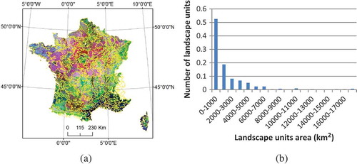
The stratification in radiometrically homogeneous landscape units (Bisquert, Bégué, and Deshayes 2015) was obtained from coarse resolution image time series (MODIS) performed with the software eCognition Developer 8.0 (Definiens 2009). First, a principal component analysis (PCA) was used for reducing the number of input images. Then, unsupervised methods (Johnson and Xie 2011; Zhang, Xiao, and Feng 2012) were used as a comparative analysis of several stratifications obtained with different input variables and different segmentation parameters. These methods allow to select the stratification that led to the highest homogeneous units being different from its neighbors. The final LUs map (Figure 1) was obtained from the combination of the enhanced vegetation index (EVI) and the second moment texture of April, July, and December (obtained as the average of the images of those months for the years 2007–2011) using the following eCognition parameters: scale factor 15 and shape 0. A total of 300 radiometrically homogeneous regions, hereafter referred to LUs, were identified with an average size of 1820 km² (3.2 km² for the smallest one, 17 500 km² for the largest one).

Figure 1. (a) MODIS-based LUs obtained by segmenting three EVI and three second moment images (scale parameter of 15 (Bisquert, Bégué, and Deshayes 2015), superimposed to a color composition of MODIS EVI of April (R), July (G), and December (B) averaged over 2007–2011. (b) Distribution of the LUs areas. For full color versions of the figures in this paper, please see the online version.

Environmental data

The typical variables used in landscape mapping are: climate, topography, parent material and land cover (Mücher et al. 2010). We used these environmental variables to analyze the LUs previously obtained by the unsupervised stratification of the MODIS images.

At the national scale, the climatic variables used in the present work are the air temperature and the precipitation. Temperature data were obtained from Meteo France website for 181 climate stations. Average annual maximum and minimum temperatures were calculated over the 2007–2011 period (same period as the one used in the stratification procedure). An interpolation was performed using the inverse distance weighted (IDW) function of ArcGis in order to obtain the temperature map over France (Figure 2(a and,b)). The precipitation map was obtained from Joly et al. (2010) by interpolation of the average annual cumulated precipitations measured in 4000 Meteo France climatic stations over the 1971–2000 period (Figure 2(c)).

Figure 2. Environmental variables used in the explanatory analysis of the stratification: (a) average maximum temperature (Météo France; 2007–2011); (b) average minimum temperature (Météo France; 2007–2011); (c) normal annual cumulated precipitations (Joly et al. 2010); (d) elevation (GTOPO 30); (e) parent material (Van Liedekerke, Jones, and Panagos 2006). Only the nine dominant parent materials of the STU are represented for the sake of clarity; (f) CORINE land cover 2006 (European Environment Agency 2007). Only the five main (level 1) categories are  shown for the sake of clarity. The LUs map obtained in Bisquert, Bégué, and Deshayes (2015) is superposed in all cases. For full color versions of the figures in this paper, please see the online version.

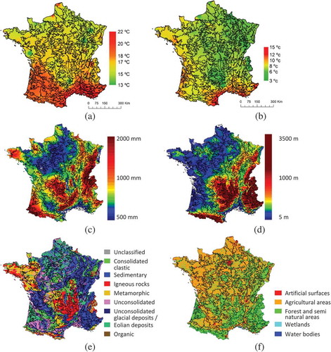
The topography was obtained from the GTOPO30 provided by the USGS (Figure 2(d)). The elevations in GTOPO30 are regularly spaced at 30-arc seconds (approximately 1 km) and the source data is the digital terrain elevation data (DTED), which is a topographic raster spaced at 3-arc seconds (approximately 90 m).

The parent material map was obtained from the European Soil Database (Van Liedekerke, Jones, and Panagos 2006). The variable used was the dominant parent material class of the soil typological unit (STU), which includes 91 types. In Figure 2(e), only the nine major classes are represented.

The land cover product used at the national level was the Corine Land Cover 2006 (CLC2006) map (European Environment Agency 2007) derived from optical decametric images (Landsat, SPOT-4 and IRS). The minimum mapping unit is 25 ha and the minimum width of linear elements is 100 m. The CLC nomenclature includes 44 land cover classes, grouped in a three-level hierarchy. In Figure 2(f), only the five main (level 1) categories are represented.

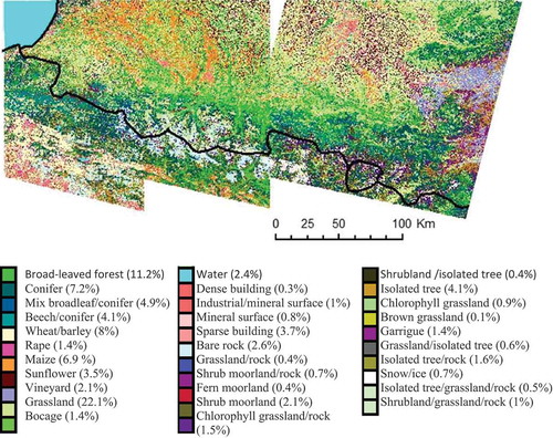
The national scale study was completed by a regional scale analysis. For this, we used a recent land cover map of the Pyrenean region. This land cover map was produced by the Centre d’Etudes Spatiales de la BIOsphère (CESBIO) from a set of Landsat images (Masse, Ducrot, and Marthon 2011) acquired over 2009 and 2010. The difficulty to obtain cloud-free images acquired at close dates over the entire region led them to use three different image data sets composed as follows:

• Land 1: 28/05/09, 29/06/09, 21/07/09.

• Land 2: 14/02/09, 18/03/09, 22/06/09

• Land 3: 20/07/10, 21/08/10, 22/09/10.

The Pyrenean land cover map obtained is composed of 32 classes (Figure 3).

Figure 3. Pyrenean land cover map (adapted from http://www.cesbio.ups-tlse.fr/newsletter_cesbio/numero8/Vmail.html#sudouest1, accessed 10/06/2013). The fraction of the class presence is given in parenthesis. The black line corresponds to the France–Spain border. For full color versions of the figures in this paper, please see the online version.

Methodology

The evaluation of the LUs identified in Bisquert, Bégué, and Deshayes (2015) in terms of landscape mapping faces two main difficulties. (1) There is no landscape map that can be used as a reference for the validation process. (2) There is no ready-to-use method to evaluate segmentation results with external data, and to analyze boundaries quality. Therefore we had to define the strategy and methods to evaluate the stratification. The global strategy consisted in (1) performing a statistical analysis of the separability of the LUs in terms of environmental variables (quantitative and qualitative variables), and (2) assessing the meaning of the boundaries between neighboring LUs defined by the segmentation procedure (hereafter referred to the boundaries firmness). This strategy, and the scale (national vs. regional) at which it is applied, is summarized in Figure 4.

Figure 4. Scheme of the analysis performed and data used.

Separability of neighboring LUs in terms of environmental variables

The first step of the analysis (Figure 4) consisted in analyzing the separability between neighboring LUs for each environmental variable (air temperature, precipitation, altitude, parent material, and land cover). The variables leading to the highest separability were chosen as the most representative for explaining the LUs. According to the type of variables used (quantitative and/or qualitative), different types of statistical analysis were performed: Moran’s index was used for quantitative variables, and Spearman’s rank correlation index for qualitative variables.

In the case of quantitative variables (climate and topography), the average values of each variable (maximum and minimum air temperatures, annual rainfall, and altitude) were obtained for each LU. Then, Moran’s Index, measuring the global autocorrelation between neighboring LUs, was calculated for each mean variable (Fotheringham, Brunsdon, and Charlton 2000).

In the case of qualitative variables (land cover and parent material), we used the Spearman’s rank correlation coefficient. This coefficient permits to calculate the correlation between the classes’ ranks of two LUs. A high correlation between two LUs means that the composition of classes in the two LUs is similar. Spearman correlation has been used in several studies for comparing classifications obtained from different methods or different years. Cherrill et al. (1995) used it to analyze the correlation between two classifications of the same area obtained in different years. Wade et al. (2003) used t-tests, Spearman rank correlation index, absolute difference and cluster analysis for studying the differences in landscape metric. It has also been used for comparing or evaluating the correlation between variables, such as landscape metrics (Styers et al. 2010; Aguiar, Fernandes, and Ferreira 2011; Liu et al. 2013), in order to reduce the redundancy of correlated variables in a study. In this study, the composition of the land cover and parent material classes was obtained for each LU. As the comparison should be settled in classes with substantial presence, only the land cover classes displaying an occupation larger than 10% in both LU were used.

The Spearman correlation r is thus obtained as shown in Equation (1):

(1)

where d_i is the difference between the ranks, and n is the number of classes.

To test the statistical significance of the Spearman correlation, the t-test was used. The t-value is obtained from Equation (2):

(2)

The degree of freedom is (n – 2). The significance is obtained comparing the t-value with the reference tables. A p-value greater than 0.05 indicates that the correlation obtained is not significant at 95% confidence level, meaning that the two neighboring LUs are not correlated in terms of the qualitative variable used.

Analysis of boundaries firmness

For the evaluation of the boundaries, an innovative procedure for analyzing the firmness of the strata boundaries in terms of land cover was developed and is presented in this section. The evaluation was performed at two different scales: the whole French territory, and the French Pyrenean region for which a more detailed land cover map was available.

Boundaries are defined as the lines separating two neighboring LUs. The goal here was to identify if the boundaries are firm or flow. If a boundary is firm, it means that the landscape characteristics are clearly different on both sides of the boundary. This analysis was performed using the Pyrenean land cover map rather than the Corine land cover map, because we expected it to be more accurate, and because the years of the map (2009–2010) agree with the delineation of the LUs (2007–2011). Therefore, this analysis was performed only at regional scale, in the French Pyrenean area.

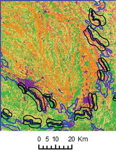
To analyze the borders quality, only areas close to the border should be analyzed. In this sense, several pairs of test areas were defined along each boundary (see example in Figure 6), one at each side of the boundary. When possible, at least three pairs of test areas were delineated for each boundary, however, in short boundaries only one or two pairs were defined. The Spearman correlation index was obtained for all the pairs in terms of the qualitative variables leading to higher separability in the previous analysis. Afterwards, according to the number of test pairs displaying a significant correlation in a boundary, we classified each boundary as firm (all the pairs showed non-significant correlation), highly firm (less than 50% of the pairs were correlated), medium firm (equal number of significant and non-significantly correlated pairs), lowly firm (more than 50%), or flow (all the pairs were correlated).

Figure 5. Simplified Pyrenean land cover map (see Table 2), overlaid with the stratification results obtained by Bisquert, Bégué, and Deshayes (2015), and divided in three zones (land 1: red; land 2: blue; land 3: pink) that correspond to different Landsat image acquisition dates. For full color versions of the figures in this paper, please see the online version.

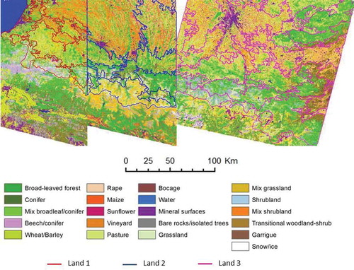
Figure 6. Example of test areas (black lines) along the boundaries (blue line) between neighboring LUs used for analyzing the boundaries quality. The legend is the same as in Figure 5. For full color versions of the figures in this paper, please see the online version.

Results

Characterization of the LUs in terms of environmental variables

The results obtained for the quantitative environmental variables at the national scale (Figure 2(a)–(d)), are shown in Table 1. A low value of the Moran’s index indicates a low correlation between neighboring LUs, i.e., a good explanatory variable in terms of separability of the units. We observed that the lowest value corresponded to the altitude (0.48), making it the most discriminant variable of the LUs, while the highest value was obtained for the maximum temperature (0.86). However, the four values were significant at 95% confident level, which indicates the existence of spatial autocorrelation, therefore none of these variables alone is capable to explain the different LUs.

Table 1. Moran’s index calculated on the environmental quantitative variables, at national scale.

	Altitude	T_max	T_min	Precipitation
Moran’s index	0.48	0.86	0.69	0.73

For the qualitative environmental variables (Figure 2(e,(f)) analysis at the national scale, the Spearman rank correlation coefficient, and its corresponding p-value were obtained for all possible pairs of neighboring LUs (620 pairs). For the land cover analysis, 92% of the correlations between neighboring LUs were not significant, we can consider that the two LUs are significantly different in terms of land cover composition. For the parent material analysis, this percentage was 93%. Thus, we could conclude that the land cover composition (Figure 2(f)) and parent material (Figure 2(e)) are good explanatory variables of the LUs.

At the regional scale, because of the differences in the dates used to obtain the land cover classification for each tile, the segmentation in LUs was divided in three zones (Figure 5). Moreover, because of the low presence of some land cover types, 17 of the original classes were merged into 6 new classes (Table 2) to simplify the analysis; the other classes (15) were not changed. The new classification in 21 classes is shown in Figure 5.

Table 2. Land cover classes correspondence between the Pyrenean cover map (Figure 3) and the simplified Pyrenean cover map (Figure 5).

New land cover	Original cover
Grassland	Chlorophyll grassland
	Brown grassland
Mix grassland	Grassland/bare rock
	Chlorophyll grassland/bare rock
	Grassland/isolated tree
	Isolated tree/grassland/bare rock
Shrubland	Fern moorland
	Shrub moorland
Mix shrubland	Shrub moorland/bare rock
	Shrubland/isolated tree
	Shrubland/grassland/bare rock
Mineral surfaces	Dense building
	Industrial/mineral surface
	Mineral surface
	Sparse buildings
Bare rocks/isolated trees	Bare rock
	Isolated tree

Note: The classes that are common to both maps are not presented in the table.

At regional scale, we tested a total of 56 pairs of neighboring LUs and only one pair (2 %) showed a significant correlation between both neighboring LUs (p-value <0.05) in terms of land cover.

These results obtained at national and regional scales, showed that the LUs map based on MODIS images (Bisquert, Bégué, and Deshayes 2015) led to LUs, which are different from its neighbors in terms of land cover and parent material composition.

Analysis of boundaries firmness

For the analysis of the boundaries quality, test areas were identified on both sides of each neighboring LUs boundary as shown in Figure 6. A total of 56 pairs of neighboring LUs (Figure 5) including 161 pairs of test areas were analyzed. Spearman’s correlation index was calculated for each pair of test areas in terms of the qualitative environmental variables (parent material and land cover).

When considering the land cover, 89% of the pairs of test areas did not present a significant correlation; this means that a large majority of the test areas across the boundaries had a different land cover composition, and therefore, that the boundaries were well defined and meaningful in terms of land cover. The percentage of non-correlated pairs when using parent material was lower (53%), meaning that the parent material is not a good explanatory variable of the boundaries. We could then conclude that the limits of the boundaries are well explained by land cover.

Based on these results, the boundaries firmness was thus analyzed only in terms of land cover. The percentage of test areas delineated in each boundary presenting a significant correlation was used for defining the boundaries firmness. The analysis in terms of land cover showed that there were 43 (out of 56) boundaries that could be considered as firm, 7 boundaries which were highly firm, 3 as medium firm and 1 flow.

Discussion

Landscape mapping based on remote-sensing images benefits from the spatial and temporal continuity of the satellite data. Remote sensing is often the only way to make spatiotemporal analysis of landscapes, and gives the opportunity of looking back into the past thanks to the high volume of archive images (Groom et al. 2006).

An objective methodology for delineating homogeneous regions in the French territory was obtained from time series of coarse resolution satellite images in Bisquert, Bégué, and Deshayes (2015). This stratification was considered as a LUs map, and there was a need for a qualitative evaluation of this map using external data. To conduct this evaluation, we faced two difficulties: (i) there was no landscape map of the French territory to be used for validation; (ii) there was no ready-to-use method to objectively evaluate segmentation results with external data and no method to analyze boundaries quality.

In this paper, we developed and presented original solutions to evaluate MODIS satellite-based LUs map, using environmental and land cover data. The first solution consisted in identifying the environmental variables that distinguished the LUs from their neighbors, and the second one consisted in analyzing the meaning and quality of the boundaries between neighboring LUs. High autocorrelation (significant at the p < 0.05 level) of climatic variables was found in the neighboring LUs, which was not surprising because the LUs sizes are relatively small and in the French territory there are not high gradients in climate variables. We would expect climate variables to be significant in segmentation results leading to larger units (e.g. climatic zones). Topography presents higher gradients but not enough for being representative of the relatively small LUs, we would still expect being more representative of larger units. Contrary, land cover and parent material were good explanatory variables of the LUs based on the Spearman rank index obtained under the assumption that only the classes occupying more than 10% of each LU should contribute to the analysis. This result suggested that the use of vegetation and texture indices time series captures the essence of vegetation phenology and land cover, even at the 250 m spatial resolution of MODIS.

In this paper, we tried to go further in the segmentation evaluation by explaining and quantitatively evaluating the segments boundaries. The evaluation of boundaries was a major challenge because we did not find any study analyzing the segmentation boundaries with external data. Geometrical evaluation can be done with reference data (Whiteside, Maier, and Boggs 2014). However, when no reference data exists, the boundaries analysis is usually performed by an expert. This evaluation is not quantifiable, and is especially difficult to perform when using coarse resolution images. Therefore, we developed a method for assessing boundaries quality based on Spearman rank’s correlation. This innovative procedure could serve to evaluate the boundaries between neighboring segments in other object-based stratifications. This analysis showed that the land cover was the best explanatory variable for the boundaries, with 89% of the test areas being not correlated.

The main limitation that can be found when applying the procedures presented in this paper is the need of quality input data to be used for the evaluation of the LUs that may not be available everywhere.

We showed in this paper the existing link between the LUs obtained from MODIS data alone, and the environmental variables. This LUs map, as it is, is useful for applications that need a stratification of the territory, such as land cover classifications at local scale (Cano et al. 2014). The next step will be to label the LUs and classify them in terms of the environmental variables in order to obtain finally a landscape map of the French territory.

Conclusion

OBIA had been previously used for delineating homogeneous regions from time series of MODIS images. These regions were obtained with an unsupervised analysis of the input variables and segmentation parameters and were considered as LUs. In this paper, we showed the link that exists between the environmental variables and the LUs delineated from remote-sensing data. To do this, we developed a procedure that allowed to evaluate the segmentation results in terms of external environmental data, and also to evaluate the quality of the segments boundaries. An analysis of the stratification results at national scale showed that the best explanatory variables of the LUs are land cover and parent material. The boundaries analysis performed at regional scale showed that the boundaries between neighboring LUs are well explained by land cover. These results confirm the hypothesis made in Bisquert, Bégué, and Deshayes (2015) that time series of coarse resolution remote-sensing images can capture landscape identities even if individual land cover classes cannot be identified on the image. Moreover, the procedures developed here are a useful tool for objectively evaluating segmentation results and thematic maps using external data and could be applied to different types of segmentation results and using different variables.

Acknowledgements

This work was supported by IRSTEA funds (post-doctoral contract) and the financial support of The French Ministry of Agriculture, project TelIAE “Télédétection des infrastructures agro-écologiques” coordinated by CETIOM, The Technical Centre for Oilseed Crops and Industrial Hemp. The authors would like to thank MeteoFrance, Daniel Joly, the US Geological Service, the European Commission, the European Soil Bureau Network, the European Environment Agency and CESBIO for providing the environmental data (meteorological data, elevation, parent material, and land cover) used in this work.

Disclosure statement

No potential conflict of interest was reported by the authors.

Additional information

Funding

This work was supported by IRSTEA funds (Mar Bisquert post-doctoral contract) and the financial support of The French Ministry of Agriculture, project TelIAE “Télédétection des infrastructures agro-écologiques” coordinated by CETIOM, The Technical Centre for Oilseed Crops and Industrial Hemp.

References

- Aguiar, F. C., M. R. Fernandes, and M. T. Ferreira. 2011. “Riparian Vegetation Metrics as Tools for Guiding Ecological Restoration in Riverscapes.” Knowledge and Management of Aquatic Ecosystems 402: 21. doi:10.1051/kmae/2011074.
- Bisquert, M., A. Bégué, and M. Deshayes. 2015. “Object-Based Delineation of Homogeneous Landscape Units at Regional Scale Based on MODIS Time Series.” International Journal of Applied Earth Observation and Geoinformation 37: 72–82. doi:10.1016/j.jag.2014.10.004.
- Cano, E., M. Bisquert, J. P. Denux, and V. Chéret. 2014. Contribution of an Object-Oriented Image Segmentation to Forest Cover Mapping. Presented at Global Vegetation Monitoring and Modeling, Avignon, FRA (2014-02-03 - 2014-02-07) Avignon.
- Cherrill, A. J., C. McClean, P. Watson, K. Tucker, S. P. Rushton, and R. Sanderson. 1995. “Predicting the Distributions of Plant Species at the Regional Scale: A Hierarchical Matrix Model.” Landscape Ecology 10 (4): 197–207. doi:10.1007/BF00129254.
- Definiens. 2009. Ecognition Developer 8.0 User Guide. Munich, Germany: Definiens AG.
- Dronova, I., Peng Gong, Nicholas E. Clinton, Lin Wang, Wei Fu, Shuhua Qi, and Ying Liu. 2012. “Landscape Analysis of Wetland Plant Functional Types: The Effects of Image Segmentation Scale, Vegetation Classes and Classification Methods.” Remote Sensing of Environment 127: 357–369. doi:10.1016/j.rse.2012.09.018.
- European Environment Agency. 2007. CLC2006 Technical Guidelines, 17. http://www.eea.europa.eu/publications/technical_report_2007_17.
- European Environment Agency. 1995. Europe’s Environment. The Dobris Assessment. David Stanners And Philippe Bourdeau. Copenhagen. http://www.eea.europa.eu/publications/92-826-5409-5
- Foody, G. M. 2002. “Status of Land Cover Classification Accuracy Assessment.” Remote Sensing of Environment 80 (1): 185–201. doi:10.1016/S0034-4257(01)00295-4.
- Fotheringham, A. S., C. Brunsdon, and M. Charlton. 2000. Quantitative Geography: Perspectives on Spatial Analysis. London: Sage.
- Groom, G., C. A. Mücher, M. Ihse, and T. Wrbka. 2006. “Remote Sensing in Landscape Ecology: Experiences and Perspectives in a European Context.” Landscape Ecology 21 (3): 391–408. doi:10.1007/s10980-004-4212-1.
- Guitet, S., J.-F. Cornu, O. Brunaux, J. Betbeder, J.-M. Carozza, and C. Richard-Hansen. 2013. “Landform and Landscape Mapping, French Guiana (South America).” Journal of Maps 9 (3): 325–335. doi:10.1080/17445647.2013.785371.
- Hazeu, G. W., M. J. Metzger, C. A. Mücher, M. Perez-Soba, C. Renetzeder, and E. Andersen. 2011. “European Environmental Stratifications and Typologies: An Overview.” Scaling Methods in Integrated Assessment of Agricultural Systems 142 (1–2): 29–39. doi:10.1016/j.agee.2010.01.009.
- Ismail, K., V. A. I. Huvenne, and D. G. Masson. 2015. “Objective Automated Classification Technique for Marine Landscape Mapping in Submarine Canyons.” Marine Geology 362 (April): 17–32. doi:10.1016/j.margeo.2015.01.006.
- Johnson, B., and Z. Xie. 2011. “Unsupervised Image Segmentation Evaluation and Refinement Using a Multi-Scale Approach.” ISPRS Journal of Photogrammetry and Remote Sensing 66 (4): 473–483. doi:10.1016/j.isprsjprs.2011.02.006.
- Joly, D., T. Brossard, H. Cardot, J. Cavailhes, M. Hilal, and P. Wavresky. 2010. “Les Types de Climats En France, Une Construction Spatiale.” Cybergeo. doi:10.4000/cybergeo.23155.
- Liu, D., S. Hao, X. Liu, B. Li, S. He, and D. N. Warrington. 2013. “Effects of Land Use Classification on Landscape Metrics Based on Remote Sensing and GIS.” Environmental Earth Sciences 68 (8): 2229–2237. doi:10.1007/s12665-012-1905-7.
- Masse, A., D. Ducrot, and P. Marthon. 2011. “Tools for Multitemporal Analysis and Classification of Multisource Satellite Imagery.” Analysis of Multi-Temporal Remote Sensing Images (Multi-Temp), 2011 6th International Workshop on the, 209–212. http://ieeexplore.ieee.org/xpls/abs_all.jsp?arnumber=6005085.
- Mücher, C. A., J. A. Klijn, D. M. Wascher, and J. H. J. Schaminée 2010. “A New European Landscape Classification (LANMAP): A Transparent, Flexible and User-Oriented Methodology to Distinguish Landscapes.” Landscape Assessment for Sustainable Planning 10 (1): 87–103. doi:10.1016/j.ecolind.2009.03.018.
- Pesch, R., G. Schmidt, W. Schroeder, and I. Weustermann. 2011. “Application of CART in Ecological Landscape Mapping: Two Case Studies.” Ecological Indicators 11 (1): 115–122. doi:10.1016/j.ecolind.2009.07.003.
- Shrestha, S., and K. E. Medley. 2016. “Landscape Mapping: Gaining ‘Sense of Place’ for Conservation in the Manaslu Conservation Area, Nepal.” Journal of Ethnobiology 36 (2): 326–347. doi:10.2993/0278-0771-36.2.326.
- Smiraglia, D., G. Capotorti, D. Guida, B. Mollo, V. Siervo, and C. Blasi. 2013. “Land Units Map of Italy.” Journal of Maps 9 (2): 239–244. doi:10.1080/17445647.2013.771290.
- Styers, D. M., A. H. Chappelka, L. J. Marzen, and G. L. Somers. 2010. “Developing a Land-Cover Classification to Select Indicators of Forest Ecosystem Health in a Rapidly Urbanizing Landscape.” Landscape and Urban Planning 94 (3–4): 158–165. doi:10.1016/j.landurbplan.2009.09.006.
- Van Liedekerke, M., A. Jones, and P. Panagos. 2006. “ESDBv2 Raster Library-a Set of Rasters Derived from the European Soil Database Distribution v2. 0.” European Commission and the European Soil Bureau Network, CDROM, EUR, 19945.
- Vieira, M. A., A. R. Formaggio, C. D. Rennó, C. Atzberger, D. A. Aguiar, and M. P. Mello. 2012. “Object Based Image Analysis and Data Mining Applied to a Remotely Sensed Landsat Time-Series to Map Sugarcane over Large Areas.” Remote Sensing of Environment 123: 553–562. doi:10.1016/j.rse.2012.04.011.
- Wade, T. G., J. D. Wickham, M. S. Nash, A. C. Neale, K. H. Riitters, and K. B. Jones. 2003. “A Comparison of Vector and Raster GIS Methods for Calculating Landscape Metrics Used in Environmental Assessments.” Photogrammetric Engineering & Remote Sensing 69 (12): 1399–1405. doi:10.14358/PERS.69.12.1399.
- Whiteside, T. G., S. W. Maier, and G. S. Boggs. 2014. “Area-Based and Location-Based Validation of Classified Image Objects.” International Journal of Applied Earth Observation and Geoinformation 28: 117–130. doi:10.1016/j.jag.2013.11.009.
- Zhan, Q., M. Molenaar, K. Tempfli, and W. Shi. 2005. “Quality Assessment for Geo‐spatial Objects Derived from Remotely Sensed Data.” International Journal of Remote Sensing 26 (14): 2953–2974. doi:10.1080/01431160500057764.
- Zhang, X., P. Xiao, and X. Feng. 2012. “An Unsupervised Evaluation Method for Remotely Sensed Imagery Segmentation.” IEEE Geoscience and Remote Sensing Letters 9 (2): 156–160. doi:10.1109/LGRS.2011.2163056.