Integrating the multi-label land-use concept and cellular automata with the artificial neural network-based Land Transformation Model: an integrated ML-CA-LTM modeling framework

Abstract

Cellular automata (CA) and artificial neural networks (ANNs) have been used by researchers over the last three decades to simulate land-use change (LUC). While conventional CA and ANN models assign a cell to only one land-use class, in reality, a cell may belong to several land-use classes simultaneously. The recently developed multi-label (ML) concept overcomes this limitation in land change science. Although the ML concept is a new paradigm with nonexclusive classes and has shown considerable merit in several applications, few studies in land change science have applied it. In addition, determining transition rules in conventional CA is difficult when the number of drivers is large. Since CA has been shown as a potential model to consider neighborhood effects and ANN has been shown effective in determining CA transition rules, we integrated both CA with an ANN model to overcome limitations of each tool. In this study, we specifically extended the ANN-based Land Transformation Model (LTM) with both a CA-based model and the ML concept to create an integrated ML-CA-LTM modeling framework. We also compared, using standard evaluation measures, differences between the proposed integrated model with a conventional CA-based LTM model (called the ml-CA-LTM). Parameterization was made using a learning and testing procedure common in machine learning. Results showed that the modified LUC model, ML-CA-LTM, produced consistently better goodness of fit calibration values compared to the ml-CA-LTM. The outcome of this modified model can be used by managers and decision makers for improved urban planning.

Keywords:

• artificial neural networks
• cellular automata
• land-use change
• mono-label class
• multi-label classes

View correction statement:

Erratum

Introduction

Land change is known for being a complex process across spatial and temporal scales (Brown et al. 2013). Land change scholars usually combine various endogenous factors (e.g., neighborhood effect and interaction among factors as well as land-use classes) and exogenous factors (e.g., slope and transport systems, human behavior, socioeconomic and cultural factors) across multiple scales (Lambin and Geist 2006) to explain this complexity. Scientists from various disciplines such as computer science, geography, cartography, and environmental engineering, have contributed to land change science (cf. Turner, Lambin, and Reenberg 2007; Mustard et al. 2004; Rindfuss et al. 2004; Lambin et al. 2001; Azari et al. 2016). Machine learning techniques (Witten and Frank 2005), due to their ability to fit nonlinear functions, have been used to learn about land-use change (LUC) patterns (e.g., Pijanowski et al. 2002a, 2006). Machine learning techniques include various approaches such as artificial neural networks (ANNs) (Li and Yeh 2002; Basse et al. 2014), support vector machines (Yang, Li, and Shi 2008; Huang, Xie, and Tay 2010), genetic algorithms (Shan, Alkheder, and Wang 2008), classification and regression trees (Tayyebi and Pijanowski 2014), multivariate adaptive regression splines (Tayyebi et al. 2014b), among others (Bagan and Yamagata 2015; Omrani et al. 2015a, 2015b).

The Land Transformation Model (LTM), which is an ANN-based model, is one of the well-known machine learning tools that has been used and applied to various places across the globe, including Asia (Pijanowski et al. 2009), Europe (Pijanowski, Alexandridis, and Mueller 2006), Africa (Tayyebi et al. 2014b), and the United States (Pijanowski et al. 2002b; Tayyebi et al. 2013; Pijanowski et al. 2014). After over a decade of development and assessment, the LTM has been used to: (1) determine the level of uncertainty in land change model output and land change contexts (Pijanowski et al. 2014; Ray et al. 2012); (2) couple to other process-based models to understand how LUC alters ecosystem dynamics (Pijanowski et al. 2007; Wayland et al. 2003); and (3) be used as baseline data layer for online decision support tools (Ray et al. 2012). The LTM has also been used in conjunction with participatory and role playing games so that the complexity of LUC can be understood using a combination of computer-based and human-based decision-making (e.g., Washington-Ottombre et al. 2010; Olson et al. 2008). Finally, the model has been configured to run “backward” in order to create historical land-use maps (Pijanowski et al. 2007) with the aim of understanding how legacies of land use affect current ecosystem processes.

In previous studies, either the application of a single LUC (e.g., Pijanowski et al. 2002b) or multiple LUCs (Pijanowski et al. 2014) have yielded somewhat satisfactory performing models using single-class assignments of spatial units. The original version of the LTM (Pijanowski et al. 2002a) has been designed to simulate conditions of change and persistence. Many of these parameterizations (e.g., Tayyebi, Perry, and Tayyebi 2014a) performed relatively well during calibration steps. For example, Tayyebi et al. (2014b) used the LTM to simulate urbanization, forest growth, and agriculture gain as independent routines, comparing and contrasting model performance in both the United States and East Africa. They found that ability of the LTM to predict change for each class varied by land-use class, as well as location. Yet, another configuration of the model, designed to simulate multiple LUCs simultaneously (Pijanowski et al. 2014), was also shown to deal with more than two land-use classes at a time. However, even the LTM, with multiple LUCs’ capabilities, makes the assumption that each cell belongs only to one land-use class at each time. Finally, the LTM, configured as a hybrid model, has been coupled with spatially explicit models such as cellular automata (CA) to make calibration run (e.g., finding the transition rules of CA model) faster (Li and Yeh 2002; Basse et al. 2014). For example, Li and Yeh (2001) integrated CA with ANN to calibrate a CA-ANN model to determine transition rules for urbanization and land-use management.

With CA models, areas are presented by a grid of cells and interaction among these cells defines the global behavior of land-use systems. According to literature (Clarke, Hoppen, and Gaydos 1997; Couclelis 2005; Wolfram 1994, 2002; Akın, Clarke, and Berberoglu 2014), CA can simulate complex LUC systems (in sensu Lambin et al. 2001). In the early 1990s, the use of CA models became more common as a tool to study land-use dynamics. In fact, CA models were accepted as one of the most well-known tools for better understanding the hidden patterns in land-use data (White, Uljee, and Engelen 2012; Blecic, Cecchini, and Trunfio 2013). The interest in using CA for modeling LUCs was triggered by the fact that CA models are spatially explicit, and have many common characteristics with the land-use system.

The previous studies of LUC modeling (e.g., both ANN and CA) were limited with using the multi-label (ML) concept. Thus, it is required to develop a LUC model that can simulate mixed land-use classes. Omrani et al. (2015a) have recently showed the merit of the ML concept in LUC modeling. These researchers utilized the ML k-nearest neighbors (MLkNN) technique, but did so outside the CA framework. The current paper takes the next step by introducing the new concept of ML into an integrated CA–LTM model. ML is important to LUC modeling in several ways. First, many places have mixed land uses and this needs to be represented in models. For example, farm fields may also be used as wind farms and places for grazing of animals during pasture rotations. Second, in areas where there is a lot of land-use fragmentation, some pixels are not large enough to represent one homogenous patch of a land use; they might have more than one. This is especially true for areas along the urban–rural fringe where complex shorelines create boundaries of land and water where high spatial detail is needed. Third, many “snapshots” of land use/cover across large areas contain locations in transition. Former forest or agricultural lands could be bare soil in a satellite image or aerial photo as land is being prepared for development. These cells could be considered a hybrid use at that moment in time. Finally, assigning multiple tags to a cell means that more information can be associated with a location, such as levels of “intensity.”

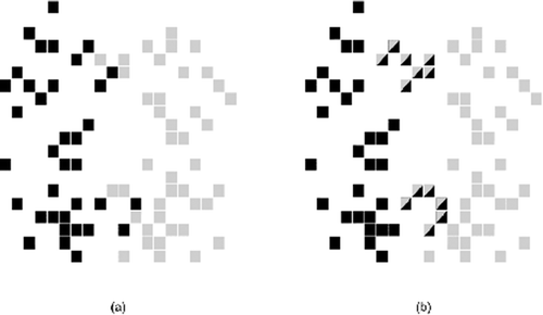
The ML classification is different from the mono-label (ml) classification approach (Figure 1(a)–(b)). An ML cell can have more than one class at the same time. However, an ml cell can only have one elementary class (i.e., single label). Moreover, the ML classification is different from fuzzy logic (Boutell et al. 2004). Fuzzy logic addresses the ambiguity in the border of multiple land-use classes (e.g., 0.2 for forest, 0.3 for agriculture, and 0.5 for urban; Malczewski 2006). Fuzzy logic employs a nondiscrete membership function to characterize ambiguity and uses defuzzification to derive a crisp land-use class (Power, Simms, and White 2001). In contrast, ML classification is able to assign multiple land uses to one cell (Sorower 2010). The content for different land-use classes is distinct (e.g., urban, agriculture, and forest). In addition, the sum of fuzzy functions usually is normalized to 1, while no such constraints apply to the ML classification.

Figure 1. (a) mono-label classification (ml) with two land-use classes (gray and black) and (b) Multi-Label classification (ML) with cells belonging to both classes (squares split by the two colors).

Most of the previous applications of LTM (binary and multi-class) as well as CA models correspond to a ml land-use concept. This sort of LUC modeling is not realistic due to the fact that one cell in reality might belong to multiple land-use classes. According to White, Uljee, and Engelen (2012), most LUC models have a major drawback which is the discrete state assignment for cells – a cell has a one state at a time – which is unrealistic for areas with mixed land uses. Though there is progress in LUC modeling, the elaboration of an appropriate LUC model that can simulate mixed LUCs is challenging (Couclelis 2005; Batty 2011). To overcome the existing gap in literature, a potential solution is the concept of ML instead of ml. In this study, we integrated the LTM with CA and the ML concept to simulated mixed LUCs (called the ML-CA-LTM). An ANN algorithm with the Backpropagation Multi-Label Learning (BP-MLL) is used to determine CA transition rules (Zhang and Zhou 2006).

We applied the developed model on rich datasets from the country of Luxembourg, Europe, to study mixed LUCs. We validated the model using the common goodness-of-fit measurements for ML learning including accuracy, precision, and an F-measure. We also compared the proposed model with the conventional LTM model (called hereafter the ml-CA-LTM), based on a set of measures carefully selected to demonstrate the added value of the new model. ML-CA-LTM offers to the wider community of researchers working on land-use modeling, a new research framework that addresses the current shortcomings of the conventional LTM and CA models when dealing with mixed land use (i.e., ML class).

Methods and materials

Multi-label cellular automata-Land Transformation Model: ML-CA-LTM

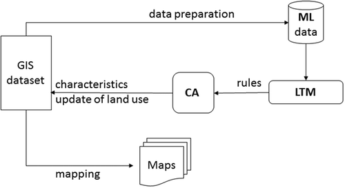
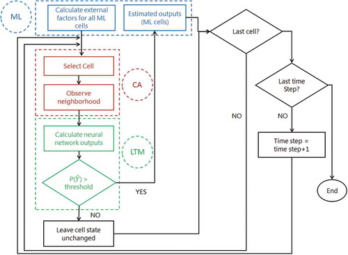
The new model has three integrated components (ML, CA, and LTM). Figure 2 shows the entire process of integrating the ML land-use concept and CA with the ANN-based LTM (ML-CA-LTM).

Figure 2. Conceptual diagram of the ML-CA-LTM model.

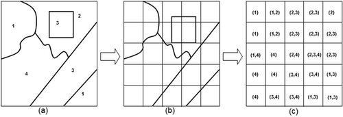
(1) ML: The preprocessing consists of converting the vector map to raster using a soft classification procedure that lets a cell have more than one land-use class. As a result, a cell may be associated with several labels (see Figure 3), for instance, when it is on the border of residential and industrial areas. The procedure of soft classification/rasterization is different than the hard classification (using a dominant class) which is extensively applied in LUC science.

Figure 3. Conversion of a vector map to a raster map with ML: (a) vector data containing polygons with land-use codes; (b) rasterizing vector data; (c) the value of each grid in raster space depends on the land-use code of the polygons which cover them.

(2) CA: The new model has all the characteristics of a CA model but with a new extension mainly related to a cell’s state and its transition rule: (a) Cell: It has a regular rectangular form with 1 ha resolution. In general, the shape of cells in CA can be regular or irregular; (b) Time: The status of each cell varies across time steps; (c) Extent: It corresponds to the entire study area; (d) State: Each cell has a unique state at each time from a finite set of states. Each cell may have several states (classes/labels) at the same time; (e) Neighborhood: It defines the interaction among cells. The neighborhood relation is local and uniform (e.g., Moore neighborhood). The number of cells in this neighborhood and correspondence to each class is computed and considered as an input variable in the model; and (f) Transition rule: It determines the future state of each cell using a set of explanatory variables, the current state of the cell, and the states of the cells in the local neighborhood.

(3) LTM: LTM, which is an ANN-based LUC model, uses geographic information system (GIS) layers to simulate LUCs (Pijanowski et al. 2014). ANNs build a functional relationship by passing information from inputs through a network of nodes that have activation and bias function coefficients that approximate the pattern of the LUCs coded as outputs; as such, the simulation mimics the behavior of neurons and learning by a vertebrate brain (Reed and Marks 1998; Li and Yeh 2002; Grekousis, Manetos, and Photis 2013; Mas et al. 2004; Basse et al. 2014).

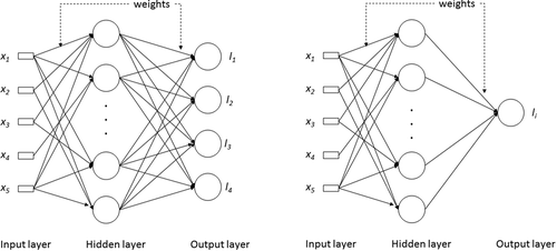
For integrating the ML concept with LTM, the Backpropagation algorithm for ML learning (BP-MLL) has been used (Zhang and Zhou 2006). The BP-MLL employs a multilayer perceptron with three consequent layers called input, hidden, and output layers to learn the spatial and temporal LUC patterns (Figure 4). The hidden layer in BP-MLL is able to detect nonlinear patterns in land-use data (Heaton 2005). To address the dependence among labels/classes in BP-MLL, the error function is modified to better understand the spatial and temporal patterns of ML learning. The minimization of the error function is performed using a gradient descent technique called mean square error (Zhang and Zhou 2006). The number of nodes in the hidden layer is important because it impacts the model’s performance (Pijanowski et al. 2014). Pijanowski et al. (2002a) built an ANN where the number of hidden nodes was equal to the number of input nodes. In the current paper, the number of hidden nodes is fixed by adjusting the error rate for several numbers of hidden nodes and the optimal number corresponds to the minimum value of the error rate, as stated by Omrani et al. (2013).

Figure 4. Architectures of the neural network BP-MLL (in the left) and BP (in the right) showing input, hidden and output layers.

ML-CA-LTM versus ML-CA-LTM

There are generally two ways to apply an ML classification (Yang et al. 2012): (1) transformation and (2) adaptation. The transformation methods consist of converting the ML classification task to a series of binary tasks which then applies an ml classifier to each one (case of the ml-CA-LTM). However, the adaptation methods handle the ML data without any transformation and then apply an ML classifier (case of the ML-CA-LTM).

The ml-CA-LTM and ML-CA-LTM use ANN to calibrate the CA-based land-use model. The ml-CA-LTM and ML-CA-LTM models use ANN with BP (Backpropagation for ml learning approach with one output label at a time) and BP-MLL (Backpropagation adapted for ML learning with four output labels simultaneously), respectively (see Figure 4; Tayyebi and Pijanowski 2014). The BP algorithm uses the mean square error and the BP-MLL uses a modified error function to address the dependence among labels (Zhang and Zhou 2006).

We present, hereafter, the main processing steps of the BP-MLL neural network algorithm used in the ML-CA-LTM model (Figure 5). These steps can very well be applied to the ml-CA-LTM as well. However, the BP-MLL learning algorithm simulates complexity that BP cannot. These steps include: (1) Assigning random weights; (2) For a given set of inputs, a set of known outputs or observed outputs are assigned (using a binary coding, e.g., the ML class (1,1,1,0) indicates that the first three elementary labels are present in the cell); (3) The network then calculates the outputs using the assigned random weights; (4) The ANN then compares the outputs that the network calculated (estimated outputs) with the observed outputs; (5) The difference between estimated and observed outputs is calculated using an error function; (6) The ANN then updates the weights using the BP-MLL algorithm to minimize the error; and (7) Once the weights are updated, the neural networks calculate the estimated outputs from the obtained set of probabilities using an optimal threshold. The repetitive learning process usually ends when the model reaches an acceptable error rate or maximum number of iterations set by the user.

Figure 5. Processing steps of the ML-CA-LTM model. Note that the estimated label set for a given cell is fixed by a threshold which is to be optimized, as suggested by Zhang and Zhou (2006).

Model calibration and evaluation

The stratified random sampling approach was used to divide the entire data into learning and testing subsets within each land-use class (stratum). We fit the model to the learning set and assessed the evaluation measures (metrics) to the testing set. We replicated this process of partitioning, fitting the model, and evaluating the metrics N times, obtaining N sets of the metrics. Their average is the overall evaluation measure. We use this method throughout the set of simulations. Using spatial data in t1, we generate a set of variables that we assume can explain ML LUCs as model inputs. The model output is mixed LUCs between t1 and t2. Based on the training dataset, the learning algorithm (i.e., BP-MLL) can capture the pattern of the land use at t2 as a function of the variables set extracted at period t1. As a result, it will be possible to simulate the land use at t3 based upon the detected pattern from the training run. The ML-CA-LTM method has two parameters, the number of neighbors used in the neighborhood configuration, k, and the number of units in the hidden layers, h.

Evaluation of the ML learning algorithm is more challenging than ml learning as the prediction for a cell obtained by ML may be correct either completely to some extent or certainly not at all (see Boutell et al. (2004) for more details). Y_i is the set of the actual labels of a spatial unit (cell x_i) and Ŷ_i = C(x_i) is the set of estimated labels for cell x_i. Our metrics depend on the following four counts: A_i = |Yi∩Ŷ_i|, the number of labels that the actual and estimated classifications have in common; B_i = |YiUŶ_i|, the number of labels that appear in at least one of the two classifications; C_i = |Ŷ_i|, and D_i = |Y_i|, the numbers of labels in the actual and estimated classifications. The metrics called accuracy (Acc), precision (Prec), recall (Rec), and F1 are defined as:

(1)

where m is the number of cells used in the testing run. F1 is the harmonic average of Prec and Rec (Omrani et al. 2015a). Like Acc, it is a symmetric function of the actual and estimated labels.

The Hamming loss (Hamm.loss) is the symmetric difference between observed and estimated labels, Y_i and Ŷ_i. This metric counts the errors of two kinds, incorrect inclusion and incorrect omission of a label. It is defined as:

(2)

where Δ shows the symmetric difference between Y_i and Ŷ_i, while Q shows the number of labels.

All five metrics are averages of fractions, and their value ranges vary between 0 and 1. Larger values of Acc, Prec, Rec, and F1 correspond to better performance, while smaller values for Hamming loss correspond to better performance.

We illustrate hereafter the evaluation measures (i.e., metrics). We use a testing set with five cells that belong to label set Y = {l₁, l₂, l₃, l₄}. Every cell can have one or several labels (observed outputs). In Table 1, we give the estimated outcomes for the given cells to show how to compute the evaluation measures.

Table 1. Example of a testing set.

Observed	Observed Class				Neural output				Estimated class				Estimated
Label set	y1	y2	y3	y4	y1	y2	y3	y4	y1	y2	y3	y4	Label set
{y1, y4}	1	0	0	1	0.5	0.1	0.6	0.2	1	0	1	0	{y1, y3}
{y2, y3}	0	1	1	0	0.3	0.7	0.4	0.1	0	1	1	0	{y2, y3}
{y1, y4}	1	0	0	1	0.5	0.2	0.2	0.6	1	0	0	1	{y1, y4}
{y2}	0	1	0	0	0.2	0.8	0.1	0.6	0	1	0	1	{y2, y4}
{y1, y3}	1	0	1	0	0.9	0.3	0.2	0.1	1	0	0	0	{y1}

Note: The selected outputs, based on an optimized threshold = 0.45, are shown in bold.

We illustrate here how the various metrics are computed, according to the definition of each metric described above:

(3)

All the presented measures (i.e., accuracy, precision, recall, hamming loss) are applied in the application section.

Implementation of ML-CA-LTM

Study area

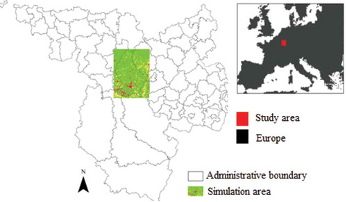
Luxembourg has attracted a lot of immigrants across entire Europe due to the socioeconomic development of its citizens. This is also due to the industrial sectors that have had a significant impact on the economic and financial status of the country, which has been ongoing since the 1970s. Despite its specific spatial constraint in term of surfaces (2586 km²) and population (512,353 inhabitants), this “small country” benefits from the strategic central geographic location within the European Union (Figure 6). Surrounded by Germany, France, and Belgium, Luxembourg attracts a variety of qualified workers with a broad array of skills to sustain its economic vitality, resulting in high-end residential communities with considerable daily mobility within Luxembourg and across border land territories.

Figure 6. Luxembourg and its bordering areas.

Land-use data

We used the biophysical land-use data as land-cover data source. There are two vector maps that represent land cover for the years 1999 and 2007 (Maps 1999, 2007). Every vector map comprises 76 land-cover classes within 6 main categories, namely: artificial, agriculture, wetlands, forest, water, and seminatural areas. In the current study, we reclassified the 76 into 4 land-cover classes: urban, industry, agriculture, and forest and did not allow changes to water and wetlands and so were not considered in our modeling framework. The reclassification was achieved with the help of local experts experienced with the biophysical dataset. Descriptions for each land-use class are:

• Urban: a variety of urban land uses, from compact urban areas to rural areas, parks, and car parking areas;

• Industrial: commercial, military, and industrial areas;

• Agricultural: all types of agricultural land, including orchards and grazing land;

• Forestry: forested land, including areas covered by shrubs, bushes, forests, and rocky areas;

In the dataset, we have the following elementary labels (i.e., classes of land use): urban, industrial, agriculture, and forest. We define a ML classification for each cell in a given year, by an element of the set {0,1}⁴, indicating for each elementary label (called ml) whether it is present in the cell or not. For example, the ML class (1,1,1,1) indicates that all four elementary labels are present in the cell. We construct the dataset with ML classes and use it for classifying land use in Luxembourg (Omrani et al. 2015a). In a vector map, features are represented by points, lines, and polygons. In the current application, we rasterize the vector map of Luxembourg (i.e., convert the vector information into a raster format) using a rectangle grid with a resolution of 100 m (cell size of 1 ha). This resolution is commonly used at a regional or national scale (White and Engelen 2000). Such resolution is appropriate to capture variability that can be partly lost at finer resolutions (Hijmans et al. 2005). We implemented the ML data preparation algorithm using GIS software and the Python programming language (see Omrani et al. 2015a for more details).

Data processing for inputs and outputs

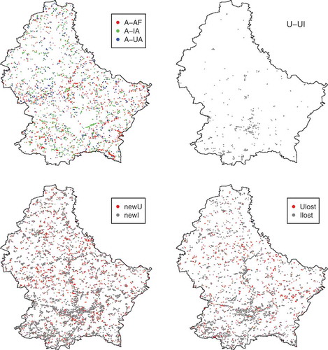
The input data are coming from various data sources including aerial photographs at two time periods 1999 and 2007, and a digital elevation model (derived from SRTM data) to illustrate the physical constraint of the studied area. The slope was derived from the digital elevation model database (Farr et al. 2007). The explanatory variables used in this study are: the state of each cell, distance to transport system (bus stations, train stations, road, and access to highway), distance to Luxembourg border area, slope, and number of each land-use class in the Moore neighborhood (Table 2). The time step was set to 8 years (due to observed time periods), which means that each iteration represents 8 years of change in the real world. Table 3 shows the land-use statistics between two time periods (1999 and 2007). Figure 7 illustrates the LUC and their spatial locations between 1999 and 2007.

Table 2. Driving features as input of the model.

Category	Variable	Description
Physical	State_cell Y = (y1,y2,y3,y4)	Multi-label class
	X1: Slope	Slope value of cell (%)
	X2: Urban_neighbours	Amount of urban cells in the 3 × 3 Moore neighborhood
	X3: Industrial_neighbours	Amount of industrial cells in the 3 × 3 Moore neighborhood
	X4: Agriculture_neighbours	Amount of agriculture cells in the 3 × 3 Moore neighborhood
	X5: Forest_neighbours	Amount of forest cells in the 3 × 3 Moore neighborhood
	X6: Water_neighbours	Amount of water cells in the 3 × 3 Moore neighborhood
City/country distances	X7: Distance_border	Distance from cell to the border of Luxembourg country (m)
	X8: Distance_main_city1	Distance from cell to the city of Luxembourg (m)
	X9: Distance_ main_city2	Distance from cell to the city of Esch (m)
	X10: Distance_ main_city3	Distance from cell to the city of Differdange (m)
Transportation	X11: Transport_neighbours	Amount of transport cells in the 3 × 3 Moore neighborhood
	X12: Distance_bus_stations	Distance from cell to the closest bus station (m)
	X13: Distance_train_stations	Distance from cell to the closest train station (m)
	X14: Distance_highway	Distance from cell to the nearest highway access point (m)
	X15: Number_bus_station	Number of bus stations located 2 km away from cell
	X16: Number_train_station	Number of train stations located 2 km away from cell

Table 3. Multi-label land-use data in 2007.

					Observed label set
	Class				1999		2007
Label set	U	I	A	F	#	%	#	%
F	0	0	0	1	56,730	22.19	57,297	22.41
A	0	0	1	0	75,320	29.46	73,025	28.56
AF	0	0	1	1	77,330	30.24	76,777	30.03
I	0	1	0	0	1305	0.51	1282	0.50
FI	0	1	0	1	1961	0.77	2141	0.84
AI	0	1	1	0	2558	1.00	3001	1.17
AFI	0	1	1	1	2277	0.89	2609	1.02
U	1	0	0	0	3933	1.54	3796	1.48
FU	1	0	0	1	3583	1.40	3862	1.51
AU	1	0	1	0	17,024	6.66	15,565	6.09
AUF	1	0	1	1	9342	3.65	9375	3.67
IU	1	1	0	0	973	0.38	1426	0.56
FIU	1	1	0	1	795	0.31	1046	0.41
AIU	1	1	1	0	1517	0.59	2943	1.15
AFIU	1	1	1	1	892	0.35	1399	0.55

Figure 7. Changes location between 1999 and 2007.

Results

Training run

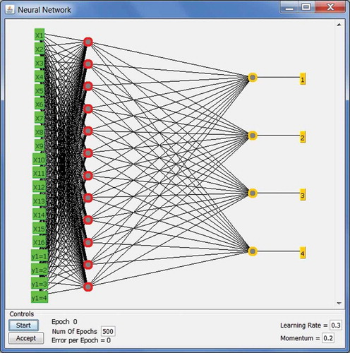
We used cross-validation with 100 replications to explore the (integer) values of the parameters k and h. From trial experiments, we concluded that the optimal results were obtained for values of k = 3 and h = 12, based on the average of accuracy, precision, recall, F1, and Hamming loss. All the results reported below relate to k = 3 and h = 12. Figure 8 shows a typology of ML-CA-LTM model with an input layer (with 16 inputs), one hidden layer (with 12 hidden units), and an output layer (with 4 outcomes).

Figure 8. Architecture of the ML-CA-LTM model (drivers X1 − X16 are explained in Table 2; cell states are agriculture (1), forest (2), industrial (3) and urban (4)).

Accuracy assessment

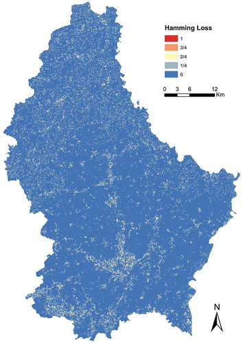
The accuracy assessment of the proposed model (Table 4) showed satisfactory results. In fact, the high accuracy, precision, recall, and F1 show that the model managed to capture the LUC patterns remarkably well and to adequately mimic the LUC function. The predicted land use for Luxembourg area in 2007 (Figure 9) is very similar to the real situation (i.e., reference land-use map in 2007) where the average of accuracy is 0.691 ± 0.021 (Table 4). This result clearly demonstrates the ability of the ML-CA-LTM model to capture the LUC patterns. Figure 10 shows an error map (Hamming loss), which is built from comparing observed and predicted maps in Figure 9. The error map or Hamming loss shows the difference between observed and predicted labels. According to the results, the overall Hamming loss is also low 0.131 ± 0.006 (Table 4).

Table 4. Assessing the performance of the ML-CA-LTM model.

Accuracy	Precision	Recall	F1	Hamming loss
0.691 ± 0.021	0. 799 ± 0.009	0.728 ± 0.012	0.843 ± 0.006	0.131 ± 0.006

Figure 9. Observed versus predicted land use in 2007.

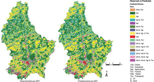
Figure 10. Map of hamming loss.

Figures 9 and 10 show that the new model could successfully predict the urban development and learned the changes to urban patterns. In fact, for decades, the majority of urban development took place in the central (city of Luxembourg) and southern (in specific southwest) parts of the outlining areas of Luxembourg. Moreover, the model proposed changes to urban areas that are characterized by low slope and were located near transport facilities. This is also in line with the observed changes (Figure 9).

A more detailed summary of the predictions is obtained by the confusion matrix for ML classification as shown in Figure 11. The rows and columns of this matrix are the ML (F, A, AF … AFIU) and its entries are the percentages of cells.

Figure 11. Confusion matrix with multi-labeling, observed versus predicted label set in 2007 (Note: normalized values between 0 and 100: each value in the original confusion matrix is divided by the sum of its corresponding line and multiplied by 100).

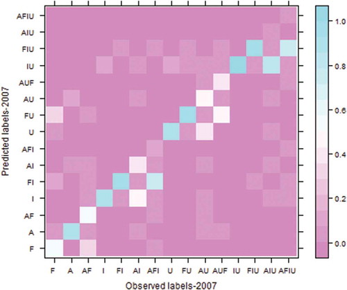
The label sets (A, AF, I, FI, AI) and (U, FU), (AUF, IU, FIU, AIU, AFIU) have been well predicted; however the label sets F, AI-AFI and AU have not been very well predicted as a result of complexity in the label set structure of land-use classes. For example, from Figure 11 we can easily see that the observed label set F (forest) is predicted mainly as label set F (forest) and label set FU (forest and urban). For the observed label set FI (forest and industrial), the ML-CA-LTM performed quite well. A big part of cells are correctly predicted as label set FI (forest and industrial) and few cells are classified as label set I (industrial), and label set FIU (forest, industrial, and urban). The label set AFI (agriculture, forest, and industrial) and AU (agriculture and urban) have been classified to (FI, AFI) and (AU, U), respectively. This is probably due to the high dependency/correlation among the label sets (e.g., AFI and FI). Indeed, the ML sets are more likely to be converted into other label sets.

As shown in Figure 11 and Table 5, the predicted and observed change matrices show that changes in land use occur more frequently in cells with more mixed land uses (i.e., containing more than one land-use class) than in cells with less mixed land uses. In fact, the more mixed the land use in a cell, the higher the probability that changes will occur in the land uses in the cell. For instance, cells containing two different land-use classes are more likely to change their states than cells containing only one land-use class. This is because cells associated with more than one land use (i.e., cells with mixed land uses) are located on the borders of the land uses. Expansion in a class of land use tends to start at the border area, so cells containing mixed land uses are generally the first to change state.

Table 5. Confusion matrix with mono-labeling, observed vs. predicted label set in 2007.

		Predicted label set in 2007
		U	I	A	F
Observed	U	741	69	354	100
	I	327	572	455	134
	A	132	87	296	436
	F	224	164	747	519

The ML-CA-LTM model managed to learn the interactions between different label sets, and this can be seen by comparing the two change matrices (Figure 11). For instance, cells containing urban and forestry or agricultural land uses are likely to gain industrial land uses when they change states. This is due to the fact that forestry and agricultural areas can easily be converted into areas of commerce and light industry. However, cells with urban, industrial, and agricultural or forestry areas (rows 14 and 1 in the change matrices) were found to lose their industrial uses, which means that old industrial plants are being abandoned. This might match reality because the economy of Luxembourg has changed from a reliance on steel and heavy industries to a reliance on the service sector (especially banking) in the last two decades. The predicted and observed changes both showed that agricultural land use is slowly losing out in favor of urban and forestry land uses. Further investigations are required to determine the influence of the presence of one class of land use on the development of another, and this can be achieved by performing a detailed assessment of the predicted and observed change matrices.

Model comparison

The comparison was made by using the procedure of learning and testing common in machine learning. We measured the performance of the proposed new model (ML-CA-LTM) and the standard LTM model, using standard evaluation measures adapted to ML learning. The model development was implemented in the computational language Matlab. The two methods, ML-CA-LTM and ml-CA-LTM that use two different approaches (i.e., ML and ml learning), were compared using common evaluation metrics, particularly the overall prediction accuracy, precision, recall and the F1-measure (Table 6). Based on the results shown in Table 6, the ML-CA-LTM model outperformed the ml-CA-LTM in all of the evaluation measures. The new model, based on BP-MLL, gave an accuracy (i.e., percentage of correctly classified instances) of 69.1%, whereas the ml-CA-LTM model gave a lower accuracy of 39.7%. The proposed model was also better at predicting all the land-use classes (see Table 6). In particular, the proposed ML-CA-LTM model predicted urban, industrial, agricultural, and forestland uses much more effectively than the ml-CA-LTM (conventional version of the LTM model with ML data), as can be seen from the accuracy, precision, and recall evaluation measures.

Table 6. Calculated accuracy metrics for ML-CA-LTM and ml-CA-LTM models (k = 3 and h = 12); based on 100 replications.

	ML-CA-LTM	ml-CA-LTM
Accuracy	0. 691 ± 0.021	0.397 ± 0.009
Precision	0. 799 ± 0.009	0.464 ± 0.009
Recall	0.728 ± 0.012	0.397 ± 0.009
F1	0.843 ± 0.006	0.414 ± 0.009
Accuracy [U]	0.885 ± 0.015	0.586 ± 0.009
Accuracy [I]	0.827 ± 0.016	0.384 ± 0.009
Accuracy [A]	0.917 ± 0.012	0.311 ± 0.009
Accuracy [F]	0.850 ± 0.011	0.314 ± 0.009
Precision [U]	0.578 ± 0.047	0.520 ± 0.009
Precision [I]	0.496 ± 0.053	0.641 ± 0.009
Precision [A]	0.935 ± 0.018	0.160 ± 0.009
Precision [F]	0.870 ± 0.020	0.437 ± 0.009
Recall [U]	0.710 ± 0.045	0.586 ± 0.009
Recall [I]	0.359 ± 0.083	0.384 ± 0.009
Recall [A]	0.961 ± 0.016	0.311 ± 0.009
Recall [F]	0.864 ± 0.019	0.314 ± 0.009
Build_time (seconds)	10.866 ± 0.106	5.69 ± 0.305

Discussion

This paper presents an original modeling framework that permits ML class assignment in land use using LTM land use models and CA. The BP-MLL was used to identify the CA transition rules. It has been shown in several applications that an ML modeling framework has potential gain over ml learning (Yang et al. 2012). In land change science, we showed that the ML models are more efficient than ml models since additional information regarding the labels present in a cell is exploited (prior information about label dependence). The concept of ML can be incorporated in other well-known land change models as well (e.g., SLEUTH, CLUE, GEOMOD, Geo-Simulation, and others).

Another important point to discuss is the generation of ML land-use data. In this paper, we converted vector maps to raster images using a soft classification allowing a cell to have more than one land-use class. As a result, a cell may be associated with several labels, for instance, when it is on the border of residential and industrial areas, although a piece of land may have genuinely mixed-use. There are other ways according to the needs and the purpose of the application. For instance, we mention hereafter two possible and easy ways, among others, to build ML data in land-use science. First, we can create ML land-use data from raster grids (SPOT images) with high resolution (e.g., 10 or 20 m) and then aggregate it at a coarser scale (e.g., 100 m). The later resolution is suitable to detect variability that can be partially diminished at finer resolutions (White and Engelen 2000). Second, it is also possible to assign two different categorical variables to each cell as an ML outcome. For example, a cell can be classified as “urban” or “non-urban” and in the same time as “low density of population,” “high density of population,” or “no population.” This structure of categorical variables, as proposed by White, Uljee, and Engelen (2012) using an activity-based model, is different from our proposal. The current work applied the concept of ML class assignment in land change science which is different from modeling multiple LUCs (Tayyebi and Pijanowski 2014). The current model can handle ML data and predict ML land-use status (Omrani et al. 2015a).

The current paper limited the land-use characteristics to few drivers such as slope, neighbors, and distance from highway and networks (bus and train stations) due to the data limitation access in Luxembourg. These factors were used extensively by many researchers to explain the LUC processes (e.g., Pijanowski et al. 2014; De Almeida et al. 2003; Verburg et al. 2002; Basse et al., 2014). Adding more demographic, economic, planning, and policy factors may improve the performance of the ML-CA-LTM model. These variables (e.g., population, jobs, housing prices, mobility flow, and accessibility) are often defined at a macro scale (e.g., municipality) and will need to be disaggregated down to a microlevel (i.e., cell level). Moreover, the proposed model did not integrate the proportion of each land-use class. Therefore, the ML-CA-LTM can be extended in the future to take into account these issues. The proposed modeling framework will open diverse perspectives of research on both theoretical and empirical sides (such as modeling and evaluation issues, big data and cloud computing, and data analytics) having exciting challenges as given in the next section.

Conclusion

In this study, we suggested a new algorithm for modeling mixed LUCs. ML-CA-LTM presents the spatial unit in an intuitive way as it allows them to have more than one land-use class at the same time. It also allows the modeling of interaction among different combinations of land-use classes. ML-CA-LTM derives the functional relationships between mixed LUC and a set of explanatory variables. The BP-MLL was used to identify the transition rules of CA. We validated the integrated model using the popular evaluation measures, accuracy, precision, recall and F1-measure, adapted to ML learning for a case study in Luxembourg. The ML-CA-LTM had promising results and managed to mimic the LUCs complexity well. As a summary, we reached the following conclusions for Luxembourg and similar locations undergoing LUC:

1. The ml-CA-LTM model is not an effective tool to predict mixed LUC. It uses a binary transformation method (with the BP neural network algorithm commonly used in the LTM model for ml learning) and so it ignores the dependence among labels.

2. The ML-CA-LTM is an efficient tool to predict mixed LUC, with nonexclusive LU classes.

There are many areas that need further research. First, future work is needed to solve the class imbalance problem (certain labels are more abundant than others) to avoid the misclassification of the less common classes of land use. Second, variables for population, economic growth, zoning, planning, and policy factors could be added to demonstrate the usability of the model, to control, provide bounds, and better forecast changes in land use. Last but not least, other ML learning models should be considered (e.g., support vector machine, decision tree, logistic regression, instance-based learning or nearest neighbors, among many others) for simulating mixed LUC.

Highlights

• We applied the multi-label concept in which a unit may have several elementary labels.

• We integrated Land Transformation Model with a cellular automata model to simulate multi-label or mixed land use changes.

• The new model performed better in capturing mixed land-use patterns.

• The outcome of modified model can be used by managers and decision makers for urban planning.

Acknowledgments

This research work has been carried out at the Center for Global Soundscapes at Purdue University. The authors would like to acknowledge the ML-CA-LTM project co-funded by the LISER research institute (for granting me six months’ scientific leave from fall 2016) and the National Research Fund Luxembourg (FNR). BCP was supported by the USDA McIntire-Stennis Cooperative Forestry Program and Purdue University. Dr. Omrani is grateful to Ms. Bellisario, Kristen M (PhD student at the Department of Forestry and Natural Resources, Purdue University-USA) for editing the final version of the manuscript. The authors are thankful for three reviewers as well the editor of their valuable comments and suggestions concerning various versions of the manuscript.

Disclosure statement

No potential conflict of interest was reported by the authors.

Additional information

Funding

This work was supported by the LISER research institute; National Research Fund Luxembourg; USDA McIntire-Stennis Cooperative Forestry Program; Purdue University.

References

- Akın, A., K. C. Clarke, and S. Berberoglu. 2014. “The Impact of Historical Exclusion on the Calibration of the SLEUTH Urban Growth Model.” International Journal of Applied Earth Observation and Geoinformation 27: 156–168. doi:10.1016/j.jag.2013.10.002.
- Azari, M., A. Tayyebi, M. Helbich, and M. A. Reveshty. 2016. “Integrating Cellular Automata, Artificial Neural Network, and Fuzzy Set Theory to Simulate Threatened Orchards: Application to Maragheh, Iran.” Giscience & Remote Sensing 53 (2): 183–205.
- Bagan, H., and Y. Yamagata. 2015. “Analysis of Urban Growth and Estimating Population Density Using Satellite Images of Nighttime Lights and Land-Use and Population Data.” Giscience & Remote Sensing 52 (6): 765–780. doi:10.1080/15481603.2015.1072400.
- Basse, R. M., H. Omrani, O. Charif, P. Gerber, and K. Bódis. 2014. “Land Use Changes Modelling Using Advanced Methods: Cellular Automata and Artificial Neural Networks. the Spatial and Explicit Representation of Land Cover Dynamics at the Cross-Border Region Scale.” Applied Geography 53: 160–171. doi:10.1016/j.apgeog.2014.06.016.
- Batty, M. 2011. “Modeling and Simulation in Geographic Information Science: Integrated Models and Grand Challenges.” Procedia-Social and Behavioral Sciences 21: 10–17. doi:10.1016/j.sbspro.2011.07.003.
- Blecic, I., A. Cecchini, and G. A. Trunfio. 2013. “Cellular Automata Simulation of Urban Dynamics through GPGPU.” The Journal of Supercomputing 65 (2): 614–629. doi:10.1007/s11227-013-0913-z.
- Boutell, M. R., J. Luo, X. Shen, and C. M. Brown. 2004. “Learning Multi-Label Scene Classification.” Pattern Recognition 37 (9): 1757–1771. doi:10.1016/j.patcog.2004.03.009.
- Brown, D. G., P. H. Verburg, R. G. Pontius, and M. D. Lange. 2013. “Opportunities to Improve Impact, Integration, and Evaluation of Land Change Models.” Current Opinion in Environmental Sustainability 5 (5): 452–457. doi:10.1016/j.cosust.2013.07.012.
- Clarke, K., S. Hoppen, and L. Gaydos. 1997. “A Self-Modifying Cellular Automaton Model of Historical Urbanization in the San Francisco Bay Area.” Environment and Planning B: Planning and Design 24: 247–261. doi:10.1068/b240247.
- Couclelis, H. 2005. “Where Has the Future Gone? Rethinking the Role of Integrated Land-Use Models in Spatial Planning.” Environment and Planning A 37: 1353–1371. doi:10.1068/a3785.
- De Almeida, C. M., M. Batty, A. M. V. Monteiro, G. Câmara, B. S. Soares-Filho, G. C. Cerqueira, and C. L. Pennachin. 2003. “Stochastic Cellular Automata Modeling of Urban Land Use Dynamics: Empirical Development and Estimation.” Computers, Environment and Urban Systems 27 (5): 481–509. doi:10.1016/S0198-9715(02)00042-X.
- Farr, T., P. A. Rosen, E. Caro, R. Crippen, R. Duren, S. Hensley, M. Kobrick, et al. 2007. “The Shuttle Radar Topography Mission.” Reviews of Geophysics 45 (2). doi:10.1029/2005RG000183.
- Grekousis, G., P. Manetos, and Y. N. Photis. 2013. “Modeling Urban Evolution Using Neural Networks, Fuzzy Logic and GIS: The Case of the Athens Metropolitan Area.” Cities 30: 193–203. doi:10.1016/j.cities.2012.03.006.
- Heaton, J. 2005. Introduction to Neural Networks with Java. Chesterfield: Heaton Research.
- Hijmans, R. J., S. E. Cameron, J. L. Parra, P. G. Jones, and A. Jarvis. 2005. “Very High Resolution Interpolated Climate Surfaces for Global Land Areas.” International Journal of Climatology 25 (15): 1965–1978. doi:10.1002/(ISSN)1097-0088.
- Huang, B., C. Xie, and R. Tay. 2010. “Support Vector Machines for Urban Growth Modeling.” Geoinformatica 14: 83–99. doi:10.1007/s10707-009-0077-4.
- Lambin, E. F., and H. J. Geist. eds. 2006. Land-Use and Land-Cover Change: Local Processes and Global Impacts, 222 pp. The IGBP Global Change Series. Berlin: Springer-Verlag.
- Lambin, E. F., B. L. Turner, H. J. Geist, S. B. Agbola, A. Angelsen, J. W. Bruce, O. T. Coomes, T. A. Veldkamp, C. Vogel, J. Xu. 2001. “The Causes of Land-Use and Land-Cover Change: Moving beyond the Myths.” Global Environmental Change 11 (4): 261–269. doi:10.1016/S0959-3780(01)00007-3.
- Li, X., and A. Yeh. 2001. “Calibration of Cellular Automata by Using Neural Networks for the Simulation of Complex Urban Systems.” Environment and Planning A 33: 1445–1462. doi:10.1068/a33210.
- Li, X., and A. Yeh. 2002. “Neural-Network-Based Cellular Automata for Simulating Multiple Land Use Changes Using Gis.” International Journal of Geographical Information Science 16: 323–343. doi:10.1080/13658810210137004.
- Malczewski, J. 2006. “Ordered Weighted Averaging with Fuzzy Quantifiers: GIS-Based Multicriteria Evaluation for Land-Use Suitability Analysis.” International Journal of Applied Earth Observation and Geoinformation 8 (4): 270–277. doi:10.1016/j.jag.2006.01.003.
- Maps. 1999. Land Cover [Map].Scale: 1:10.000. Owned by Ministry of Environment Luxembourg.
- Maps. 2007. Land Cover [Map].Scale: 1:10.000. Owned by Ministry of Environment Luxembourg.
- Mas, J. F., H. Puig, J. L. Palacio, and A. Sosa-López. 2004. “Modelling Deforestation Using GIS and Artificial Neural Networks.” Environmental Modelling & Software 19: 461–471. doi:10.1016/S1364-8152(03)00161-0.
- Mustard, J. F., R. S. Defries, T. Fisher, and E. Moran. 2004. “Land-Use and Land-Cover Change Pathways and Impacts.” In Land Change Science, 411–429. Netherlands: Springer.
- Olson, J. M., G. Alagarswamy, J. A. Andresen, D. J. Campbell, A. Y. Davis, J. Ge, B. C. Pijanowski, and J. Wang. 2008. “Integrating Diverse Methods to Understand Climate–Land Interactions in East Africa.” Geoforum 39 (2): 898–911. doi:10.1016/j.geoforum.2007.03.011.
- Omrani, H., F. Abdallah, O. Charif, and N. T. Longford. 2015a. “Multi-Label Class Assignment in Land-Use Modelling.” International Journal of Geographical Information Science 29 (6): 1023–1041. doi:10.1080/13658816.2015.1008004.
- Omrani, H., O. Charif, P. Gerber, A. Awasthi, and P. Trigano. 2013. “Prediction of Individual Travel Mode with Evidential Neural Network Model.” Transportation Research Record: Journal of the Transportation Research Board 2399 (2399): 1–8. doi:10.3141/2399-01.
- Omrani, H., A. Tayyebi, and B. C. Pijanowski. 2015b. “Integrating the Multi-Label Land Use Concept and Cellular Automata with the ANN-Based Land Transformation Model.” In Geocomputing Conference, 208–210. Dallas, TX: The University of Texas.
- Pijanowski, B., D. K. Ray, A. D. Kendall, J. M. Duckles, and D. W. Hyndman. 2007. “Using Back-Cast Land-Use Change and Groundwater Travel Time Models to Generate Land-Use Legacy Maps for Watershed Management.” Ecology and Society 12 (2): 25. doi:10.5751/ES-02154-120225.
- Pijanowski, B. C., K. Alexandridis, and D. Mueller. 2006. “Modelling Urbanization Patterns in Two Diverse Regions of the World.” Journal of Land Use Science 1 (2–4): 83–108. doi:10.1080/17474230601058310.
- Pijanowski, B. C., G. Daniel, S. Brown, and A. Manik. 2002a. “Using Neural Networks and GIS to Forecast Land Use Changes: A Land Trans- Formation Model.” Computers, Environment and Urban Systems 26: 553–575. doi:10.1016/S0198-9715(01)00015-1.
- Pijanowski, B. C., B. Shellito, S. Pithadia, and K. Alexandridis. 2002b. “Forecasting and Assessing the Impact of Urban Sprawl in Coastal Watersheds along Eastern Lake Michigan.” Lakes & Reservoirs: Research & Management 7 (3): 271–285. doi:10.1046/j.1440-1770.2002.00203.x.
- Pijanowski, B. C., A. Tayyebi, M. R. Delavar, and M. J. Yazdanpanah. 2009. “Urban Expansion Simulation Using Geographic Information Systems and Artificial Neural Networks.” International Journal Environment Researcher 3 (4): 493–502.
- Pijanowski, B. C., A. Tayyebi, J. Doucette, B. K. Pekin, D. Braun, and J. Plourde. 2014. “A Big Data Urban Growth Simulation at A National Scale: Configuring the GIS and Neural Network Based Land Transformation Model to Run in A High Performance Computing (HPC) Environment.” Environmental Modelling & Software 51: 250–268. doi:10.1016/j.envsoft.2013.09.015.
- Power, C., A. Simms, and R. White. 2001. “Hierarchical Fuzzy Pattern Matching for the Regional Comparison of Land Use Maps.” International Journal of Geographical Information Science 15 (1): 77–100. doi:10.1080/136588100750058715.
- Ray, D. K., B. C. Pijanowski, A. D. Kendall, and D. W. Hyndman. 2012. “Coupling Land Use and Groundwater Models to Map Land Use Legacies: Assessment of Model Uncertainties Relevant to Land Use Planning.” Applied Geography 34: 356–370. doi:10.1016/j.apgeog.2012.01.002.
- Reed, R. D., and R. J. Marks. 1998. Neural Smithing: Supervised Learning in Feedforward Artificial Neural Networks. Cambridge, MA: MIT Press.
- Rindfuss, R. R., S. J. Walsh, B. L. Turner, J. Fox, and V. Mishra. 2004. “Developing a Science of Land Change: Challenges and Methodological Issues.” Proceedings of the National Academy of Sciences of the United States of America 101 (39): 13976–13981. doi:10.1073/pnas.0401545101.
- Shan, J., S. Alkheder, and J. Wang. 2008. “Genetic Algorithms for the Calibration of Cellular Automata Urban Growth Modeling.” Photogrammetric Engineering & Remote Sensing 74 (10): 1267–1277. doi:10.14358/PERS.74.10.1267.
- Sorower, M. S. 2010. A Literature Survey on Algorithms for Multi-Label Learning. Corvallis: Oregon State University.
- Tayyebi, A., B. K. Pekin, B. C. Pijanowski, J. D. Plourde, J. S. Doucette, and D. Braun. 2013. “Hierarchical Modeling of Urban Growth across the Conterminous USA: Developing Meso-Scale Quantity Drivers for the Land Transformation Model.” Journal of Land Use Science 8 (4): 422–442. doi:10.1080/1747423X.2012.675364.
- Tayyebi, A., P. C. Perry, and A. H. Tayyebi. 2014a. “Predicting the Expansion of an Urban Boundary Using Spatial Logistic Regression and Hybrid Raster–Vector Routines with Remote Sensing and GIS.” International Journal of Geographical Information Science 28 (4): 639–659. doi:10.1080/13658816.2013.845892.
- Tayyebi, A., and B. C. Pijanowski. 2014. “Modeling Multiple Land Use Changes Using ANN, CART and MARS: Comparing Tradeoffs in Goodness of fit and Explanatory Power of Data Mining Tools.” International Journal of Applied Earth Observation and Geoinformation 28: 102–116. doi:10.1016/j.jag.2013.11.008.
- Tayyebi, A., B. C. Pijanowski, M. Linderman, and C. Gratton. 2014b. “Comparing Three Global Parametric and Local Non-Parametric Models to Simulate Land Use Change in Diverse Areas of the World.” Environmental Modelling & Software 59: 202–221. doi:10.1016/j.envsoft.2014.05.022.
- Turner, B. L., E. F. Lambin, and A. Reenberg. 2007. “The Emergence of Land Change Science for Global Environmental Change and Sustainability.” Proceedings of the National Academy of Sciences 104 (52): 20666–20671. doi:10.1073/pnas.0704119104.
- Verburg, P. H., W. Soepboer, A. Veldkamp, R. Limpiada, V. Espaldon, and S. S. Mastura. 2002. “Modeling the Spatial Dynamics of Regional Land Use: the CLUE-S Model.” Environmental Management 30 (3): 391–405. doi:10.1007/s00267-002-2630-x.
- Washington-Ottombre, C., B. Pijanowski, D. Campbell, J. Olson, J. Maitima, A. Musili, T. Kibaki, H. Kaburu, P. Hayombe, E. Owango, B. Irigia. 2010. “Using a Role-Playing Game to Inform the Development of Land-Use Models for the Study of a Complex Socio-Ecological System.” Agricultural Systems 103 (3): 117–126. doi:10.1016/j.agsy.2009.10.002.
- Wayland, K. G., D. T. Long, D. W. Hyndman, B. C. Pijanowski, S. M. Woodhams, and S. K. Haack. 2003. “Identifying Relationships between Baseflow Geochemistry and Land Use with Synoptic Sampling and R-Mode Factor Analysis.” Journal of Environment Quality 32 (1): 180–190. doi:10.2134/jeq2003.1800.
- White, R., and G. Engelen. 2000. “High-Resolution Integrated Modelling of the Spatial Dynamics of Urban and Regional Systems.” Computers, Environment and Urban Systems 24: 383–400. doi:10.1016/S0198-9715(00)00012-0.
- White, R., I. Uljee, and G. Engelen. 2012. “Integrated Modelling of Population, Employment and Land-Use Change with a Multiple Activity-Based Variable Grid Cellular Automaton.” International Journal of Geographical Information Science 26: 1251–1280. doi:10.1080/13658816.2011.635146.
- Witten, I. H., and E. Frank. 2005. Data Mining: Practical Machine Learning Tools and Techniques, 2nd ed. San Francisco, CA: Morgan Kaufmann.
- Wolfram, S. 1994. Cellular Automata and Complexity: Collected Papers (Vol. 1). Reading: Addison-Wesley.
- Wolfram, S. 2002. A New Kind of Science (Vol. 5). Champaign: Wolfram media.
- Yang, Q., X. Li, and X. Shi. 2008. “Cellular Automata for Simulating Land Use Changes Based on Support Vector Machines.” Computers & Geosciences 34: 592–602. doi:10.1016/j.cageo.2007.08.003.
- Yang, Q., J. Shao, M. Scholz, C. Boehm, and C. Plant. 2012. “Multi-Label Classification Models for Sustainable flood Retention Basins.” Environmental Modelling & Software 32: 27–36. doi:10.1016/j.envsoft.2012.01.001.
- Zhang, M. L., and Z. H. Zhou. 2006. “Multilabel Neural Networks with Applications to Functional Genomics and Text Categorization.” IEEE Transactions on Knowledge and Data Engineering 18 (10): 1338–1351. doi:10.1109/TKDE.2006.162.