From ERS-1/2 to Sentinel-1: two decades of subsidence monitored through A-DInSAR techniques in the Ravenna area (Italy)

Abstract

Land subsidence due to underground resources exploitation is a well-known problem that affects many cities in the world, especially the ones located along the coastal areas where the combined effect of subsidence and sea level rise increases the flooding risk. In this study, 25 years of land subsidence affecting the Municipality of Ravenna (Italy) are monitored using Advanced Differential Interferometric Synthetic Aperture Radar (A-DInSAR) techniques. In particular, the exploitation of the new Sentinel-1A SAR data allowed us to extend the monitoring period till 2016, giving a better understanding of the temporal evolution of the phenomenon in the area. Two statistical approaches are applied to fully exploit the informative potential of the A-DInSAR results in a fast and systematic way. Thanks to the applied analyses, we described the behavior of the subsidence during the monitored period along with the relationship between the occurrence of the displacement and its main driving factors.

Keywords:

• InSAR
• Sentinel-1
• subsidence
• Ravenna
• time series

1. Introduction

Differential Synthetic Aperture Radar Interferometry (DInSAR) is a very powerful remote sensing tool able to measure the displacements on the Earth surface with millimetric accuracy. The first description of DInSAR was given by Gabriel, Goldstein, and Zebker (1989), and it was successfully applied for the first time as a ground-motion detection technique in the early 1990s with the study of the Landers earthquake in California and the Mount Etna volcano in Italy (Massonnet et al. 1993, 1995). This method uses the phase shift between two radar acquisitions (SAR images) made over the same place at different times to generate an interferogram and calculate the ground deformation. The interferometric phase (Δφ) is made by different contributions:

where Δφ_topo is the contribution given by the topography, Δφ_def is the contribution given by the deformation, Δφ_orb is the phase given by uncompensated difference in the satellite’s orbits, Δφ_atm is the phase component given by atmospheric effects, and Δφ_noise is the systematic noise. One of the main advantages of the DInSAR approach is that the topographic component of the phase (Δφ_topo) is reduced using an external Digital Elevation Model (DEM) providing (qualitative) information on deformations, even with a reduced SAR data availability (Cascini, Fornaro, and Peduto 2010). On the other hand, the main drawback is that analyzing just one interferogram is not possible to remove the strong atmospheric disturbance that inevitably lead to inaccuracies in the detected movements, limiting its operational capability (Cascini, Fornaro, and Peduto 2010). Furthermore, since DInSAR can only measure the total displacement between two points in time, it cannot distinguish between linear and nonlinear motion. Hence, in order to cope with these limitations, a new class of DInSAR techniques called Persistent Scatterers Interferometry (PSI) was developed. In this work, we refer to PSI with the term Advanced DInSAR (A-DInSAR). There are two main A-DInSAR techniques: the Permanent Scatterers (PS) (Ferretti, Prati, and Rocca 2000, 2001) and the Small BAseline Subset (SBAS) (Berardino et al. 2002). These techniques exploit the information of multiple SAR acquisitions made over the same area to estimate and reduce the effects given by decorrelation phenomena and atmospheric phase shifts obtaining very accurate deformation measures over time. The PS technique analyses at full resolution dominant point scatterers (PSs) that maintain phase stability over long periods. Any phase disturbance such as atmospheric artifacts and topographic inaccuracies are estimated and compensated retrieving the precise displacement of the PSs. Since PSs density is generally higher in urban environments, this technique is more suitable for ground deformation analysis in metropolitan areas (Soergel 2010). The SBAS techniques rely on the combination of interferometric pairs with small temporal and perpendicular baselines to measure the deformation of distributed scatterers. To enhance phase stability, a multi-look factor in range and azimuth is generally adopted but this leads to a reduced spatial resolution. The application of SBAS is more suited over large areas, where the absence of a high number of stable reflectors limits the applicability of the PS approach. For this reason, SBAS is widely used for Earth Observation purposes in several scenarios, such as low-vegetated land, sparsely urbanized territory, and coastal areas. A-DInSAR has proven to be one of the most reliable tool for the detection and monitoring of different geological hazards such as earthquakes (Chini et al. 2016), landslides (Di Martire et al. 2016), subsidence (Tessitore et al. 2016), and volcanic activity (Meyer et al. 2015), and is nowadays widely used to map ground deformations due to natural and anthropogenic processes in different environments. Furthermore, one of the main advantages is the possibility to reconstruct the past behavior of the displacement using archive data and perform time series analyses. This is useful in particular in the framework of geological hazard risk assessment and territory management; in fact, thanks to the analysis of the ground instability evolution, it is possible to understand its cause-effect mechanism and to evaluate the most feasible corrective measures (Tomás et al. 2005). While the monitoring of geological hazards with conventional ground-based techniques (e.g. inclinometers, leveling, Global Positioning System) is usually expensive and time consuming, A-DInSAR techniques permit to reduce operating costs and working time especially when used for large-scale surveys. Despite the great benefits brought by the application of radar interferometry to the geological hazard monitoring, the exploitation of very large SAR datasets can produce huge amounts of data that are often difficult to properly manage and interpret. Statistical methods can be applied to analyze the A-DInSAR processing results to fully exploit their informative content.

In this work, we present the outcomes in monitoring the land subsidence affecting the Municipality of Ravenna with 25 years of SAR data, starting from 1992 with the ERS-1/2 and ending with the 2016 Sentinel-1A images. The obtained results are then cross-validated comparing two different A-DInSAR approaches, the SBAS and the Coherent Pixel Technique (CPT) (Mora, Mallorqui, and Broquetas 2003; Iglesias, Mallorqui, and Lopez-Dekker 2014). Furthermore, we show the application of a new methodology based on statistical analyses to manage in a systematic way the obtained results and better describe the behavior of the subsidence during the monitoring period along with the relationship between the occurrence of the displacement and its main driving factors.

The main aims of this work are: (i) to monitor the land subsidence affecting the territory of Ravenna using A-DInSAR techniques and extend the observed period to 2016 with the new Sentinel-1A satellite; (ii) to understand the subsidence trends over the 25 years period and determine which are the main controlling factors through the application of statistical analyses; (iii) to compare and cross-validate the results obtained through two different A-DinSAR approaches and demonstrate the reliability of the measured subsidence rates; (iv) to assess the capabilities of the Sentinel-1A sensor in the monitoring of sparsely urbanized areas.

2. Study area

The city of Ravenna is located in the Emilia Romagna Region (northeast of Italy), where land subsidence of natural and anthropogenic origin occurs since the last century (Teatini et al. 2005). One of the main causes of the subsidence in the area is the overexploitation of the methane gas and water reservoirs that started in the 1940s along with the industrial growth and gradually reduced around the 1980s (Gambolati et al. 1999). Concerned by the very high values of subsidence registered, the Municipality of Ravenna started in the late 1970s the construction of a new public aqueduct to exploit the surface water that led to a reduced aquifer overdraft (Gambolati et al. 1999). Today, even if the ratio of the anthropogenic subsidence (<−20 mm/year) lowered a lot in respect to the previous decades, it is still 10 times higher than the natural one (−2 mm/year) (Gambolati et al. 1991). This represents a serious threat in particular for the coastal areas where the subsidence effect added to the mean sea level rise increases the flooding risk (Carbognin and Tosi 2002).

2.1. Geological settings

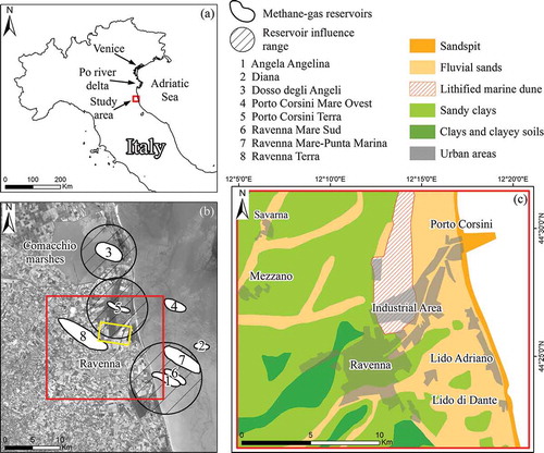
The territory of Ravenna (Figure 1(a)) lies over the southeastern portion of the Po River plain, an area of about 38,000 km² bounded by the Alps in the north and the Apennines in the south (Teatini et al. 2005). The buried tectonic structures underlain around 2000 m of Quaternary sediments of Alpine and Apennines origin deposited under different environments, from continental to marine (Amorosi et al. 1999; Carminati, Martinelli, and Severi 2003; Ghielmi et al. 2010). The pre-Quaternary basement is characterized by a complex structure of folds and faults that develop parallel to the main Apennine tectonic lines forming natural traps for the methane gas (Gambolati et al. 1991). Several Pliocene and Pleistocene gas fields are located in thrusted anticlines, with depths ranging between 1000 and 4500 m, simple drape structures, and stratigraphic traps. The Quaternary sequence is made of normally consolidated layers of alternating silty clay, sand, and sandy silt (Figure 1(c)). A multi-layer acquifer system developed in the first 500 m of sediments accumulated since the Pleistocene. This system is characterized by sediments deposited during transgressive and regressive stages.

Figure 1. (a) Location of the study area; (b) Methane gas reservoirs close to Ravenna. The yellow square is the area used for the cross-validation between the SBAS and CPT results. Basemap: 18 July 2016 Sentinel-2 image; (c) Geological map of the study area and main locations. For full colour versions of the figures in this paper, please see the online version.

2.2. Mechanisms of the subsidence

The subsidence affecting the Adriatic Sea coastline in northern Italy can be related to different anthropic and natural factors that vary locally: tectonic, glacial isostatic adjustment, reclaimed peatland oxidation, groundwater withdrawal, gas extraction, natural sediments compaction. The Regional Agency for the Environmental Protection (ARPA) of Emilia-Romagna Region and the Emilia-Romagna Region (2010) estimate the overall contribution of the natural subsidence in −1.4 mm/year at Ravenna, −2.5 mm/year at Po river delta, and −1 mm/year at Venice. Gambolati et al. (1999) also modeled and calculated the natural subsidence due to sediments compaction with rates of −2.5 mm/year at Ravenna, −4 to −5 mm/year in the Po river delta, and 0.5 mm/year at Venice. The present-day subsidence in the Po Plain is also given by the effects of the last deglaciation period that contributes with increasing values going from Venice (−1.1 mm/year) to Ravenna (−3.5 mm/year) (Carminati, Martinelli, and Severi 2003). At regional scale, the main cause of the anthropogenic subsidence can be related to the combined effects of the extraction of underground water and methane gas from on and offshore reservoirs. At local scale, in particular along the coastline close to Ravenna, the high rates of subsidence are more related to the exploitation of the offshore methane gas fields closer to the shoreline (ENI and ARPA 2003)

2.2.1. Subsidence due to methane gas extraction

In the Ravenna area, there are eight main gas fields (Figure 1(b)), five of which are offshore and three onshore. The production that started in the 1970s is still ongoing at the present day for most of the fields: only two fields are inactive, Ravenna Terra and Porto Corsini Terra, which exploitation stopped in 1992 and 2014, respectively. The most productive fields are Dosso degli Angeli and Angela-Angelina, with average annual production from 1980 to 2016 of 450 × 10⁶ Sm³ and 600 × 10⁶ Sm³, respectively (http://unmig.mise.gov.it/).

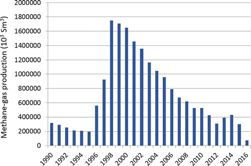
Angela-Angelina gas field is one of the major reservoirs in Northern Adriatic. The production started in 1973 and is still active. Due to its proximity to the coastline (around 2 km), and the high productivity rates (Figure 2), the impact on the coastline produced by the depletion of the reservoirs can be much higher than the one of the other gas fields (Gambolati et al. 1999). Gambolati and Teatini (1998) simulated the subsidence caused by the reservoir compaction and estimated a maximum influence range of around 6.5 km (Figure 1(b)).

Figure 2. Production rate of the Angela-Angelina methane gas field for the period 1990–2016.

Dosso degli Angeli is an onshore gas field located under the Comacchio Marshes, 20 km North of Ravenna. From the beginning of the production until 2004, the reservoir produced 30 × 10⁹ Sm³ of methane gas. The average annual production was constant until 1990 with more than 1 × 10⁹ Sm³. Afterwards, it slowly decreased till ending in 2004. In 2011, the production started again with an average annual production of 100 × 10⁶ Sm³. ARPA (2010), estimated in 5 km the influence range of the reservoir.

The Porto Corsini Terra gas field is located 6 km northeast of Ravenna. From 1980 until 2014, the average annual production was 20 × 10⁶ Sm³. Bertoni et al. (1995) estimated a maximum influence range of about 5.5 km (Figure 1(b)).

2.2.2. Subsidence due to groundwater extraction

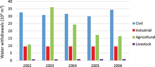
Another anthropogenic component of the subsidence affecting the study area is related to the water extraction activities. Since the water withdrawal rate is strongly dependent on different factors among which the number of used wells, the depth and geology of the exploited reservoirs, and the climate, the subsidence rates vary locally. The water use in the Region can be divided in four main categories: civil, industrial, agricultural, and livestock. According to ARPA (2010), from 2002 to 2006 the simulated water withdrawals, in millions of m³/year, were: 32 for civil use, 10 for industrial use, and 1 for livestock use (Figure 3). The water extraction rates for agricultural use are more variable because of its relationship with the climatic and seasonal conditions. The rates vary from 36 × 10⁶ m³/year to 10 × 10⁶ m³/year. Most of the withdrawals (1.72 m³/s) for all the categories take place at depth ranging from −40 m to −100 m. Among these, the 54% of the extractions (0.94 m³/s) are from −10 m to −40 m. Only the extractions for industrial use take place in the deeper reservoirs ranging from −200 m to −340 m of depth.

Figure 3. Groundwater withdrawals in millions of m³ calculated for each type of well for the period 2002–2006, redrawn from ARPA (2010) (http://www.arpae.it/).

3. Methodology

3.1. A-DInSAR processing and available datasets

A-DInSAR techniques permit to obtain reliable deformation time series for the pixels that present good phase quality. The latter can be low due to geometrical and temporal decorrelation phenomena occurring in the interferograms. Therefore, a preliminary pixel selection is necessary to obtain trustworthy processing results. The pixel phase quality analysis can be carried out following three main criteria: (1) coherence stability (Berardino et al. 2002; Mora, Mallorqui, and Broquetas 2003; Lanari et al. 2004); (2) amplitude dispersion index (Ferretti, Prati, and Rocca 2001); (3) temporal sublook spectral coherence (Iglesias, Mallorqui, and Lopez-Dekker 2014). In the first case (1), the pixels are chosen considering their mean coherence computed using all the multi-looked interferograms. Such pixel coherence is a function of the interferometric phase’s standard deviation (Blanco et al. 2006). The displacement information is then calculated choosing a coherence threshold value, only for the pixels that present a high interferometric quality. The amplitude dispersion index (2) permits to select pixels with a stable electromagnetic response (when their signal-to-noise ratio is high). The latter method (3), applies a point-like coherent scatterers selection, taking into account the temporal axis.

In the present work, A-DInSAR techniques have been used to get 25 years (1992–2016) of ground displacement monitoring in the Ravenna Municipality area exploiting four SAR datasets acquired by C- and X-band satellites. To this aim, the SBAS and CPT algorithms, respectively, implemented in the SARscape® and SUBSOFT processor software packages have been used. Specifically, 57 ERS-1/2 (C-band), 60 ENVISAT (C-band), 53 TerraSAR-X StripMap (X-band) and 30 Sentinel-1A Interferometric Wide Swath (C-band) images acquired in descending geometry have been processed with SARscape®. The main features of each dataset and their temporal coverage have been reported in Table 1. The processing window adopted (study area) is 18 km × 21 km focusing the monitoring activity on the city of Ravenna and its shoreline (Figure 1(b)). The SUBSOFT processor has been used to process only the ENVISAT and TerraSAR-X datasets over a smaller area (6 km × 3 km) in the industrial area of Ravenna (Figure 1(b)), in order to perform the comparison analyses between the two different approaches and cross-validate the results.

Table 1. Details of the available SAR image datasets.

Satellite	ERS-1/2	ENVISAT	TerraSAR-X	Sentinel-1A
Period covered	10 May 1992– 13 December 2000	02 April 2003– 22 September 2010	25 February 2012– 05 April 2014	12 October 2014– 11 January 2016
Track No.	122	122	2	95
Number of images	57	60	53	30
Wavelength (cm)	5.6	5.6	3	5.6
Incidence angle (°)	23	23	29	39
Imaging mode	SAR	ASAR IM	StripMap	Wide Swath
Polarization	VV	VV	HH	VV

The SBAS processing workflow adopted in SARscape® consists of five main steps: (a) connection graph (CG) generation; (b) interferogram generation and unwrapping; (c) refinement and re-flattening; (d) first and second inversion; and (e) geocoding. In the first step (a), the connection links between master and slaves image pairs are created based on the specified temporal and perpendicular baseline thresholds; (b) for each connection pairs, the interferograms are generated and filtered using the Goldstein adaptive filter (Goldstein and Werner 1998). The phase is then unwrapped using the Delaunay Minimum Cost Flow method (Costantini 1998; Costantini and Rosen 1999); (c) the constant and topographic phases are removed from the interferograms. Possible inaccuracies in the satellites’ orbits are corrected and phase ramps, if present, are removed; (d) the residual heights and displacement velocities are derived and used to re-flatten the interferograms. Then, the atmospheric phase component is removed and the displacement velocities are calculated; (e) the final products are geocoded to the chosen cartographic projection.

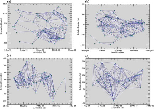
Table 2 reports the main parameters adopted to process the four SAR datasets with the SARscape® approach. To remove the topographic component of the phase, the Shuttle Radar Topography Mission (SRTM) DEM with a resolution of 1 arc second (approximately 30 m pixel size) was used. After the editing step in which the bad interferogram pairs are discarded for unwrapping and/or processing errors, a good amount of interferograms was still available. The edited CG plots for each dataset are reported in Figure 4.

Table 2. Main parameters and thresholds adopted in SARscape® for the SBAS processings.

Satellite	ERS-1/2	ENVISAT	TerraSAR-X	Sentinel-1A
Perpendicular thresh. (% of critical baseline)	50	45	35	45
Temporal thresh. (days)	900	730	190	150
Unwrapping thresh.	0.30	0.35	0.40	0.60
Multi-look Rg/Az	1/5	1/5	5/5	5/1
Resolution (m)	20	20	10	20
No. of generated interferograms	274	380	360	200

Figure 4. Interferogram pairs selected with SBAS after the editing session for (a) ERS-1/2, (b) ENVISAT, (c) TerraSAR-X, (d) Sentinel-1A.

The SUBSOFT processor, used to process the ENVISAT and TerraSAR-X data only, was implemented at the Remote Sensing Laboratory of the Universitat Politècnica de Catalunya and is based on the algorithms proposed by Mora, Mallorqui, and Broquetas (2003) and by Iglesias, Mallorqui, and Lopez-Dekker (2014). The algorithm scheme is made of three main steps: (a) generation of the best interferogram set; (b) selection of the pixels with reliable phase within the interferogram set; and (c) pixels phase analysis to calculate the deformation time series. For the pixel selection, the Temporal Sublook Spectral Coherence method, described previously, has been chosen. This method permits the selection of point-like scatterers by replacing the spatial average, which generates a degradation of the spatial resolution, with a temporal one. Specifically, the method is based on the analysis of their spectral properties along time. After the pixel selection, a Delaunay triangulation between the selected pixels is generated. Finally, the linear and nonlinear deformations are computed through a model of coherence estimation.

With the SUBSOFT processor is not possible to generate Single Look Complex (SLC) (Level 1 product) images directly from the raw data (Level 0 product), and of the 60 ENVISAT images, only 39 were provided by European Space Agency as SLC. For this reason, only a smaller number of ENVISAT images covering the period December 2005–September 2010 were processed to perform the cross-validation. For ENVISAT, the adopted processing parameters consist of a maximum spatial and temporal baseline, respectively, of 300 m and 246 days, a multi-look factor of 15 × 3 in range and azimuth, and an unwrapping threshold of 0.40. Considering these parameters, the obtained displacement standard deviation was 1.5 mm. In total, 80 interferograms were generated. The topographic component of the phase was removed using the ~30 m resolution SRTM DEM.

For the TerraSAR-X data processing, a maximum spatial baseline of 125 m and a maximum temporal baseline of 125 days have been used. Considering the adopted spatial baseline threshold, 11 images not respecting the constrain have been dropped. From the remaining 42 images, 220 interferograms have been selected. The applied multi-look factor is 3 × 3 in range and azimuth, and the coherence threshold is 0.4, which implies a phase standard deviation of 15°: the corresponding displacement standard deviation is about 1 mm. The topographic component of the phase was removed using the ~30 m resolution SRTM DEM.

3.2. Statistical analyses

Two statistical approaches were applied to the SBAS results in a Geographical Information System (GIS) in order to (a) identify the main areas affected by subsidence through the ground-motion areas detection and (b) comprehend the deformation mechanisms analyzing their relationships with the main triggering factors.

The ground-motion areas detection method proposed by Bonì, Pilla, and Meisina (2016) is addressed to simplify the analysis of very large point datasets resulting from A-DInSAR processing, using a fast and systematic procedure. The methodology allows us to identify areas that present significant movements, the ground-motion areas, considering specific patterns in the time series of each measured point. This method can be very useful to highlight areas with peculiar ground deformation behavior that may require more deep analyses. The applied procedure consists of two main steps: (1) the time series accuracy assessment is performed applying the approach proposed by Notti et al. (2015) in order to correct anomalous displacements affecting the time series in a certain date; and (2) different statistical tests are applied to find the spatiotemporal pattern of the Principal Components (PC) of the movement and the kinematic model of the measured points. In particular, the Principal Component Analysis was performed implementing a matrix organization location versus time (T-mode) to detect the PC of ground motion (Chaussard et al. 2014). The number of time-dependent components was detected for each dataset considering the change of slope in the Scree plot. Each component was represented by score maps as applied by others authors (Chaussard et al. 2014). More specifically, the PC scores obtained for each measured point represent the value of correlation with the trend of the PC in the whole dataset; the higher values correspond to higher correlation with the analyzed PC (Bonì, Pilla, and Meisina 2016). The software PSTime (Berti et al. 2013) was used to classify the time series into one of the three predefined target trends: uncorrelated, linear, and nonlinear (Berti et al. 2013). The approach is based on a sequence of statistical characterization tests that permit the automatic classification of each measured point. PSTime also detects the date (break date) where an abrupt slope change in the nonlinear time series is recorded. The evidence ratio of the break point (BICW) index (Berti et al. 2013) is also assigned to the nonlinear time series. The ground-motion areas were identified using a spatial cluster of the significant PC scores using a buffer zone of 50 m around each measured point. The PC score was used to find the spatial distribution of the ground-motion areas using the approach implemented by Meisina et al. (2008). The obtained kinematic model of the measured points was combined with the ground-motion areas to identify linear and nonlinear processes: values of BICW higher than 1.2 were selected to distinguish nonlinear time series from the linear ground-motion areas.

With the second statistical approach, the variance analysis is applied to the SBAS results, already imported in a GIS, to combine each measured point with the available ancillary data, evaluating the contribution to the subsidence of four main factors: geological setting, water extraction, gas extraction, and land-use change. In particular, the analyses are carried out considering the relationship between the measured displacement values and the lithologies in the study area, the position of the water pumping wells, the distance from the methane gas reservoirs and their production rates, the areas where land-use changes occurred. This method is based on the variances ratio and uses the distribution of Fisher–Snedecor (Fisher 1942; Snedecor and Cochran 1967).

4. Results and discussion

4.1. A-DInSAR SBAS results

The results obtained from the SBAS processing are reported as cumulated displacement maps projected to the vertical (Figure 5). In total, we detected 53,000 points with ERS-1/2, 71,200 with ENVISAT, 304,000 with TerraSAR-X and 100,000 with Sentinel-1A. The range of the detected velocities in the entire monitoring period (1992–2016) goes from −30 mm/year to +5 mm/year. Data coverage is good for all the datasets and is concentrated over the urbanized areas that present high coherence values. Strong subsidence mainly occurs along the coastal areas with higher values registered in the north and south. Most of the city center is stable, with displacement values in the range of ±5 mm for the entire period.

Figure 5. Vertical displacement maps obtained from the processing of (a) ERS-1/2 (1992–2000), (b) ENVISAT 2003–2010, (c) TerraSAR-X (2012–2014), and (d) Sentinel-1A (2014–2016) SAR images through SARscape®. The black dots, from P1 to P8, are the locations of the points considered for the time series analysis.

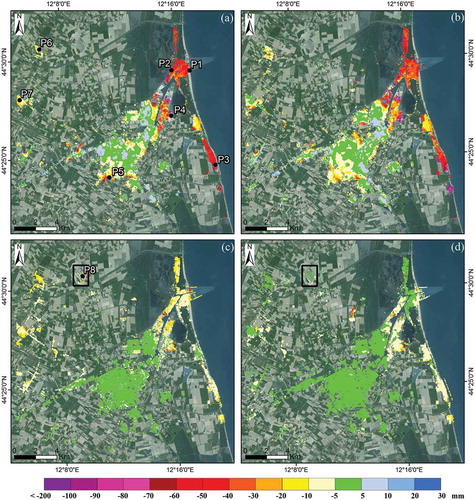
In Figure 5(c,d), it is possible to notice a subsiding area detected in the north part of the study area (black square). This area is a solar panel field of recent construction that was completed in early 2011 and expanded with two new small adjacent solar fields in early 2012. This area is clearly visible with both TerraSAR-X and Sentinel-1A datasets showing the capabilities of the latter in the monitoring of ground displacement even at local scale. The subsidence affecting this area is probably caused by the load produced by the panels structure itself over rural land. Here, the maximum displacement registered reached −21 mm during 2012–2014 and −11 mm in 2014–2016.

To better understand the displacement patterns in the study area, the time series of seven control points (Figure 5(a)) have been analyzed. The points were selected in the most critical areas, where the resulted subsidence values are high, or in areas that present anomalous displacement in respect to the surroundings (e.g. localized subsidence in a generally stable area). The analysis takes into account the average displacement values of all the points that are within a distance of 100 m from the selected points in order to minimize the effect of outliers. For each point, the time series are generated (Figure 6) considering as linear the displacement velocity in the temporal gaps between the different datasets: 28 months between ERS-1/2 and ENVISAT, 17 months between ENVISAT and TerraSAR-X, and 6 months between TerraSAR-X and Sentinel-1A.

Figure 6. Cumulated displacement time series for the eight selected points reported in Figure 5(a,c).

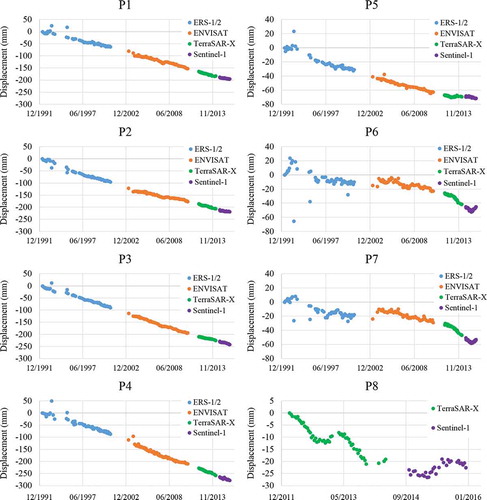
Considering the CG plot of Figure 4(a), the 57 images available for ERS-1/2 are not well distributed in time and present from 1992 to 1995 a large time gap of around 700 days that separates 12 images (left side) from the main cluster (right side). Since we needed to analyze the subsidence trends for the entire 1992–2000 period without losing any image, we adopted a temporal threshold of 900 days in order to connect all possible pairs. Unfortunately, the 700-day temporal baseline interferograms presented temporal decorrelation and consequent low coherence that reduced their quality. For this reason, during the 1992–1995 period, some phase unwrapping errors occurred and generated the anomalous displacement values that are visible in the time series of Figure 6. Taking into account the entire 1992–2016 period, the time series of the points located close to the coastline show an almost linear trend of deformation with low variation in the slope of the linear regression line. These points present the highest displacement values that were calculated as −250 mm at Lido Adriano (P3) and as −280 mm in the industrial area (P4). The time series obtained for the latter shows an almost constant velocity for the entire period. Along the coastline, the point P3 presents a linear subsidence trend until 2001 (−7 mm/year); the trend starts to increase from 2003 until the end of 2015 (−11 mm/year) and then it decreases again with values lower than the first period (−6 mm/year). On the contrary, 9 km to the north, the point located at Porto Corsini (P1) shows a constant increase of the displacement velocities from −7.8 mm/year (1992–2000) to around −9.3 mm/year (2014). The rates start to lower in 2014–2016 with −5 mm/year. The points less affected by subsidence are the ones located at Ravenna (P5) with around −70 mm of cumulated displacement, and to the west of the study area in the towns of Savarna and Mezzano (points P6 and P7, respectively). Here the maximum displacement reached −60 mm in both locations. Even if the two towns are located at a distance of 5 km, there is a strong correspondence in the displacement trend that is not linear but presents fluctuations in the entire period. The slope of the linear fitting line remains constant during 1992–2010 with a velocity of around −2 mm/year. The slope starts increasing from 2012 to 2013 and becomes steeper from April 2013 to June 2015, when the velocity reaches −9 mm/year. The time series of P8, located over the solar panel field, presents a clear seasonal trend during the period 2012–2016, detected by both TerraSAR-X and Sentinel-1A satellites.

4.2. Cross-validation with the CPT technique

In order to assess the reliability of the results obtained with SBAS, the ENVISAT and TerraSAR-X datasets have been reprocessed using the CPT technique and the outputs have been used for the cross-validation. The two approaches based on different phase quality estimation criteria can provide complementary information. In fact, the amplitude-based criterion generally provides high point density that can be used to carry out analyses at high resolution such as for the monitoring of buildings (Tomás et al. 2014). On the other hand, to monitor subsidence or volcanic activity over larger areas, the coherence-based processing is generally better suited. For this reason, a good match between the results obtained with the two techniques (cross-validation) can give a good indication of the processing quality and can be used as an effective validation method. As shown in other comparison experiments between A-DInSAR techniques (e.g. Herrera et al. 2009), in spite of their different pixel selection criterion based on the phase quality estimation, both approaches exhibit good performance in estimating deformations; their main difference consists of the operative resolution.

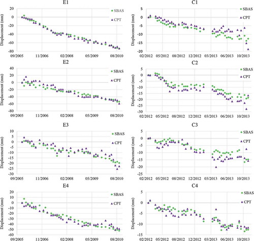
The ENVISAT and TerraSAR-X processing with CPT was carried out over a small area of 6 km × 3 km that covers the industrial area of Ravenna (Figure 1(b)), chosen because it is affected by very high rates of subsidence and presents high coherence values that permits to optimize the comparisons. The results, reported as vertical displacement map (Figure 7(c,d)), are in good agreement with the SBAS results obtained over the same area (Figure 7(a,b)). The lower number of points obtained with the CPT in respect to SBAS (369 versus 5896 for ENVISAT and 16,500 versus 28,700 for TerraSAR-X) is due to the more restrictive thresholds and higher multi-look factor adopted in the processing steps as described in Section 3.1. The time series of the four points selected for each dataset for the comparisons (Figure 8) show a good correspondence between CPT and SBAS in terms of mean velocity and displacement trends. It is possible to notice a shift in the calculated displacement of about 2–3 mm/year in each time series that is probably due to the different algorithm and methodology applied. This can be explained with the settings of the adopted processing parameters, such as coherence threshold and multi-look (described in Section 3.1), that implies different displacement standard deviations: for the TerraSAR-X data processing, the obtained standard deviation was 1.5 mm with SBAS and 1.0 mm with CPT, while for ENVISAT, it was 5.0 mm and 1.5 mm with SBAS and CPT, respectively. The comparison depicts the goodness of the results obtained with the SBAS technique.

Figure 7. Cumulated displacement maps over the industrial area of Ravenna used to cross-validate the results: (a) ENVISAT processed with SBAS. (b) TerraSAR-X processed with SBAS. (c) ENVISAT processed with CPT. (d) TerraSAR-X processed with CPT. The black dots, from E1 to E4 and from C1 to C4, are the locations of the points selected to perform the comparison between the time series obtained, respectively, from ENVISAT and TerraSAR-X.

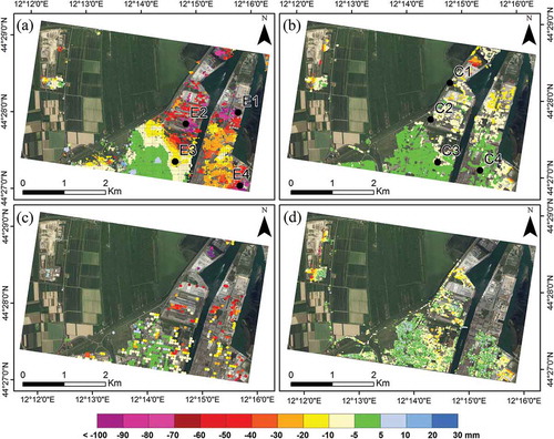
Figure 8. Time series of the control points selected in the industrial area of Ravenna obtained with SBAS and CPT. E1–E4: ENVISAT; C1–C4: TerraSAR-X.

4.3. Identification of ground-motion areas

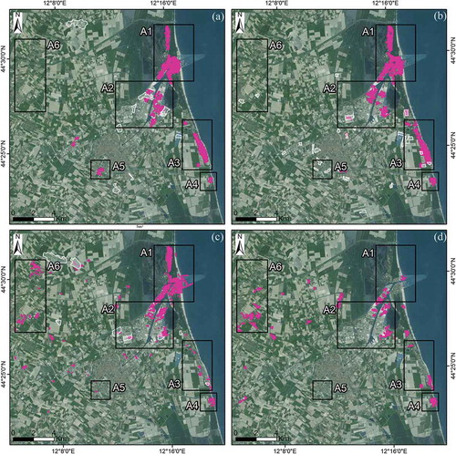
The ground-motion detection methodology was applied to the A-DInSAR results considering three main components of motion: PC1, which describes a movement away from the satellite (i.e. subsidence); PC2, which describes a movement toward the satellite (i.e. uplift); and PC3, which describes a seasonal component of motion. The results reveal that PC1 accounts for the 80–90% of the variance for all datasets while PC2 and PC3 explain the variance in a range from 1% to 10% of ENVISAT, TerraSAR-X, and Sentinel-1A results. Considering that PC1 better describes most of the components of motion in all datasets, the analyses were performed using only PC1. Figure 9 shows the spatial distribution of the ground-motion areas detected using PC1 of the four datasets. According to the methodology, six main subsiding areas have been identified: Porto Corsini (A1), the industrial area (A2), Lido Adriano (A3), Lido di Dante (A4), the southwest area of Ravenna (A5), and Savarna and Mezzano (A6).

Figure 9. In pink, the six ground-motion areas delimited by squares (A1: Porto Corsini; A2: Industrial Area; A3: Lido Adriano; A4: Lido di Dante; A5: South-west of Ravenna; A6: Savarna and Mezzano) detected using the PC1 main component of motion for (a) ERS-1/2, (b) ENVISAT, (c) TerraSAR-X, and (d) Sentinel-1A datasets. The white striped areas are the Corine Land Cover changes described in Section 4.4.

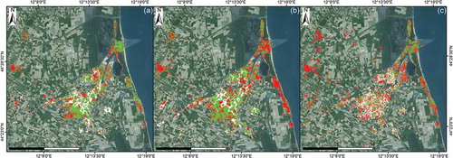
After selecting the measured points localized in the six ground-motion areas affected by subsidence, the average velocity and the standard deviation for each dataset have been calculated (Table 3). Regarding the kinematic model, the results (Figure 10) highlight that 40–50% of the points measured using ERS-1/2 and ENVISAT datasets is characterized by a linear trend, 30–40% show a nonlinear trend, and 20–30% show an uncorrelated trend. Most of the measured points (around 43%) resulting from the TerraSAR-X data processing show a nonlinear trend, while 30% is characterized by a linear trend and 27% by an uncorrelated trend. Unfortunately, the kinematic model analysis cannot be performed with the Sentinel-1A results, because the automatic procedure can work only with time series longer than 22 months.

Table 3. Average vertical velocity (Vvert) and standard deviation (Std) calculated in the six different ground-motion areas for each dataset.

Period		10 May 1992–13 December 2000	02 April 2003–22 September 2010	25 February 2012–05 April 2014	12 October 2014–11 January 2016
Dataset		ERS-1/2	ENVISAT	TerraSAR-X	Sentinel-1A
A1 (Porto Corsini)	Vvert (mm/year)	−7.23	−6.17	−7.91	−2.09
	Std (mm/year)	2.34	1.31	0.85	0.85
A2 (Industrial area)	Vvert (mm/year)	−6.37	−8.39	−10.05	−15.25
	Std (mm/year)	2.17	3.35	4.49	9.46
A3 (Lido Adriano)	Vvert (mm/year)	−6.83	−7.12	−7.07	−8.52
	Std (mm/year)	1.24	2.07	1.27	0.90
A4 (Lido di Dante)	Vvert (mm/year)	−7.94	−12.74	−7.45	−10.68
	Std (mm/year)	0.92	1.47	0.94	1.12
A5 (Southwest of Ravenna)	Vvert (mm/year)	−6.10	−5.23	−5.23	−2.72
	Std (mm/year)	2.27	0.87	0.94	0.43
A6 (Savarna and Mezzano)	Vvert (mm/year)	−3.70	−3.68	−10.11	−3.31
	Std (mm/year)	0.78	0.69	0.72	1.76

Figure 10. Points measured with (a) ERS-1/2, (b) ENVISAT, and (c) TerraSAR-X, classified by their kinematic model: linear trend in green, nonlinear trend in red, and uncorrelated trend in white.

4.4. Interpretation of ground-motion areas

Statistical analyses were used to interpret which are the main factors influencing the detected ground-motion areas. Unfortunately, the restricted availability of ancillary data limited the number of the possible factors to analyze. Anyway, the results obtained so far are in accordance with the main conclusions of the scientific literature (e.g. Teatini et al. 2005).

A first analysis was carried out to evaluate the influence that the geology has on the deformation values, associating the available geological information (Figure 1(c)) to each point measured with SBAS. For all the four A-DInSAR processings, the test has shown a high influence of the geology on the measured deformation with values increasing toward the coastline. Specifically, bigger deformations occur over the fluvial sands lithology with an average value of −27.4 ± 26.5 mm for 1992–2000, −26.5 ± 27.8 mm for 2003–2010, −7.8 ± 6.9 mm for 2012–2014, and −4.2 ± 4.6 mm for 2014–2016. Small deformations are observed on the lithified marine dune with an average of −1.1 ± 9.5 mm for 1992–2000, −3.2 ± 12.4 mm for 2003–2010, −1.5 ± 5.3 mm for 2012–2014, and −2.6 ± 6.1 mm for 2014–2016.

A second analysis was applied to assess the relationship between the water wells, classified by type of use (agricultural, civil, and livestock) and the subsidence velocity. Unfortunately, no data about the pumping rates for each well is available, so the analysis is based only on their location. A fishnet with cell size of 1 km × 1 km has been created and the average velocity for each cell has been computed (Figure 11).

Figure 11. Average vertical velocities of deformation computed with a fishnet of 1 km × 1 km for each dataset. The location of the three categories of water wells and the extension of the methane gas fields are superimposed to the fishnet used in the statistical analyses.

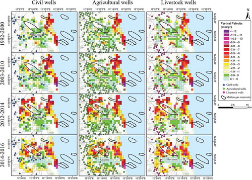
The test does not show significant influence of the wells location on the subsidence velocities. A better correspondence was found only for the agricultural wells located in the northwestern part of the study area where agricultural activities continue to be prevalent.

In order to analyze the relationship between deformation and the gas extractions, the spatial correlation with the methane gas field, the distance–velocity plots along with the gas production have been taken into account. We focused on Angela-Angelina and on Porto Corsini Terra gas fields.

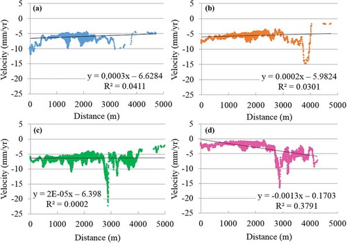
Regarding Angela-Angelina (Figure 12), the average velocity values of the points closer to the reservoir are, respectively, of −1.1 ± 1.1 mm/year, −11.1 ± 1.3 mm/year, −6.9 ± 1.3 mm/year, and −7.8 ± 1.1 mm/year for ERS-1/2, ENVISAT, TerraSAR-X, and Sentinel-1A. The intercepts of the diagrams are of −9 mm/year, −11 mm/year, −6 mm/year, and −8 mm/year for the four results.

Figure 12. Velocity–distance plots for the Angela-Angelina gas field. (a) ERS-1/2, (b) ENVISAT, (c) TerraSAR-X, (d) Sentinel-1A.

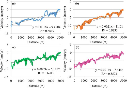
It is possible to notice a general decrease of the measured deformations for increasing distances from the reservoir. Considering the average velocities of displacement in A3 and A4, there is an increase in the subsidence rates in the period 2003–2010 in respect to 1992–2000 and in the period 2014–2016 in respect to 2012–2014. The average velocity is higher in area A4 than in area A3. Considering the gas production activity in 1990–2016 (Figure 2), there is a quite good correlation with the measured deformations. The increase of the average velocity, detected using ENVISAT, can be related to the increase of the methane gas extractions in 1998 (1748 × 10⁶ Sm³). In 2012–2014, the decrease of the average velocity can be correlated with a decrease in the methane gas production from an annual average of 734 × 10⁶ Sm³ to 377 × 10⁶ Sm³. Conversely, the increase average velocity detected in the period 2014–2016 in both A3 and A4 is not correlated with the methane gas production.

Even for the Porto Corsini Terra gas field, the analysis shows a general decrease of the deformations with increasing distance from the gas reservoir, especially in the northern side of the gas field (Figure 13) within a distance lower than 1 km.

Figure 13. Velocity–distance plots for the Porto Corsini Terra gas field. (a) ERS-1/2, (b) ENVISAT, (c) TerraSAR-X, (d) Sentinel-1A.

The area closest to Porto Corsini Terra, A1, presents an increase of the average velocity from 2012–2014 to 2003–2010, while in 2014–2016, the velocity rapidly decreased until −2.09 mm/year. The high average velocities found in 1992–2014 may correspond to the combined effects of the extraction activities taking place in the two gas reservoirs close to the area: Porto Corsini Terra and Porto Corsini Mare Ovest (Figure 1(b)). Despite the low production rates of the first, the proximity to A1 (around 1.5 km) may strongly influence the subsidence in the area. The maximum production in 2003 of 42.6 × 10⁶ Sm³ drastically lowered in the next years until ending in 2014. The Porto Corsini Mare Ovest reservoir is located around 5 km west of A1 and had a very high productivity in 2004–2008 with more than 260 × 10⁶ Sm³. In this case, the production ended in 2016. The decrease in the average velocity in 2014–2016 (−2.09 mm/year) reflects the reduced methane gas production in the two gas fields in those years.

4.5 Land-use change

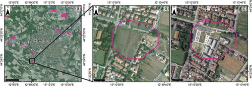
The contribution that land-use changes may have on the detected displacement rates was evaluated by overlapping the six ground-motion areas with the CORINE Land Cover (CLC) inventory (EEA 2007) corresponding to the period covered by each dataset (Figure 9). The ground-motion areas extracted from the ERS-1/2 results were compared with the 1990–2000 CLC changes. In A2, part of the subsidence occurs in areas which land-use changed from salt marshes and nonirrigated arable land to industrial/commercial unit. The displacement observed with the ENVISAT data matches with the 2000–2006 CLC changes. A correlation between land use changes from arable land to industrial/commercial unit was detected in A3. Also in A2, the motion areas partly match with land use that changed from arable land to construction unit. Therefore, in A2, part of the subsidence seems to be correlated to the sediments compaction caused by the load produced by the new constructions. Comparing the 2012–2013 CLC changes with the TerraSAR-X results, the same correlation was observed in a small area of A3 where the same land-use change occurred. The ground-motion area detected in A5 highlights a decrease of the average velocity from −6.10 mm/year (1992–2000) to −2.72 mm/year (2014–2016). Unfortunately, no CLC changes are available for this area after 2006, but the comparison of the Google™ earth DigitalGlobe historic images 17 October 2009–7 June 2014 (Figure 14) shows new constructions in areas used as arable land. This may explain the relatively high average velocity (−5.23 mm/year) registered in the area during 2012–2014. The ground-motion area detected at Savarna and Mezzano (A6) is characterized by a high increase of the average velocity from around −3.7 mm/year of 1992–2010 to −10.11 mm/year of 2012–2014; it follows a rapid decrease in 2014–2016 with −3.3 mm/year. In this case, a strong correlation between the CLC change and subsidence did not result from the analysis. Only in few small areas of A6, the recent constructions that are visible comparing the Google™ earth DigitalGlobe historic images from 2006 to 2015 may explain local accelerations in the subsidence rates.

Figure 14. (a) Ground-motion areas detected for the TerraSAR-X results. In (b) and (c), the comparison between the Google™ earth DigitalGlobe images 17 October 2009 and 7 June 2014 showing new urban development in A5.

5. Conclusions

The land subsidence affecting the city of Ravenna and its surrounding was measured using 25 years (1992–2016) of SAR data acquired by ERS-1/2, ENVISAT, TerraSAR-X, and Sentinel-1A satellites. The A-DInSAR results reported as displacement maps projected to the vertical direction show subsidence up to −35 mm/year affecting mainly the coastline and the industrial area of Ravenna. The analysis of the displacement time series was carried out over seven selected points that present mostly a linear trend. The points located along the coastline and in the industrial area present the highest displacement values in the 1992–2016 period, which was calculated as −250 mm and −280 mm, respectively. Statistical analyses were applied in order to better understand the behavior of the displacement over time and to assess the role of the main factors that control the subsidence. The analyses revealed that the main driving factor of the subsidence along the coastline can be related to the exploitation of the on and offshore methane gas fields. There is no evident relationship between the water extraction and the detected displacements, while the correlation with the geology appears to be strong. One more factor considered was the land-use change that in many restricted areas explains the high rates of subsidence caused by the sediments consolidation under the loading of newly developed residential or industrial areas.

The results obtained with SBAS from the ENVISAT and TerraSAR-X images were cross-validated through the comparison with the CPT processing over the industrial area of Ravenna. The analysis of the time series of four control points showed that the displacement trends obtained with both techniques were very similar, confirming the validity of the SBAS results.

The study shows the benefits of a long-term monitoring activity performed using A-DInSAR techniques thanks to which it is possible to monitor very large areas with metric resolution and millimeter accuracy. The availability of the new Sentinel-1A data, in particular, further improves the monitoring activity giving up to date information on the subsidence behavior. The short revisiting time of 12 days of Sentinel-1A, not only permits to obtain better data coverage with increased points density, but also enhance the displacement time series analysis that now are sensible to seasonal trends, rainy periods, or thermic variations. Furthermore, the launch in April 2016 of the twin satellite Sentinel-1B will reduce the revisiting interval to 6 days allowing us to perform near-real time and continuous monitoring activities.

Anyway, A-DInSAR results must always be integrated with other analyses in order to fully exploit their potential. In our case, the statistical analyses proved to be reliable tools that, applied to the deformation and velocity maps obtained with SBAS, allowed us to better understand the subsidence trends, its main driving factors, and the relationship with the exploitation of the underground resources in the area. Future work will regard the extension of the monitoring activity with the latest Sentinel-1A and -1B images along with the integration of other ancillary data to improve the statistical analyses.

Acknowledgments

ERS-1/2 and ENVISAT images are provided by the European Space Agency (ESA) through the project C1P.14280. The TerraSAR-X images are provided by the German Space Agency (DLR) through the proposals GEO2478 and GEO3016. The Sentinel-1A and Sentinel-2 images are freely available from the ESA’s Sentinel DataHub (https://scihub.copernicus.eu). Authors would like to thank Prof. J.J. Mallorquì (Remote Sensing Laboratory of the Universitat Politècnica de Catalunya of Barcelona) for providing the SUBSOFT processor software. Authors would like to thank also the three anonymous reviewers for their careful reading of this manuscript and their insightful comments and suggestions.

Disclosure statement

No potential conflict of interest was reported by the authors.

References

- Amorosi, A. 1999. “Sedimentary Response To Late Quaternary Sea-level Changes In The Romagna Coastal Plain (Northern Italy).” Sedimentology 46: 99–121.
- ARPA (Regional Agency for the Environmental Protection) Emilia-Romagna and Regione Emilia-Romagna. 2010. “Applicazione della modellistica matematica di simulazione. Fase II: analisi della subsidenza nelle zone costiere.” Technical Report. Bologna, Italy. Accessed 12 June 2016. http://www.ARPA.emr.it/cms3/documenti/subsidenza/Relazione_FaseII.pdf
- Berardino, P., G. Fornaro, R. Lanari, and E. Sansosti. 2002. “A New Algorithm for Surface Deformation Monitoring Based on Small Baseline Differential SAR Interferograms.” IEEE Transactions on Geoscience and Remote Sensing 40: 2375–2383. doi:10.1109/TGRS.2002.803792.
- Berti, M., A. Corsini, S. Franceschini, and J. P. Iannacone. 2013. “Automated Classification of Persistent Scatterers Interferometry Time Series.” Natural Hazards and Earth System Sciences 13: 1945–1958. doi:10.5194/nhess-13-1945-2013.
- Bertoni, W., G. Brighetti, G. Gambolati, G. Ricceri, and F. Vuillermin. 1995. “Land Subsidence Due to Gas Production in the On- and Off-Shore Natural Gas Fields of the Ravenna Area, Italy”. In Land Subsidence, Proceedings of the Fifth International Symposium on Land Subsidence, The Hague, IAHS 234.
- Blanco, P., J. J. Mallorquí, S. Duque, and D. Navarrete. 2006. “Advances on Dinsar with ERS and ENVISAT Data Using the Coherent Pixels Technique (CPT).” Proceedings of IEEE International Geoscience and Remote Sensing Symposium 4: 1898–1901.
- Bonì, R., G. Pilla, and C. Meisina. 2016. “Methodology for Detection and Interpretation of Ground Motion Areas with the A-Dinsar Time Series Analysis.” Remote Sensing 8 (8): 686. doi:10.3390/rs8080686.
- Carbognin, L., and L. Tosi. 2002. “Interaction between Climate Changes, Eustacy and Land Subsidence in the North Adriatic Region, Italy.” Marine Ecology 23 (1): 38–50. doi:10.1111/j.1439-0485.2002.tb00006.x.
- Carminati, E., G. Martinelli, and P. Severi. 2003. “Influence of Glacial Cycles and Tectonics on Natural Subsidence in the Po Plain (Northern Italy): Insights from 14C Ages.” Geochemistry Geophysics Geosystems Journal 4: 1082–1096.
- Cascini, L., G. Fornaro, and D. Peduto. 2010. “Advanced Low- and Full-Resolution Dinsar Map Generation for Slow-Moving Landslide Analysis at Different Scales.” Engineering Geology 112: 29–42. doi:10.1016/j.enggeo.2010.01.003.
- Chaussard, E., R. Bürgmann, M. Shirzaei, E. J. Fielding, and B. Baker. 2014. “Predictability of Hydraulic Head Changes and Characterization of Aquifer‐System and Fault Properties from Insar‐Derived Ground Deformation.” Journal of Geophysical Research: Solid Earth 119 (8): 6572–6590.
- Chini, M., M. Albano, M. Saroli, L. Pulvirenti, M. Moro, C. Bignami, E. Falcucci, et al. 2016. “Coseismic Liquefaction Phenomenon Analysis by Cosmo-Skymed: 2012 Emilia (Italy) Earthquake.” International Journal of Applied Earth Observation and Geoinformation 39: 65–78. doi:10.1016/j.jag.2015.02.008.
- Costantini, M. 1998. “A Novel Phase Unwrapping Method Based on Network Programming.” IEEE Transactions on Geoscience and Remote Sensing 36 (3): 813–821. doi:10.1109/36.673674.
- Costantini, M., and P. A. Rosen. 1999. “A Generalized Phase Unwrapping Approach for Sparse Data”. In Proceedings of IEEE International Geoscience and Remote Sensing Symposium, Vol. 1, Hamburg, June 28- June-2, 267–269.
- Di Martire, D., A. Novellino, M. Ramondini, and D. Calcaterra. 2016. “A-Differential Synthetic Aperture Radar Interferometry Analysis of a Deep Seated Gravitational Slope Deformation Occurring at Bisaccia (Italy).” Science of the Total Environment 550: 556–573. doi:10.1016/j.scitotenv.2016.01.102.
- EEA (European Environmental Agency). 2007. “Technical Report.” Accessed 12 August 2016. http://land.copernicus.eu/user-corner/technical-library/CLC2006_technical_guidelines.pdf
- ENI (National Hydrocarbons Authority) S.p.A–AGIP and ARPA Emilia-Romagna. 2003. “Studio della Subsidenza Antropica generata dall’estrazione di acqua di falda lungo la costiera emiliano-romagnola.” Technical report. Accessed 13 June 2016. http://www.ARPAe.it/cms3/documenti/subsidenza/Relfin_Agip_2003_rid.pdf
- Ferretti, A., C. Prati, and F. Rocca. 2000. “Nonlinear Subsidence Rate Estimation Using Permanent Scatterers in Differential SAR Interferometry.” IEEE Transactions on Geoscience and Remote Sensing 38: 2202–2212. doi:10.1109/36.868878.
- Ferretti, A., C. Prati, and F. Rocca. 2001. “Permanent Scatterers in SAR Interferometry.” IEEE Transactions on Geoscience and Remote Sensing 39 (1): 8–20. doi:10.1109/36.898661.
- Fisher, R. A. 1942. The Design of Experiments. 3rd ed. Edinburgh: Oliver & Boyd.
- Gabriel, K., R. M. Goldstein, and H. A. Zebker. 1989. “Mapping Small Elevation Changes over Large Areas: Differential Radar Interferometry.” Journal of Geophysical Research 94: 9183. doi:10.1029/JB094iB07p09183.
- Gambolati, G., G. Ricceri, W. Bertoni, G. Brighenti, and E. Vuillermin. 1991. “Mathematical Simulation of the Subsidence of Ravenna.” Water Resources Research 27: 2899–2918. doi:10.1029/91WR01567.
- Gambolati, G., and P. Teatini. 1998. “Numerical Analysis of Land Subsidence Due to Natural Compaction of the Upper Adriatic Sea Basin.” In CENAS, Coastline evolution of the upper Adriatic Sea due to sea level rise and natural and anthropogenic land subsidence, Kluwer Academic Publishing, Water Science & Technology Library, 28: 103–131.
- Gambolati, G., P. Teatini, L. Tomasi, and M. Gonella. 1999. “Coastline Regression of the Romagna Region, Italy, Due to Natural and Anthropogenic Land Subsidence and Sea Level Rise.” Water Resources Research 35 (1): 163–184. doi:10.1029/1998WR900031.
- Ghielmi, M., M. Minervini, C. Nini, S. Rogledi, M. Rossi, and A. Vignolo. 2010. “Sedimentary and Tectonic Evolution in the Eastern Po-Plain and Northern Adriatic Sea Area from Messinian to Middle Pleistocene (Italy).” Rendiconti Lincei 21 (1): 131–166. doi:10.1007/s12210-010-0101-5.
- Goldstein, R. M., and C. L. Werner. 1998. “Radar Interferogram Filtering for Geophysical Applications.” Geophysical Research Letters 25 (21): 4035–4038. doi:10.1029/1998GL900033.
- Herrera, G., R. Tomás, J. M. Lopez-Sanchez, J. Delgado, F. Vicente, J. Mulas, G. Cooksley, et al. 2009. “Validation and Comparison of Advanced Differential Interferometry Techniques: Murcia Metropolitan Area Case Study.” ISPRS Journal of Photogrammetry and Remote Sensing 64: 501–512. doi:10.1016/j.isprsjprs.2008.09.008.
- Iglesias, R., J. J. Mallorqui, and P. Lopez-Dekker. 2014. “Dinsar Pixel Selection Based on Sublook Spectral Correlation along Time.” IEEE Transactions on Geoscience and Remote Sensing 52 (7): 3788–3799. doi:10.1109/TGRS.2013.2276023.
- Lanari, R., O. Mora, M. Manunta, J. J. Mallorqui, P. Berardino, and E. Sansosti. 2004. “A Small-Baseline Approach for Investigating Deformations on Full-Resolution Differential SAR Interferograms.” IEEE Transactions on Geoscience and Remote Sensing 42 (7): 1377–1386. doi:10.1109/TGRS.2004.828196.
- Massonnet, D., P. Briole, and A. Arnaud. 1995. “Deflation of Mount Etna Monitored by Spaceborne Radar Interferometry.” Nature 375: 567–570. doi:10.1038/375567a0.
- Massonnet, D., M. Rossi, C. Carmona, F. Adragna, G. Peltzer, K. Feigl, and T. Rabaute. 1993. “The Displacement Field of the Landers Earthquake Mapped by Radar Interferometry.” Nature 364: 138–142. doi:10.1038/364138a0.
- Meisina, C., F. Zucca, D. Notti, A. Colombo, A. Cucchi, G. Savio, C. Giannico, and M. Bianchi. 2008. “Geological Interpretation of Psinsar Data at Regional Scale.” Sensors 8 (11): 7469–7492. doi:10.3390/s8117469.
- Meyer, F. J., D. B. McAlpin, W. Gong, O. Ajadi, S. Arko, P. W. Webley, and J. Dehn. 2015. “Integrating SAR and Derived Products into Operational Volcano Monitoring and Decision Support Systems.” ISPRS Journal of Photogrammetry and Remote Sensing 100: 106–117. doi:10.1016/j.isprsjprs.2014.05.009.
- Mora, O., J. J. Mallorqui, and A. Broquetas. 2003. “Linear and Non-Linear Terrain Deformation Maps from a Reduced Set of Interferometric SAR Images.” IEEE Transactions on Geoscience and Remote Sensing 41: 2243–2253. doi:10.1109/TGRS.2003.814657.
- Notti, D., F. Calò, F. Cigna, M. Manunta, G. Herrera, M. Berti, C. Meisina, D. Tapete, and F. Zucca. 2015. “A User-Oriented Methodology for Dinsar Time Series Analysis and Interpretation: Landslides and Subsidence Case Studies.” Pure and Applied Geophysics 172 (11): 3081–3105. doi:10.1007/s00024-015-1071-4.
- Snedecor, G. W., and W. G. Cochran. 1967. Statistical Methods. 6th ed. Ames: Iowa State University Press.
- Soergel, U., ed. 2010. Radar Remote Sensing of Urban Areas. Vol. 15. Dordrecht: Springer.
- Teatini, P., M. Ferronato, G. Gambolati, W. Bertoni, and M. Gonella. 2005. “A Century of Land Subsidence in Ravenna, Italy.” Environmental Geology 47: 831–846. doi:10.1007/s00254-004-1215-9.
- Tessitore, S., J. A. Fernández-Merodo, G. Herrera, R. Tomás, M. Ramondini, M. Sanabria, J. Duro, J. Mulas, and D. Calcaterra. 2016. “Comparison of Water-Level, Extensometric, Dinsar and Simulation Data for Quantification of Subsidence in Murcia City (SE Spain).” Hydrogeology Journal 24 (3): 727–747. doi:10.1007/s10040-015-1349-8.
- Tomás, R., Y. Márquez, J. M. Lopez-Sanchez, J. Delgado, P. Blanco, J. J. Mallorquí, M. Martínez, G. Herrera, and J. Mulas. 2005. “Mapping Ground Subsidence Induced by Aquifer Overexploitation Using Advanced Differential SAR Interferometry: Vega Media of the Segura River (SE Spain) Case Study.” Remote Sensing of Environment 98 (2–3): 269–283. doi:10.1016/j.rse.2005.08.003.
- Tomás, R., R. Romero, J. Mulas, J. J. Marturià, J. J. Mallorquí, J. M. Lopez-Sanchez, G. Herrera, et al. 2014. “Radar Interferometry Techniques for the Study of Ground Subsidence Phenomena: A Review of Practical Issues through Cases in Spain.” Environmental Earth Sciences 71: 163–181. doi:10.1007/s12665-013-2422-z.