Biomass estimation of Sonneratia caseolaris (l.) Engler at a coastal area of Hai Phong city (Vietnam) using ALOS-2 PALSAR imagery and GIS-based multi-layer perceptron neural networks

Abstract

This study tested the use of machine learning techniques for the estimation of above-ground biomass (AGB) of Sonneratia caseolaris in a coastal area of Hai Phong city, Vietnam. We employed a GIS database and multi-layer perceptron neural networks (MLPNN) to build and verify an AGB model, drawing upon data from a survey of 1508 mangrove trees in 18 sampling plots and ALOS-2 PALSAR imagery. We assessed the model’s performance using root-mean-square error, mean absolute error, coefficient of determination (R²), and leave-one-out cross-validation. We also compared the model’s usability with four machine learning techniques: support vector regression, radial basis function neural networks, Gaussian process, and random forest. The MLPNN model performed well and outperformed the machine learning techniques. The MLPNN model-estimated AGB ranged between 2.78 and 298.95 Mg ha⁻¹ (average = 55.8 Mg ha⁻¹); below-ground biomass ranged between 4.06 and 436.47 Mg ha⁻¹ (average = 81.47 Mg ha⁻¹), and total carbon stock ranged between 3.22 and 345.65 Mg C ha⁻¹ (average = 64.52 Mg C ha⁻¹). We conclude that ALOS-2 PALSAR data can be accurately used with MLPNN models for estimating mangrove forest biomass in tropical areas.

Keywords:

• multi-layer perceptron neural networks
• ALOS-2 PALSAR
• biomass
• Hai Phong
• Sonneratia caseolaris

1. Introduction

The mangrove forest biome, commonly referred to as “mangroves” collectively, is the most important ecosystem within coastal inter-tidal zones in many tropical and semi-tropical regions. It plays a vital role in reducing damage from tsunamis (Danielsen et al. 2005), protecting land from erosion, and mitigating the effects of typhoons (Mazda et al. 1997). In addition, this ecosystem can act as a highly efficient carbon sink in the tropics (Donato et al. 2011), because mangroves can sequester carbon in both above and below-ground biomass as well as within sediment (Kauffman et al. 2014).

Despite the large carbon storage potential in mangrove biomass and soils, mangroves are under serious threat from high population growth, aquaculture expansion, timber harvesting, and other human activities (Duke et al. 2007). In Southeast Asia, mangroves have declined markedly suffering from the greatest loss of 1.9 million hectares (FAO 2007). Vietnam has experienced severe mangrove loss over the past 50 years (Tuan et al. 2003): on the northern coast in particular, mangrove area decreased by 17,094 ha from 1964 to 1997, largely due to over-expansion of shrimp farming (Tien Dat and Yoshino 2016).

Numerous studies have estimated mangrove biomass during the past 30 years (Tamai et al. 1986; Clough and Scott 1989; Jin-Eong, Khoon, and Clough 1995; Clough, Dixon, and Dalhaus 1997; Komiyama, Ong, and Poungparn 2008). Several studies established allometric equations to estimate the above-ground biomass (AGB) from in situ measurements (Chave et al. 2005), as well as forest inventory from biophysical parameters of mangrove trees such as stem weight, tree height and diameter at breast height (DBH) (Komiyama et al. 2002; Komiyama, Poungparn, and Kato 2005). The computational methods involved have included regression models (Ross et al. 2001; Chave et al. 2005) and machine learning (Jachowski et al. 2013). However, these studies were influenced by site selection biases and other factors such as tidal inundation (Ellison 2002; Alongi 2002). Current methods used can be time consuming, and costly, particularly in areas of dense mangrove forests, resulting in a lack of up-to-date information on spatial distribution of biomass and carbon stock. Thus, it is necessary to develop accurate and low-cost models to estimate mangrove biomass in order to support coastal zone management programs.

A variety of remote-sensing data have been widely used for mapping and monitoring mangrove forests including optical imagery (Long and Skewes 1996; Pasqualini et al. 1999; Conchedda, Durieux, and Mayaux 2008; Nandy and Kushwaha 2011; Long and Giri 2011) and synthetic aperture radar (SAR) data (Lucas et al. 2007; Tien Dat and Yoshino 2016). SAR sensors have been largely found to be more effective in monitoring mangrove dynamics as they can penetrate clouds, a common occurrence in the tropics (Lu 2006). Estimation of mangrove forests AGB is most accurate when conducted at the individual species level (Zhu et al. 2015). However, estimation of AGB using remote-sensing data for specific mangrove species, that is, Sonneratia caseolaris, has rarely been conducted. Thus, this study attempted to estimate the biomass and carbon stock of S. caseolaris (a dominant mangrove species in the study area) using ALOS-2 PALSAR imagery.

Biomass and carbon stock estimation of mangrove forests in Vietnam is still limited. Existing studies are restricted to specific regions, such as Ca Mau Peninsula in the south (Nguyen-Thanh et al. 2015) and Hai Phong, Quang Ninh in the North (Dat and Yoshino 2011; Tien Dat and Yoshino 2012). Several studies have attempted to estimate the biomass and carbon stock of mangrove plantation in the northern coast of Vietnam (Nguyen et al. 2004), in Quang Ninh province in the north, in Ca Mau and Kien Giang in the South (Vu, Takeuchi, and Van 2014), and in the Mekong Delta region (Nam et al. 2016). However, the spatial distribution of mangrove forest biomass and carbon stock in Vietnam is limited and not well documented. Thus, there is a need to quantify and assess these variables using a practical and cost-effective approach.

Recently introduced machine learning algorithms have been shown to be effective for modeling mangrove biomass and species distribution using remote-sensing data (Wang, Silván-Cárdenas, and Sousa 2008; Heumann 2011). However, there are several difficulties involved in implementing machine learning algorithms as long as traditional modeling techniques. The recent development of open-source software tools such as WEKA and Python has led to the wide use of machine learning (Hall et al. 2009; Pedregosa et al. 2011). Machine learning has become more common for the estimation of mangrove forest biomass due to its potential to produce better models than traditional modeling methods. Therefore, the investigation of machine learning algorithms for the estimation of mangrove forest biomass is highly necessary to support monitoring, reporting, and verification (MRV) work as part of the United Nations’ Reducing Emission from Deforestation and Forest Degradation (REDD+) program in developing countries.

Our study developed a prediction model using SAR remote-sensing imagery and multi-layer perceptron neural networks (MLPNNs) to estimate the biomass of a high-density mangrove species in the coastal area of Hai Phong city, Vietnam. According to current literature, this is the first time an estimation of AGB for S. caseolaris has been carried out in this area. Our work will allow further investigation into the functional condition of mangrove ecosystems in the study area and may help elucidate the spatial distribution patterns of biomass in tropical and sub-tropical climates. Our results also promote the implementation of REDD+ and payment for ecosystem services (PES) strategies by providing practical tools for developing regional and national blue carbon trading markets and guiding mangrove management and conservation.

Among various machine learning methods, artificial neural networks (ANNs) have great potential for nonlinear mapping, adaptive learning, and forecasting environmental problems, because they require no statistical assumptions on data distribution and have performed well in recent studies (Valipour, Banihabib, and Behbahani 2013; Valipour 2016). Many studies have used ANNs in modeling nonlinear relationship problems such as drought (Valipour 2016), surface irrigation systems (Valipour 2012; Valipour, Sefidkouhi, and Eslamian 2015; Mahdizadeh Khasraghi, Sefidkouhi, and Valipour 2015), and shallow landslide hazards (Tien Bui et al. 2016). However, ANNs have seldom been utilized for estimating mangrove forest biomass. More importantly, the ability of available machine learning techniques to estimate mangrove AGB has not been quantitatively assessed.

This study used ALOS-2 PALSAR data to investigate the applicability of MLPNNs for estimating the AGB of S. caseolaris in a coastal area of Hai Phong city, Vietnam. We also compared the MLPNNs’ performance with other machine learning techniques. Our results demonstrate that the use of ALOS-2 PALSAR imagery and MLPNNs for estimating mangrove forest biomass has the potential to support improved coastal conservation and management. We note that the data visualization and processing were carried out using ENVI 5.2 and ArcGIS 10.2 software, while the modeling process was conducted using Weka 3.7 software.

2. Study area and data

2.1 Description of study area

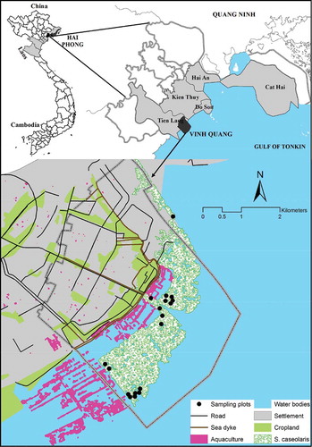
We conducted this study in the mangrove forests of Vinh Quang village, which belongs to the Tien Lang district of Hai Phong city (Figure 1). The coastline in this part of northern Vietnam consists of high tidal mudflats formed by a large quantity of alluvial sediment from the Red River. This area is vulnerable to rising sea levels and tropical storms, which often take place during the wet season from May to October (Hong, San, and Dao 1998). Part of the coastline is protected by the dominant mangrove species S. caseolaris (Tien Dat and Yoshino 2012; Tien Dat and Yoshino 2016), which plays an important role in wave reduction (Mazda et al. 2006) and contributes to the socioeconomic lives of local residents by providing forest products (Hong and San 1993).

Figure 1. Map of the study area at Vinh Quang coast, Tien Lang district, Hai Phong city. For full color versions of the figures in this paper, please see the online version.

2.2 Data collection and processing

2.2.1 SAR image collection and processing

We used ALOS-2 PALSAR satellite imagery (level 2.1, in high-sensitive polarimetric mode), acquired from the Remote Sensing Technology Centre (RESTEC) of Japan to estimate the biomass of S. caseolaris (Table 1).

Table 1. Acquired satellite remote-sensing data.

Satellite sensor	Date of acquisition	Level of process	Pixel spacing	Polarizations
ALOS-2 PALSAR	2015/7/31	2.1	6.25 m	L band (HH, HV)

Source: JAXA, Japan.

The digital number (DN) was converted to normalized radar sigma-zero using Equation (1):

(1)

where σ⁰ is the backscattering coefficient, DN is the digital number of the amplitude image, CF is the calibration factor, which is equal to −83 dB for both HH and HV polarizations (JAXA 2014). The CF used to process ALOS-2 PALSAR is similar to ALOS PALSAR (Shimada et al. 2009).

The DN of each pixel was transformed into backscattering sigma naught (σ⁰) in decibel (dB) after applying Forst filters with moving windows of 5 × 5 in order to reduce speckle noise of SAR data (De Leeuw and De Carvalho 2009). In order to minimize effects from tidal height, we also carefully took the time to conduct field work into consideration (Darmawan et al. 2015).

We employed ENVI 5.2 software for SAR imagery processing and S. caseolaris identification, as illustrated in Figure 2.

Figure 2. Flowchart used to identify S. caseolaris using ALOS-2 PALSAR imagery.

2.2.2 Field data collection

We conducted field survey measurements along the Vinh Quang coast in July 2015 with help and permission from local authorities. We selected plots using a stratified random sampling method in which strata were determined based on a pre-survey involving local people to ensure the range of biomass values would be valid for the entire mangrove forest. A total of eighteen sampling plots were measured for specific biophysical parameters such as diameter at breast height (DBH), tree height, and tree density. In addition, interviews with village heads, chairmen of farmer’s associations, and women’s reunions were conducted to understand the history of mangrove plantation programs in the area.

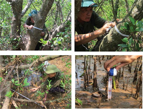
We also measured the height of S. caseolaris pneumatophores by establishing 1 × 1 m sub-plots to measure their maximum and minimum height along with a root count. The four corners of each sampling plot were established in the field using a Garmin Global Positioning Systems (GPS) eTrex Legend HCx unit, with a plot size of 30 × 30 m to access the ALOS-2 PALSAR pixel size of 6.25 × 6.25 m (Figure 3). The field data were divided into two sets: the first was used to estimate mangrove AGB using machine learning algorithm models, while the second was used for model validation. Photos and locations of the plots were also recorded using GPS during the field survey. Figure 3 shows the techniques used to measure biophysical parameters of S. caseolaris and their roots in a sub-plot.

Figure 3. Measurement biophysical parameters of S. caseolaris and their roots.

The above-ground biomass (AGB) and below-ground biomass (BGB) of S. caseolaris were calculated using the allometric Equations (2) and (3) (Komiyama, Poungparn, and Kato 2005):

(2)

(3)

where AGB and BGB indicate tree weight (kg), D is the diameter at breast height (DBH) (cm), H is the tree height (m), ρ is wood density (ρ = 0.340 applied for S. caseolaris) (Komiyama, Poungparn, and Kato 2005); a = 0.251 and b = 0.0825 are constant for S. caseolaris.

A ratio of 0.47 was applied in order to convert above-ground and below-ground biomass to carbon stocks (Howard et al. 2014).

3. Method used

3.1 MLPNNs

An ANN is defined as a large number of highly interconnected nodes which can be suitably used for modeling nonlinear complex problems such as forest biomass modeling. Although various network structures and algorithms have been proposed, MLPNNs may be the most widely used in environmental modeling (Tien Bui et al. 2012) including land-use and land-cover classification (Mas 2004), forest monitoring and mapping (Civco 1993; Mas 2004), mangrove species classification (Wang, Silván-Cárdenas, and Sousa 2008), mangrove mapping (Beh Boon, Jafri, and Hwee 2011), and characterization of mangrove ecosystems (Yu, Shao, and Zhao Liu 2010). Therefore, we used MLPNNs in this study.

The structure of a common MLPNN consists of three layers: input, hidden, and output layers. In the input layer, the number of neurons is equal to the number of input images used (Figure 4) whereas the number of neuron in the hidden layer must be determined beforehand based on the study area data. The output layer contains one neuron; in this case, the values for AGB. The MLPNN’s performance is influenced by connection weights between the input and hidden layers, and between the hidden layer and the output. These weights are adjusted and updated accordingly in the training phase based on a back-propagation algorithm (Haykin 1998) with the intention of minimizing the difference between the AGB value produced from the MLPNN model and the AGB inventories.

Figure 4. Structure of the MLPNN model for estimating the AGB in this study.

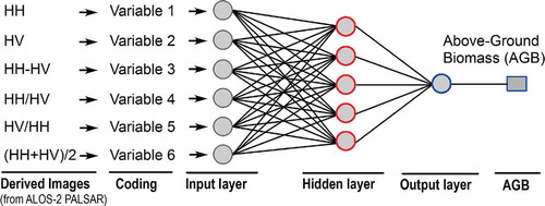
To design the MLPNN model for this study, it was necessary to determine the optimal number of hidden neurons. For this purpose, we used a test suggested by Tien Bui et al. (2016) by varying the numbers of neurons of the MLPNN versus the root-mean-square error (RMSE) using the training data with leave-one-out (LOO) cross-validation techniques. Table 2 shows that the ANN model with five neurons in the hidden layer produced the best performance (the highest R², and the lowest RMSE and mean absolute error, MAE); therefore, the hidden layer with five neurons was selected for use in this study. The final structure of the MLPNN model for this study is shown in Figure 4. The learning rate, momentum, and training iteration were selected as 0.3, 0.2, and 500, respectively (Sasikala, Appavu Alias Balamurugan, and Geetha 2014). The activation function is the logistic sigmoid as suggested by Şenkal and Kuleli (2009).

Table 2. Performance of MLPNN with different number of neurons in the hidden layer.

Number of neurons in hidden layer	R^2	RMSE	MAE
1	0.510	0.403	0.296
2	0.029	0.685	0.526
3	0.177	0.694	0.514
4	0.357	0.591	0.448
5	0.776	0.299	0.237
6	0.480	0.573	0.388
7	0.274	0.766	0.441
8	0.286	0.746	0.44
9	0.325	0.700	0.418
10	0.196	0.839	0.479
11	0.238	0.714	0.431
12	0.194	0.855	0.525
13	0.151	0.872	0.513
14	0.303	0.764	0.403
15	0.174	0.890	0.509

3.2 Performance assessment

We used RMSE, MAE, and coefficient of determination (R²) to assess and compare the performance of the biomass estimation models. These statistical measures are widely used in biomass modeling to evaluate discrepancies between measured data (AGB inventories) and predicted AGB data (Viana et al. 2012; Byrd et al. 2014).

RMSE (Equation (4)) is a standard metric for measuring errors of regression models, but it is strongly influenced by large values and outliers (Chai and Draxler 2014). Therefore, MAE (Equation (5)) is suggested for use with RMSE for determining the variation of model errors (Tien Bui et al. 2016). Lower RMSE and MAE values mean a better model. In addition, a smaller difference between RMSE and MAE means a smaller variance of errors. R² is estimated using Equation (6); higher R² values also mean a better model (Jachowski et al. 2013):

(4)

(5)

(6)

where is the estimated AGB value from the model, is the measured AGB value, n is the total sample used, and are the mean values of the estimated AGB and the measured AGB, respectively.

To select the best model among different machine learning methods, we used Akaike’s Information Criterion (AIC) and Bayesian Information Criterion (BIC) to determine which regression model gives the most accurate estimates (Zucchini 2000; Claeskens and Hjort 2008; Schwarz 2011). Both AIC and BIC provide simple and effective methods for selecting and comparing regression models (Burnham and Anderson 2004; Burnham, Anderson, and Huyvaert 2011). Kelloway (2014) reported that lower AIC values indicated a better-fitting model.

AIC and BIC have been widely used for selecting and comparing different regression models related to the estimation of forest structures and biomass in recent studies (Laurin et al. 2014; Ibanez et al. 2016; Tesfamichael and Beech 2016). We calculated AIC and BIC using Equations (7) and (8). Models were ranked from the lowest to the highest AIC and BIC scores; the model with the lowest AIC and BIC values was considered the best:

(7)

(8)

where SSE is the sum of squares errors, n is the number of sampling plots, and K is the number of parameters; K = p + 1, where p is the number of predictors.

4. Results and discussion

4.1 Field survey results

A total of 1508 mangrove trees were recorded in the 18 sampling plots. We chose only 18 plots because plot collection is time-consuming and there were labor constraints during the field measurement. Two factors in particular that resulted in a small number of sampling plots were the high density of the mangrove forests and their pneumatophores in the study area, and the considerable impact of tidal inundation.

Despite the limited sample plots, we consider our analyses reliable due to the use of machine learning techniques such as MLPNN and LOO cross-validation. These approaches emphasize that small datasets exist in many real-world problems; data-mining methods work well in such circumstances because they do not require statistical distribution assumptions. These issues were discussed in detail in Wisz et al. (2008) and Patel, Khalaf, and Aizenstein (2016). The effects of sample sizes were discussed in Wisz et al. (2008).

Tree counts ranged from 42 to 126 trees per plot, while tree density averaged 79 (Table 3). Total AGB in each 900 m² plot ranged from 620 to 14,634 kg (median = 4447 kg). BGB estimated in each plot ranged from 823 to 29,492 kg (median = 6472 kg). The overall ratio of BGB/AGB was 1.46, calculated using the average BGB (Mg ha⁻¹) and AGB (Mg ha⁻¹) of all 18 recorded sampling plots. This number is comparable to that reported by Komiyama, Ong, and Poungparn (2008).

Table 3. Characteristics of S. caseolaris in the study site.

Plot ID	Tree density (No./900 m^2)	DBH (cm)	Age (years)	Tree height (meter)	AGB (kg/900 m^2)	Root weight (kg/900 m^2)	BGB (kg/900 m^2)	AGB (Mg ha^−1)	BGB (Mg ha^−1)
1	57	10.67	17	5.71	542.91	7.709	823.444	6.887	9.149
2	45	13.22	17	6.42	699.36	9.309	1045.777	8.496	11.620
3	72	11.98	10	6.06	890.00	8.787	1345.252	11.049	14.947
4	83	11.49	10	6.08	956.30	6.992	1414.689	11.686	15.719
5	110	11.81	10	4.85	1085.77	5.093	1992.168	13.347	22.135
6	98	12.06	10	5.33	1094.05	6.663	1859.210	13.517	20.658
7	42	18.79	17	5.67	1099.30	7.655	2131.574	12.844	23.684
8	48	23.07	17	6.56	2077.34	11.480	3843.674	24.015	42.707
9	65	21.18	17	6.67	2442.24	11.006	4302.659	28.328	47.807
10	84	19.02	17	10.30	3846.09	15.965	4378.573	44.181	48.651
11	54	31.58	17	6.33	3976.38	12.977	8679.311	45.412	96.437
12	56	28.84	23	12.40	6409.29	26.660	7356.972	72.552	81.744
13	126	20.42	23	11.00	6955.34	18.150	7689.924	79.592	85.444
14	105	26.11	17	8.64	7264.79	22.896	11066.636	83.812	122.963
15	115	26.25	17	8.17	7632.43	18.383	12261.683	87.680	136.241
16	63	29.25	22	13.40	7928.94	31.490	8538.093	89.744	94.868
17	117	21.82	22	12.50	8162.52	28.125	8271.390	93.620	91.904
18	89	43.75	23	8.00	14535.88	8.800	29492.032	162.598	327.689
Average	79	21.18	17	8.10	4311.052	14.341	6471.837	49.409	71.909

4.2 Characteristics analysis of S. caseolaris in the study area

A correlation matrix summarizing the relationship between various biophysical parameters of S. caseolaris in the study area (Table 4) shows that apart from tree density, all biophysical parameters of S. caseolaris are well correlated. We acquired information on tree age with the help of village security guard teams during the field work.

Table 4. Pearson’s correlation matrix of various biophysical parameters of S. caseolaris (N = 18).

	Tree density	DBH	Height	Age	Tree weight	Root weight	Total AGB
Tree density	1
DBH	0.016	1
Height	0.244	0.459	1
Age	−0.007	0.703**	0.760**	1
Tree weight	0.421	0.644**	0.644**	0.731**	1
Root weight	0.204	0.454	0.929**	0.673**	0.580*	1
Total AGB	0.421	0.846**	0.747**	0.734**	0.933**	0.726**	1

Note: **Correlation is significant at the 0.01 level, *correlation is significant at the 0.05 level.

We observed a strong positive relationship between biophysical parameters of S. caseolaris and AGB, with the exception of tree density. One possible explanation for this might be that tree density is a conditional parameter and depends on the seedling species used. In contrast, low correlations are observed with tree density, reflecting a decrease in the number of trees in the region. During the typhoon season, it is common for S. caseolaris to be felled by storms, normally at the juvenile stage when their pneumatophores have not grown enough and C. stellatus which can be found frequently in the coast of Hai Phong (Marchand 2008).

We analyzed ALOS-2 PALSAR with HH and HV polarizations in order to examine their relationships with different biophysical parameters of S. caseolaris (Table 5).

Table 5. Person’s correlation matrix between backscattering coefficient σ° and various biophysical parameters of S. caseolaris (N = 18).

	HH	HV	Tree density	DBH	Height	Age	Tree weight	Root weight	Total AGB
HH	1
HV	0.878	1
Tree density	0.291	0.341	1
DBH	0.392	0.401	−0.126	1
Height	0.368	0.559*	0.181	0.527*	1
Age	0.481	0.548*	0.028	0.707**	0.798**	1
Tree weight	0.412	0.497	0.276	0.836**	0.693**	0.776**	1
Root weight	0.347	0.432	0.849**	0.101	0.455	0.267	0.469	1
Total AGB	0.334	0.537*	0.431	0.846**	0.747**	0.734**	0.933**	0.726**	1

Note: **Correlation is significant at the 0.01 level, *correlation is significant at the 0.05 level.

L-band backscatterings (σ°) for HH and HV polarizations show a positive relationship with biophysical parameters of S. caseolaris. However, the sensitivity of (σ°) at HV polarization is higher than that of (σ°) at HH polarization. This is likely due to an increase in volume scattering with the growth of S. caseolaris. The wavelength of the ALOS-2 PALSAR system determines the volume scattering and surface scattering. The radar system of the ALOS-2 sensor is dominated by volume scattering from large-scale mangrove forest canopy features and surface scattering from the terrain surface. When the volume of scattering is high, the ALOS-2 PALSAR sensor signal saturates (Le Toan et al. 1992).

This study also determined the relationship between the biophysical parameters of dominant mangrove species in Hai Phong city in 2015 and the backscattering coefficients at HH and HV polarizations (Table 4). A high correlation was observed between the mean backscattering coefficients at HV polarization and various biophysical parameters such as: tree height, age, and apart from tree density for S. caseolaris. The HV shows a higher correlation than HH for S. caseolaris where the volumetric scattering might strengthen the cross-polarization (Mougin et al. 1999; Proisy et al. 2000).

4.3 Modeling results, assessment, and comparison

Since the sample size was small, the LOO cross-validation technique was used for building prediction models. This is an effective technique that has ability to eliminate bias in estimations of model performance (Moore 2001). This technique allows each sample to be excluded while a model is developed with all remaining samples and used to predict the excluded sample. Accordingly, a total of 18 sub-models were developed using the MLPNN techniques; the final MLPNN model was generated by averaging the 18 sub-models.

The performance of the final MLPNN model is shown in Table 6. The RMSE value (0.299) is significantly lower than the standard deviation of the AGB inventories (0.425) indicating that the model performed well with the data. The MAE (0.237) is slightly lower than the RMSE indicating that the error variation is small. The R² value (0.776) indicates a satisfactory result. Overall, the MLPNN model performed well in this study area.

Table 6. Machine learning models with leave-one-out (LOO) cross-validation for estimation of above-ground biomass in this study.

No.	Machine learning model	RMSE	MAE	R^2
1	Multi-layer perceptron neural networks (MLPNN)	0.299	0.237	0.776
2	Support vector regression (SVR)	0.359	0.268	0.596
3	Radial basis function neural networks (RBFNN)	0.388	0.333	0.612
4	Gaussian process (GP)	0.379	0.345	0.483
5	Random forests (RF)	0.402	0.364	0.372

As the purpose of this study was to estimate the AGB of S. caseolaris in coastal Vietnam, the usability of the MLPNN model should be assessed and confirmed in its effectiveness. We selected the support vector regression (SVR), radial basis function neural network (RBFNN), Gaussian process (GP), and random forests (RF) models for comparison. SVR was selected because it outperforms various machine learning models in estimating AGB (Jachowski et al. 2013) whereas the others are widely used soft computing models with high performance in many fields (Mountrakis, im, and Ogole 2011; Were et al. 2015; Valipour 2016).

SVR is a regression version of the popular support vector machines that was developed based on statistical learning theory (Smola and Vapnik 1997). In this study, we used SVR with the radial basis function kernel (Hoang, Bui, and Liao 2016) and the SMO algorithm (Were et al. 2015). Accordingly, the best values for the kernel width (0.195) and the regularization (2.75) were found using the grid search method. For RBFNN (Chen and Chen 1995), the best structure (6 input neurons, one hidden layer with 10 clusters, and one output) was found based on a test suggested in Hong et al. (2015). For GP, the radial basis function (Scholkopf et al. 1997) was used with gamma of 4.185 as the best value for the study area. The RF (Breiman 2001) model with 60 trees had the highest performance for this study area.

The modeling results for estimating the AGB of S. caseolaris using the four machine-learning models (SVR, RBFNN, GP, and RF) with the LOO cross-validation technique are shown in Table 6. Among the four machine-learning models, the SVR model had the highest performance: RMSE, MAE, and R² were 0.359, 0.268, and 0.596, respectively. However, the performance of the SVR model was clearly lower than the MLPNN model in this study (Table 6). In contrast to the SVR model, the RF model had the lowest performance: RMSE, MAE, and R² were 0.402, 0.364, and 0.372, respectively. In addition, the MLPNN model had the lowest AIC and BIC values among the five machine learning models (Table 7). Therefore we conclude that the MLPNN model achieved the best performance in this study for estimating the AGB of S. caseolaris.

Table 7. Comparison of MLPNN, SVR, RBFNN, GP, and RF models, using AIC and BIC.

	MLPNN	SVR	RBFNN	GP	RF
AIC	−29.473	−22.745	−20.101	−20.510	−18.151
BIC	−23.240	−16.512	−13.868	−14.278	−11.918

4.4 Generation of the AGB map and its analysis

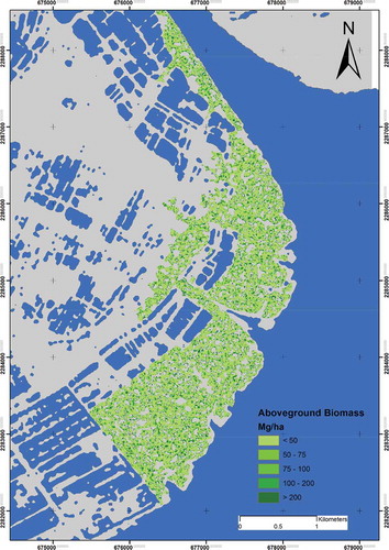
Since the MLPNN model was the best suited for the data, we used it to estimate the AGB of S. caseolaris for the study area; the results were then converted to a GIS format for use in ArcGIS 10.2. The resulting map visualized five classes (Figure 5) showing that the AGB ranged between 2.78 and 298.95 ± 1.99 Mg ha⁻¹, with an average of 55.80 ± 1.99 Mg ha⁻¹; the highest biomass was located in the Northeast region. These results showed that the estimation of AGB spatial distribution generated by the MLPNN model was consistent with the measured mean, though the AGB range was higher than the actual distribution range (Table 3). This was likely due to the saturation level of the L-band ALOS-2 PALSAR sensor in estimating the biomass of mangrove forests. The estimated biomass of S. caseolaris was mainly distributed in the high tidal zones. The experimental results matched our field observations, as this species can grow well in high tidal inundation level due to its pneumatophores (Figure 4(c) and (d)).

Figure 5. Spatial distribution pattern of biomass in the study area.

Our estimate of the mangroves’ BGB (using the previously defined 1.46 BGB/AGB ratio) yielded a range between 4.06 and 436.47 ± 2.91 Mg ha⁻¹, with an average of 81.47 ± 2.91 Mg ha⁻¹. The total biomass of S. caseolaris in the study area, derived by a combination of AGB and BGB, ranged from 6.85 to 735.42 Mg ha⁻¹, with an average of 137.27 Mg ha⁻¹. Using the 0.47 conversion factor between total biomass and carbon stock (Howard et al. 2014), we estimated that the total carbon stock of S. caseolaris in the study area ranged from 3.22 to 345.65 Mg C ha⁻¹, with an average of 64.52 Mg C ha⁻¹. This number is different from the results reported by Hamdan et al. (2013) and Vu, Takeuchi, and Van (2014) probably because these studies calculated the carbon stock of Matang mangroves in Malaysia and Quang Ninh province, Vietnam, based solely on AGB. We, therefore, suggest further study with more focus on carbon stock estimation derived from both AGB and BGB. In addition, our estimate is much lower than that for mangrove ecosystems in the Mekong Delta region since they belong to a biosphere reserve and protected area (Nam et al. 2016).

Previous studies have found that polarimetric radar signatures at long wavelengths such as the L- and P-bands were most sensitive to different mangrove species along the coast of French Guiana. This research pointed out that the backscattering coefficients of HV polarization at L- and P-bands reached the highest correlations with most mangrove parameters (Proisy et al. 2000). However, the correlation coefficients of different regression models were limited. Recent studies using ALOS PALSAR to estimate the AGB of Matang mangroves in Malaysia found that HV backscatter gave the best correlation coefficient between polarimetric ALOS PALSAR backscattering and AGB for the three dominant species R. apiculata, A. alba, and B. parviflora, though the accuracy of the model (R² = 0.427) was relatively low (Hamdan, Khali Aziz, and Mohd Hasmadi 2014). Multi-linear regression is the most commonly used method for estimating the AGB of mangrove forests in previous studies (Proisy, Couteron, and Fromard 2007; Hamdan, Khali Aziz, and Mohd Hasmadi 2014; Hirata et al. 2014). However, the performance of this model was relatively low with an R² value less than 0.6. Thus, the development of more accurate models for estimating mangrove biomass is necessary to promote the implementation of MRV strategies and developing national REDD+ mechanisms. Our results suggest that a combination of multi-polarizations generated in MNPNN can perform better than traditional models (R² = 0.776).

Prior studies reported that the saturation level of AGB in mangrove forests was at over 100 Mg ha⁻¹ (Lucas et al. 2007) and 150 Mg ha⁻¹ (Hamdan, Khali Aziz, and Mohd Hasmadi 2014) because of differences in the root systems and tidal inundation level of different tropical mangrove species. Therefore, MLPNNs likely over-estimate biomass at low observed values and under-estimate at high observed values. This may explain why errors occur largely at very high biomass values. The biomass of plots containing dense large mangrove trees with high DBH is likely under-estimated using machine learning algorithms. Despite these limitations of SAR data, our findings show that the ALOS-2 PALSAR L-band, with high sensitive mode and backscattering coefficients at HH and HV polarizations, was sensitive to AGB, exceeding 100 Mg ha⁻¹ for S. caseolaris. This means that the backscattering coefficients at HH and HV polarizations remain stable when the AGB of S. caseolaris reaches over 100 Mg ha⁻¹. The saturation level of mangrove species of Hai Phong is slightly lower than that of mangrove forests in Malaysia due to differences in stand age, growth stage, and species (Hamdan, Khali Aziz, and Mohd Hasmadi 2014). Backscattering in HH and HV polarizations of ALOS-2 PALSAR increased when biomass was below 100 Mg ha⁻¹. Backscattering in HH and HV polarizations increased when biomass was below 100 Mg ha⁻¹. The backscattering was then saturated after the biomass of mangrove species increased further. This is likely due to an increased extinction of radar signals caused by the mangrove canopy (Le Toan et al. 2004).

Data saturation, which occurs in both optical and SAR sensor data, is an important factor influencing the accuracy of biomass estimation. Previous studies have reported that data saturation is one of the major problems resulting in low performance by optical data sensors when estimating AGB for areas with high biomass or high canopy density. The saturation level of optical sensors such as Landsat TM reaches about 100–150 tons ha⁻¹ in complex moist tropical forests (Foody, Boyd, and Cutler 2003).

Saturation is also a common problem for SAR sensors when estimating biomass in a study area with complex forest stand structure (Mitchard et al. 2009; Lucas et al. 2009). A short wavelength such as C-band at 6 cm saturates often at 10 kg/m² while long wavelengths such as L- and P-bands saturate often at 100 tons ha⁻¹ for a complex and mixed forest structure; this saturation number rises to roughly 250 tons ha⁻¹ for simple forests with a few dominant species (Ranson and Sun 1994). Shugart, Saatchi, and Hall (2010) pointed out that the L-band saturation point is at around 100–150 tons ha⁻¹ while P-band could be sensitive for biomass estimation at a saturation level of 100–300 tons ha⁻¹, depending on the forest types (FAO 2009). The saturation level of the ALOS-2 PALSAR sensor for AGB estimation of S. caseolaris in this study was around 100 Mg ha⁻¹, which is consistent with the results reported by Lucas et al. (2007) and Hamdan, Khali Aziz, and Mohd Hasmadi (2014). More research is, therefore, needed to reduce the data saturation problem through the use of multi-source data or data fusion (Basuki et al. 2013; Luo et al. 2017).

4.5 Biomass estimation using remotely sensed data and machine learning methods

Light detection and ranging (LiDAR) is an active remote-sensing sensor that utilized a pulsed laser to measure ranges and examine the surface of the Earth (Lefsky et al. 2002). LiDAR data have an important role in estimating AGB since LiDAR pulses can penetrate certain vegetation canopy (Gleason and Im 2011), especially in tropical areas where frequent cloud conditions occur. Several studies have used LiDAR data for estimating the canopy height of mixed forest (Nilsson 1996; Zimble et al. 2003) and mangrove forests, in combination with Shuttle Radar Topography Mission data (SRTM) (Simard et al. 2006) or together with LANDSAT ETM+ imagery (Fatoyinbo et al. 2008).

Direct biomass estimation methods using airborne LiDAR can offer higher accuracy in tree extraction (Lee, Kim, and Choi 2013), estimating number of trees and tree height (Unger et al. 2014), and AGB than methods using radar and optical data (Zolkos, Goetz, and Dubayah 2013) because LiDAR can characterize both horizontal and vertical canopy structure (Lu et al. 2016). Recent studies have indicated the potential of using LiDAR data with SAR data to map height and biomass of mangrove forest (Simard et al. 2006), and hyperspectral imagery for both AGB and BGB (Luo et al. 2017). However, LiDAR data are still captured in small and geographically limited areas and may be more costly than data obtained from space-borne resources for a large area. Analyzing data derived from LiDAR requires more skills, knowledge, and specific software (Lu 2006). In addition, LiDAR has limited spectral information due to the one wavelength of laser point intensity (Lu et al. 2016).

Compared with LiDAR metrics, space-borne hyperspectral sensors offer a broader data set by providing a large number of spectral bands from visible to near infrared (NIR) or shortwave infrared (SWIR). These have great potential for classifying vegetation cover and estimating vegetation biomass comparing to other multispectral sensors. For example, Sibanda, Mutanga, and Rouget (2016) reported that hyperspectral data can provide slightly higher accuracies in estimating grass biomass than Sentinel 2 multispectral imager (MSI) data. However, Vaglio Laurin et al. (2014) claimed that hyperspectral data alone had limited prediction ability in estimating forest biomass (R² = 0.36). In addition, hyperspectral data are mainly space-borne and captured in small and geographically limited (Lu 2006).

With the launch of new space-borne satellite sensors such as RapidEye, Sentinel, TerraSAR-X, and ALOS-2 PALSAR (with high spatial, temporal, and spectral resolution), the issue of limited areas associated with airborne remote sensing can be overcome by encouraging new approaches to developing more accurate models for AGB estimation. The development of data mining and machine learning methods for biomass estimation has real potential in this regard, resulting in an increased use of machine learning methods for forest biomass estimation.

Several machine learning methods have been used for AGB estimation in the past few years, including k-NN, ANN, SVR, and RF (Jachowski et al. 2013; Dube et al. 2014; Ali et al. 2015; Wu et al. 2016). Machine learning models have shown their ability to estimate forest biomass by using optical and SAR sensors and by data fusion of multi-source data. These approaches have been also compared to other parametric approaches, showing that in most cases, machine learning methods have outperformed conventional methods (Ali et al. 2015). Recently, several studies showed the potential of the stochastic gradient boosting (SGB) algorithm for AGB estimation by using both optical sensors from medium resolution (Güneralp, Filippi, and Randall 2014) to high resolution (Dube et al. 2014), and SAR data (Carreiras, Melo, and Vasconcelos 2013).

Other recent approaches using machine learning and remote sensing consider data from multi-sensors in order to improve performance. For example, Shataee Joibary (2013) studied the application of non-parametric models (k-NN, SVR, RF, and ANN) for the estimation of forest volume and basal area based on airborne LiDAR and Landsat TM data. The results show that SVR performed better than the other models when LiDAR and Landsat TM data were combined. More recently, another study in southwest Thailand (Jachowski et al. 2013) used GeoEye-1 and ASTER with the SVM model for mangrove biomass estimation, showing a promising result (R² = 0.66). Integration of LiDAR and hyperspectral or multi-source data can therefore improve biomass estimation significantly with relatively high accuracy (Anderson et al. 2008; Vaglio Laurin et al. 2014; Luo et al. 2017). Thus, the use of machine learning techniques in combination with multi-source data or data fusion should be investigated further in order to acquire more precise biomass maps.

5. Concluding remarks

This study investigated the applicability of using ALOS-2 PALSAR data with the MLPNN model for estimating the AGB of S. caseolaris in the coastal area of Hai Phong city, Vietnam, and compared performance of the MLPNN with other machine learning algorithms. Our findings show that the MLPNN model produced more accurate biomass estimates than other machine learning models. AGB and BGB for this species were estimated from 2.78 to 298.95 Mg ha⁻¹ (with an average of 55.8 Mg ha⁻¹) and 4.06 to 436.47 Mg ha⁻¹(with an average of 81.47 Mg ha⁻¹), respectively, using LOO cross-validation with an RMSE of 0.299, an MAE of 0.237, and R² of 0.776. The total carbon stock in the study area was estimated between 3.22 and 345.65 Mg C ha⁻¹ (with an average of 64.52 Mg C ha⁻¹). Our study also illustrated the use of ALOS-2 PALSAR data in high sensitive mode together with machine learning algorithms for characterizing the spatial distribution of mangrove biomass and determined the relationship between the biophysical parameters of a dominant mangrove species and backscattering coefficients at HH and HV polarizations. We conclude that ALOS-2 PALSAR can be used with MLPNN in estimating mangrove biomass and carbon stock. Despite the limitations caused by saturation levels of AGB for S. caseolaris over 100 Mg ha⁻¹, the use of L-band ALOS-2 PALSAR in high sensitive mode with machine learning provides an alternative approach that may allow rapid estimation of biomass for different mangrove species and their carbon stock in the tropics where accessibility is limited in large areas.

Our results show that MNPNN models provide an alternative method to derive mangrove biomass in a cost-effective and practical way. The machine learning algorithms and methods used in this research can be replicated for other mangrove forest species with similar characteristics, stand structures, and other biophysical parameters. Our approach, using ALOS-2 PALSAR in high sensitive mode together with machine learning algorithms, can be used as a practical guide for the preliminary design of regional and local biomass assessment in other regions of Vietnam. Further research is needed to determine the biomass of other mangrove species and extend this work for entire mangrove forests in Vietnam. The findings will provide useful information regarding the spatial distribution of biomass for S. caseolaris and its carbon stock. This will support provincial decision-making on mangrove conservation and management.

Highlights

• Multi-layer perceptron neural networks (MLPNN) model performs well (R² = 0.776).

• MLPNN model outperforms the machine learning techniques in above-ground biomass estimation of Sonneratia caseolaris.

• ALOS-2 PALSAR (HH and HV polarization) can be used with MLPNN in estimating mangrove forest biomass.

Acknowledgments

The authors would like to thank CARES (Center for Agricultural Researches and Ecological Studies), Vietnam National University of Agriculture (VNUA), Vietnam for logistical support during fieldwork. We are highly thankful to MEXT (Ministry of Education, Culture, Sports, Science, and Technology), Japanese Government for financial support to pursue a PhD degree at the University of Tsukuba, Japan.

Disclosure statement

No potential conflict of interest was reported by the authors.

Additional information

Funding

This work was supported by MEXT (Ministry of Education, Culture, Sports, Science, and Technology).

References

- Ali, I., F. Greifeneder, J. Stamenkovic, M. Neumann, and C. Notarnicola. 2015. “Review of Machine Learning Approaches for Biomass and Soil Moisture Retrievals from Remote Sensing Data.” Remote Sensing 7 (12): 16398–16421. doi:10.3390/rs71215841.
- Alongi, D. M. 2002. “Present State and Future of the World’s Mangrove Forests.” Environmental Conservation 29 (03): 331–349. doi:10.1017/S0376892902000231.
- Anderson, J. E., L. C. Plourde, M. E. Martin, B. H. Braswell, M.-L. Smith, R. O. Dubayah, M. A. Hofton, and J. B. Blair. 2008. “Integrating Waveform Lidar with Hyperspectral Imagery for Inventory of a Northern Temperate Forest.” Remote Sensing of Environment 112 (4): 1856–1870. doi:10.1016/j.rse.2007.09.009.
- Basuki, T. M., A. K. Skidmore, Y. A. Hussin, and I. Van Duren. 2013. “Estimating Tropical Forest Biomass More Accurately by Integrating ALOS PALSAR and Landsat-7 ETM+ Data.” International Journal of Remote Sensing 34 (13): 4871–4888. doi:10.1080/01431161.2013.777486.
- Beh Boon, C., M. Z. M. Jafri, and S. L. Hwee. 2011. “Mangrove Mapping in Penang Island by Using Artificial Neural Network Technique.” Paper presented at the Open Systems (ICOS), 2011 IEEE Conference on, September 25–28.
- Breiman, L. 2001. “Random Forests.” Machine Learning 45 (1): 5–32. doi:10.1023/a:1010933404324.
- Bui, D., B. P. Pradhan, H. Nampak, Q.-T. Bui, Q.-A. Tran, and Q.-P. Nguyen. 2016. “Hybrid Artificial Intelligence Approach Based on Neural Fuzzy Inference Model and Metaheuristic Optimization for Flood Susceptibility Modeling in a High-Frequency Tropical Cyclone Area Using GIS.” Journal of Hydrology 540: 317–330. doi:10.1016/j.jhydrol.2016.06.027.
- Burnham, K. P., and D. R. Anderson. 2004. “Multimodel Inference Understanding AIC and BIC in Model Selection.” Sociological Methods & Research 33 (2): 261–304. doi:10.1177/0049124104268644.
- Burnham, K. P., D. R. Anderson, and K. P. Huyvaert. 2011. “AIC Model Selection and Multimodel Inference in Behavioral Ecology: Some Background, Observations, and Comparisons.” Behavioral Ecology and Sociobiology 65 (1): 23–35. doi:10.1007/s00265-010-1029-6.
- Byrd, K. B., J. L. O’Connell, S. Di Tommaso, and M. Kelly. 2014. “Evaluation of Sensor Types and Environmental Controls on Mapping Biomass of Coastal Marsh Emergent Vegetation.” Remote Sensing of Environment 149: 166–180. doi:10.1016/j.rse.2014.04.003.
- Carreiras, J., J. Melo, and M. Vasconcelos. 2013. “Estimating the Above-Ground Biomass in Miombo Savanna Woodlands (Mozambique, East Africa) Using L-Band Synthetic Aperture Radar Data.” Remote Sensing 5 (4): 1524–1548. doi:10.3390/rs5041524.
- Chai, T., and R. R. Draxler. 2014. “Root Mean Square Error (RMSE) or Mean Absolute Error (Mae)?–Arguments against Avoiding RMSE in the Literature.” Geoscientific Model Development 7 (3): 1247–1250. doi:10.5194/gmd-7-1247-2014.
- Chave, J., C. Andalo, S. Brown, M. A. Cairns, J. Q. Chambers, D. Eamus, H. Fölster, et al. 2005. “Tree Allometry and Improved Estimation of Carbon Stocks and Balance in Tropical Forests.” Oecologia 145 (1): 87–99. doi:10.1007/s00442-005-0100-x.
- Chen, T., and H. Chen. 1995. “Approximation Capability to Functions of Several Variables, Nonlinear Functionals, and Operators by Radial Basis Function Neural Networks.” Ieee Transactions on Neural Networks 6 (4): 904–910. doi:10.1109/72.392252.
- Civco, D. L. 1993. “Artificial Neural Networks for Land-Cover Classification and Mapping.” International Journal of Geographical Information Systems 7 (2): 173–186. doi:10.1080/02693799308901949.
- Claeskens, G., and N. L. Hjort. 2008. Model Selection and Model Averaging. Vol. 330. Cambridge: Cambridge University Press.
- Clough, B. F., P. Dixon, and O. Dalhaus. 1997. “Allometric Relationships for Estimating Biomass in Multi-Stemmed Mangrove Trees.” Australian Journal of Botany 45 (6): 1023–1031. doi:10.1071/BT96075.
- Clough, B. F., and K. Scott. 1989. “Allometric Relationships for Estimating Above-Ground Biomass in Six Mangrove Species.” Forest Ecology and Management 27 (2): 117–127. doi:10.1016/0378-1127(89)90034-0.
- Conchedda, G., L. Durieux, and P. Mayaux. 2008. “An Object-Based Method for Mapping and Change Analysis in Mangrove Ecosystems.” ISPRS Journal of Photogrammetry and Remote Sensing 63 (5): 578–589. doi:10.1016/j.isprsjprs.2008.04.002.
- Danielsen, F., M. K. Sørensen, M. F. Olwig, V. Selvam, F. Parish, N. D. Burgess, T. Hiraishi, et al. 2005. “The Asian Tsunami: A Protective Role for Coastal Vegetation.” Science 310: 643. doi:10.1126/science.1118387.
- Darmawan, S., W. Takeuchi, Y. Vetrita, K. Wikantika, and D. K. Sari. 2015. “Impact of Topography and Tidal Height on ALOS PALSAR Polarimetric Measurements to Estimate Aboveground Biomass of Mangrove Forest in Indonesia.” Journal of Sensors 2015: 1–13. doi:10.1155/2015/641798.
- Dat, P. T., and K. Yoshino. 2011. “Monitoring Mangrove Forest Using Multi-Temporal Satellite Data in the Northern Coast of Vietnam.” Paper presented at The 32nd Asian Conference on Remote Sensing, Taipei, Taiwan, October 3–7.
- De Leeuw, M. R., and L. M. T. De Carvalho. 2009. “Performance Evaluation of Several Adaptive Speckle Filters for SAR Imaging.” Anais XIV Simpósio Brasileiro De Sensoriamento Remoto, Natal, April 25-30, 7299–7305. http://marte.sid.inpe.br/col/dpi.inpe.br/sbsr@80/2008/11.18.12.44/doc/7299-7305.pdf
- Donato, D. C., J. Boone Kauffman, D. Murdiyarso, S. Kurnianto, M. Stidham, and M. Kanninen. 2011. “Mangroves among the Most Carbon-Rich Forests in the Tropics.” Nature Geosci 4 (5): 293–297. doi:10.1038/ngeo1123.
- Dube, T., O. Mutanga, A. Elhadi, and R. Ismail. 2014. “Intra-And-Inter Species Biomass Prediction in a Plantation Forest: Testing the Utility of High Spatial Resolution Spaceborne Multispectral Rapideye Sensor and Advanced Machine Learning Algorithms.” Sensors 14 (8): 15348–15370. doi:10.3390/s140815348.
- Duke, N. C., J.-O. Meynecke, S. Dittmann, A. M. Ellison, K. Anger, U. Berger, S. Cannicci, et al. 2007. “A World Without Mangroves?.” Science 317 (5834): 41–42. doi:10.1126/science.317.5834.41b.
- Ellison, A. M. 2002. “Macroecology of Mangroves: Large-Scale Patterns and Processes in Tropical Coastal Forests.” Trees 16 (2–3): 181–194. doi:10.1007/s00468-001-0133-7.
- FAO. 2007. “The World’s Mangroves 1980-2005. A Thematic Study Prepared in the Framework of the Global Forest Resources Assessment 2005.” FAO Forestry Paper, 89. Rome: Food and Agriculture Organization of the United Nations.
- FAO. 2009. “GTOS: Biomass Assessment of the Status of the Development of the Standards for the Terrestrial Essential Climate Variables.” 18p. Rome, Italy.
- Fatoyinbo, T. E., M. Simard, R. A. Washington-Allen, and H. H. Shugart. 2008. “Landscape-Scale Extent, Height, Biomass, and Carbon Estimation of Mozambique’s Mangrove Forests with Landsat ETM+ and Shuttle Radar Topography Mission Elevation Data.” Journal of Geophysical Research: Biogeosciences 113 (G2). doi:10.1029/2007JG000551.
- Foody, G. M., D. S. Boyd, and M. E. J. Cutler. 2003. “Predictive Relations of Tropical Forest Biomass from Landsat TM Data and Their Transferability between Regions.” Remote Sensing of Environment 85 (4): 463–474. doi:10.1016/S0034-4257(03)00039-7.
- Gleason, C. J., and J. Im. 2011. “A Review of Remote Sensing of Forest Biomass and Biofuel: Options for Small-Area Applications.” Giscience & Remote Sensing 48 (2): 141–170. doi:10.2747/1548-1603.48.2.141.
- Güneralp, İ., A. M. Filippi, and J. Randall. 2014. “Estimation of Floodplain Aboveground Biomass Using Multispectral Remote Sensing and Nonparametric Modeling.” International Journal of Applied Earth Observation and Geoinformation 33: 119–126. doi:10.1016/j.jag.2014.05.004.
- Hall, M., E. Frank, G. Holmes, B. Pfahringer, P. Reutemann, and I. H. Witten. 2009. “The WEKA Data Mining Software: An Update.” SIGKDD Explor. Newsl. 11 (1): 10–18. doi:10.1145/1656274.1656278.
- Hamdan, O., M. R. Khairunnisa, A. A. Ammar, I. Mohd Hasmadi, and H. Khali Aziz. 2013. “Mangrove Carbon Stock Assessment by Optical Satellite Imagery.” Journal of Tropical Forest Science 25 (4): 554–565.
- Hamdan, O., H. Khali Aziz, and I. Mohd Hasmadi. 2014. “L-Band ALOS PALSAR for Biomass Estimation of Matang Mangroves, Malaysia.” Remote Sensing of Environment 155: 69–78. doi:10.1016/j.rse.2014.04.029.
- Haykin, S. 1998. Neural Networks: A Comprehensive Foundation. 2nd ed. Upper Saddle River, NJ, USA: Prentice Hall.
- Heumann, B. W. 2011. “Satellite Remote Sensing of Mangrove Forests: Recent Advances and Future Opportunities.” Progress in Physical Geography 35 (1): 87–108. doi:10.1177/0309133310385371.
- Hirata, Y., R. Tabuchi, P. Patanaponpaiboon, S. Poungparn, R. Yoneda, and Y. Fujioka. 2014. “Estimation of Aboveground Biomass in Mangrove Forests Using High-Resolution Satellite Data.” Journal of Forest Research 19 (1): 34–41. doi:10.1007/s10310-013-0402-5.
- Hoang, N.-D., D. T. Bui, and K.-W. Liao. 2016. “Groutability Estimation of Grouting Processes with Cement Grouts Using Differential Flower Pollination Optimized Support Vector Machine.” Applied Soft Computing 45: 173–186. doi:10.1016/j.asoc.2016.04.031.
- Hong, H., X. Chong, I. Revhaug, and D. T. Bui. 2015. “Spatial Prediction of Landslide Hazard at the Yihuang Area (China): A Comparative Study on the Predictive Ability of Backpropagation Multi-Layer Perceptron Neural Networks and Radial Basic Function Neural Networks.” In Cartography - Maps Connecting the World, edited by C. R. Sluter, C. B. Madureira Cruz, and P. M. L. de Menezes, 175–188. Cham, Switzerland: Springer International Publishing.
- Hong, P. N., and H. T. San. 1993. “Mangroves of Vietnam.” In Iucn, 173. Bangkok: The International Union for Conservation of Nature and Natural Resources (IUCN).
- Hong, P. N., H. T. San, and P. T. A. Dao. 1998. “The Role of Mangrove Ecosystem in the Environment and the Life of People in Coastal Mangrove Areas.” Paper presented at the Proceedings of the national workshop on Socio-economic status of women in coastal mangrove areas - Trends to improve their lives and environment, Hanoi, 31 Oct–4 Nov 1997.
- Howard, J., S. Hoyt, K. Isensee, E. Pidgeon, and M. Telszewski. 2014. “Coastal Blue Carbon: Methods for Assessing Carbon Stocks and Emissions Factors in Mangroves, Tidal Salt Marshes, and Seagrass Meadows.” In International Union for Conservation of Nature, edited by J. Howard, S. Hoyt, K. Isensee, E. Pidgeon, and M. Telszewski. Arlington, VA: Conservation International, Intergovernmental Oceanographic Commission of UNESCO.
- Ibanez, C. A. G., B. G. Carcellar III, E. C. Paringit, R. J. L. Argamosa, R. A. G. Faelga, M. A. V. Posilero, G. P. Zaragosa, and N. A. Dimayacyac. 2016. “Estimating Dbh of Trees Employing Multiple Linear Regression of the Best Lidar-Derived Parameter Combination Automated in Python in a Natural Broadleaf Forest in the Philippines.” ISPRS-International Archives of the Photogrammetry, Remote Sensing and Spatial Information Sciences XLI-B8: 657–662. doi:10.5194/isprsarchives-XLI-B8-657-2016.
- Jachowski, N. R., M. S. Y. Quak, D. A. Friess, D. A. Duangnamon, E. L. Webb, and A. D. Ziegler. 2013. “Mangrove Biomass Estimation in Southwest Thailand Using Machine Learning.” Applied Geography 45: 311–321. doi:10.1016/j.apgeog.2013.09.024.
- JAXA. 2014. ALOS-2/PALSAR-2 Level 1.1/1.5/2.1/3.1 CEOS SAR Product, 233. Sengen: Japan Aerospace Exploration Agency.
- Jin-Eong, O., G. W. Khoon, and B. F. Clough. 1995. “Structure and Productivity of a 20-Year-Old Stand of Rhizophora Apiculata Bl. Mangrove Forest.” Journal of Biogeography 22 (2/3): 417–424. doi:10.2307/2845938.
- Kauffman, J. B., C. Heider, J. Norfolk, and F. Payton. 2014. “Carbon Stocks of Intact Mangroves and Carbon Emissions Arising from Their Conversion in the Dominican Republic.” Ecological Applications 24 (3): 518–527. doi:10.1890/13-0640.1.
- Kelloway, E. K. 2014. Using Mplus for Structural Equation Modeling: A Researcher’s Guide. Thousand Oaks, CA: SAGE Publications.
- Komiyama, A., V. Jintana, T. Sangtiean, and S. Kato. 2002. “A Common Allometric Equation for Predicting Stem Weight of Mangroves Growing in Secondary Forests.” Ecological Research 17 (3): 415–418. doi:10.1046/j.1440-1703.2002.00500.x.
- Komiyama, A., J. E. Ong, and S. Poungparn. 2008. “Allometry, Biomass, and Productivity of Mangrove Forests: A Review.” Aquatic Botany 89 (2): 128–137. doi:10.1016/j.aquabot.2007.12.006.
- Komiyama, A., S. Poungparn, and S. Kato. 2005. “Common Allometric Equations for Estimating the Tree Weight of Mangroves.” Journal of Tropical Ecology 21 (04): 471–477. doi:10.1017/S0266467405002476.
- Laurin, G., Q. C. Chen, J. A. Lindsell, D. A. Coomes, F. D. Del Frate, L. Guerriero, F. Pirotti, and R. Valentini. 2014. “Above Ground Biomass Estimation in an African Tropical Forest with Lidar and Hyperspectral Data.” ISPRS Journal of Photogrammetry and Remote Sensing 89: 49–58. doi:10.1016/j.isprsjprs.2014.01.001.
- Le Toan, T., A. Beaudoin, J. Riom, and D. Guyon. 1992. “Relating Forest Biomass to SAR Data.” IEEE Transactions on Geoscience and Remote Sensing 30 (2): 403–411. doi:10.1109/36.134089.
- Le Toan, T., S. Quegan, I. Woodward, M. Lomas, N. Delbart, and G. Picard. 2004. “Relating Radar Remote Sensing of Biomass to Modelling of Forest Carbon Budgets.” Climatic Change 67 (2–3): 379–402. doi:10.1007/s10584-004-3155-5.
- Lee, S. J., J. R. Kim, and Y. S. Choi. 2013. “The Extraction of Forest CO2 Storage Capacity Using High-Resolution Airborne Lidar Data.” Giscience & Remote Sensing 50 (2): 154–171. doi:10.1080/15481603.2013.786957.
- Lefsky, M. A., W. B. Cohen, G. G. Parker, and D. J. Harding. 2002. “Lidar Remote Sensing for Ecosystem Studies: Lidar, an Emerging Remote Sensing Technology that Directly Measures the Three-Dimensional Distribution of Plant Canopies, Can Accurately Estimate Vegetation Structural Attributes and Should Be of Particular Interest to Forest, Landscape, and Global Ecologists.” Bioscience 52 (1): 19–30. doi:10.1641/0006-3568(2002)052[0019:lrsfes]2.0.co;2.
- Long, B. G., and T. D. Skewes. 1996. “A Technique for Mapping Mangroves with Landsat TM Satellite Data and Geographic Information System.” Estuarine, Coastal and Shelf Science 43 (3): 373–381. doi:10.1006/ecss.1996.0076.
- Long, J. B., and C. Giri. 2011. “Mapping the Philippines’ Mangrove Forests Using Landsat Imagery.” Sensors 11 (12): 2972–2981. doi:10.3390/s110302972.
- Lu, D. 2006. “The Potential and Challenge of Remote Sensing‐Based Biomass Estimation.” International Journal of Remote Sensing 27 (7): 1297–1328. doi:10.1080/01431160500486732.
- Lu, D., Q. Chen, G. Wang, L. Liu, G. Li, and E. Moran. 2016. “A Survey of Remote Sensing-Based Aboveground Biomass Estimation Methods in Forest Ecosystems.” International Journal of Digital Earth 9 (1): 63–105. doi:10.1080/17538947.2014.990526.
- Lucas, R. M., P. Bunting, D. Clewley, C. Proisy, P. W. M. Souza Filho, K. Viergever, I. Woodhouse, C. Ticehurst, J. Carreiras, and A. Rosenqvist. 2009. Characterisation and Monitoring of Mangroves Using ALOS PALSAR Data. Sengen: JAXA.
- Lucas, R. M., A. L. Mitchell, A. Rosenqvist, C. Proisy, A. Melius, and C. Ticehurst. 2007. “The Potential of L-Band SAR for Quantifying Mangrove Characteristics and Change: Case Studies from the Tropics.” Aquatic Conservation: Marine and Freshwater Ecosystems 17 (3): 245–264. doi:10.1002/aqc.833.
- Luo, S., C. Wang, X. Xiaohuan, F. Pan, D. Peng, J. Zou, S. Nie, and H. Qin. 2017. “Fusion of Airborne Lidar Data and Hyperspectral Imagery for Aboveground and Belowground Forest Biomass Estimation.” Ecological Indicators 73: 378–387. doi:10.1016/j.ecolind.2016.10.001.
- Mahdizadeh Khasraghi, M., M. A. Sefidkouhi, and M. Valipour. 2015. “Simulation of Open- and Closed-End Border Irrigation Systems Using SIRMOD.” Archives of Agronomy and Soil Science 61 (7): 929–941. doi:10.1080/03650340.2014.981163.
- Marchand, M. 2008. Mangrove Restoration in Vietnam: Key Considerations and a Practical Guide. Delft: Deltares.
- Mas, J. F. 2004. “Mapping Land Use/Cover in a Tropical Coastal Area Using Satellite Sensor Data, GIS and Artificial Neural Networks.” Estuarine, Coastal and Shelf Science 59 (2): 219–230. doi:10.1016/j.ecss.2003.08.011.
- Mazda, Y., M. Magi, Y. Ikeda, T. Kurokawa, and T. Asano. 2006. “Wave Reduction in a Mangrove Forest Dominated by Sonneratia Sp.” Wetlands Ecology and Management 14 (4): 365–378. doi:10.1007/s11273-005-5388-0.
- Mazda, Y., M. Magi, M. Kogo, and P. N. Hong. 1997. “Mangroves as a Coastal Protection from Waves in the Tong King Delta, Vietnam.” Mangroves and Salt Marshes 1 (2): 127–135. doi:10.1023/a:1009928003700.
- Mitchard, E. T. A., S. S. Saatchi, I. H. Woodhouse, G. Nangendo, N. S. Ribeiro, M. Williams, C. M. Ryan, S. L. Lewis, T. R. Feldpausch, and P. Meir. 2009. “Using Satellite Radar Backscatter to Predict Above-Ground Woody Biomass: A Consistent Relationship across Four Different African Landscapes.” Geophysical Research Letters 36 (23). doi:10.1029/2009GL040692.
- Moore, A. W. 2001. Cross-Validation for Detecting and Preventing. Pittsburgh, PA: School of Computer Science Carneigie Mellon University.
- Mougin, E., C. Proisy, G. Marty, F. Fromard, H. Puig, J. L. Betoulle, and J. P. Rudant. 1999. “Multifrequency and Multipolarization Radar Backscattering from Mangrove Forests.” IEEE Transactions on Geoscience and Remote Sensing 37 (1): 94–102. doi:10.1109/36.739128.
- Mountrakis, G., J. Im, and C. Ogole. 2011. “Support Vector Machines in Remote Sensing: A Review.” ISPRS Journal of Photogrammetry and Remote Sensing 66 (3): 247–259. doi:10.1016/j.isprsjprs.2010.11.001.
- Nam, V. N., S. D. Sasmito, D. Murdiyarso, J. Purbopuspito, and R. A. MacKenzie. 2016. “Carbon Stocks in Artificially and Naturally Regenerated Mangrove Ecosystems in the Mekong Delta.” Wetlands Ecology and Management 24 (2): 231–244. doi:10.1007/s11273-015-9479-2.
- Nandy, S., and S. Kushwaha. 2011. “Study on the Utility of IRS 1D LISS-III Data and the Classification Techniques for Mapping of Sunderban Mangroves.” Journal of Coastal Conservation 15 (1): 123–137. doi:10.1007/s11852-010-0126-z.
- Nguyen, H. T., R. Yoneda, I. Ninomiya, K. Harada, T. V. Dao, T. M. Sy, and H. N. Phan. 2004. “The Effects of Stand-Age and Inundation on Carbon Accumulation in Mangrove Plantation Soil in Namdinh, Northern Vietnam.” Tropics 14 (1): 21–37. doi:10.3759/tropics.14.21.
- Nguyen-Thanh, S., C.-F. Chen, N.-B. Chang, C.-R. Cheng-Ru, L.-Y. Chang, and B.-X. Thanh. 2015. “Mangrove Mapping and Change Detection in Ca Mau Peninsula, Vietnam, Using Landsat Data and Object-Based Image Analysis.” IEEE Journal of Selected Topics in Applied Earth Observations and Remote Sensing 8 (2): 503–510. doi:10.1109/JSTARS.2014.2360691.
- Nilsson, M. 1996. “Estimation of Tree Heights and Stand Volume Using an Airborne Lidar System.” Remote Sensing of Environment 56 (1): 1–7. doi:10.1016/0034-4257(95)00224-3.
- Pasqualini, V., J. Iltis, N. Dessay, M. Lointier, O. Guelorget, and L. Polidori. 1999. “Mangrove Mapping in North-Western Madagascar Using SPOT-XS and SIR-C Radar Data.” Hydrobiologia 413 (0): 127–133. doi:10.1023/a:1003807330375.
- Patel, M. J., A. Khalaf, and H. J. Aizenstein. 2016. “Studying Depression Using Imaging and Machine Learning Methods.” Neuroimage: Clinical 10: 115–123. doi:10.1016/j.nicl.2015.11.003.
- Pedregosa, F., G. Varoquaux, A. Gramfort, V. Michel, B. Thirion, O. Grisel, M. Blondel, P. Prettenhofer, R. Weiss, and V. Dubourg. 2011. “Scikit-Learn: Machine Learning in Python.” Journal of Machine Learning Research 12 (Oct): 2825–2830.
- Proisy, C., E. Mougin, F. Fromard, and M. A. Karam. 2000. “Interpretation of Polarimetric Radar Signatures of Mangrove Forests.” Remote Sensing of Environment 71 (1): 56–66. doi:10.1016/S0034-4257(99)00064-4.
- Proisy, C., P. Couteron, and F. Fromard. 2007. “Predicting and Mapping Mangrove Biomass from Canopy Grain Analysis Using Fourier-Based Textural Ordination of IKONOS Images.” Remote Sensing of Environment 109 (3): 379–392. doi:10.1016/j.rse.2007.01.009.
- Ranson, K. J., and G. Sun. 1994. “Mapping Biomass of a Northern Forest Using Multifrequency SAR Data.” IEEE Transactions on Geoscience and Remote Sensing 32 (2): 388–396. doi:10.1109/36.295053.
- Ross, M. S., P. L. Ruiz, G. J. Telesnicki, and J. F. Meeder. 2001. “Estimating Above-Ground Biomass and Production in Mangrove Communities of Biscayne National Park, Florida (U.S.A.).” Wetlands Ecology and Management 9 (1): 27–37. doi:10.1023/A:1008411103288.
- Sasikala, S., S. Appavu Alias Balamurugan, and S. Geetha. 2014. “Multi Filtration Feature Selection (MFFS) to Improve Discriminatory Ability in Clinical Data Set.” Applied Computing and Informatics. doi:10.1016/j.aci.2014.03.002.
- Scholkopf, B., -K.-K. Sung, C. J. C. Burges, F. Girosi, P. Niyogi, T. Poggio, and V. Vapnik. 1997. “Comparing Support Vector Machines with Gaussian Kernels to Radial Basis Function Classifiers.” Ieee Transactions on Signal Processing 45 (11): 2758–2765. doi:10.1109/78.650102.
- Schwarz, C. J. 2011. Sampling, Regression, Experimental Design and Analysis for Environmental Scientists, Biologists, and Resource Managers, 57. Burnaby: Department of Statistics and Actuarial Science, Simon Fraser University.
- Şenkal, O., and T. Kuleli. 2009. “Estimation of Solar Radiation over Turkey Using Artificial Neural Network and Satellite Data.” Applied Energy 86 (7–8): 1222–1228. doi:10.1016/j.apenergy.2008.06.003.
- Shataee Joibary, S. 2013. “Forest Attributes Estimation Using Aerial Laser Scanner and TM Data.” 2013 22 (3): 13. doi:10.5424/fs/2013223-03874.
- Shimada, M., O. Isoguchi, T. Tadono, and K. Isono. 2009. “PALSAR Radiometric and Geometric Calibration.” IEEE Transactions on Geoscience and Remote Sensing 47 (12): 3915–3932. doi:10.1109/TGRS.2009.2023909.
- Shugart, H. H., S. Saatchi, and F. G. Hall. 2010. “Importance of Structure and Its Measurement in Quantifying Function of Forest Ecosystems.” Journal of Geophysical Research: Biogeosciences 115 (G2). doi:10.1029/2009JG000993.
- Sibanda, M., O. Mutanga, and M. Rouget. 2016. “Comparing the Spectral Settings of the New Generation Broad and Narrow Band Sensors in Estimating Biomass of Native Grasses Grown under Different Management Practices.” Giscience & Remote Sensing 53 (5): 614–633. doi:10.1080/15481603.2016.1221576.
- Simard, M., K. Zhang, V. H. Rivera-Monroy, M. S. Ross, P. L. Ruiz, E. Castañeda-Moya, R. R. Twilley, and E. Rodriguez. 2006. “Mapping Height and Biomass of Mangrove Forests in Everglades National Park with SRTM Elevation Data.” Photogrammetric Engineering & Remote Sensing 72 (3): 299–311. doi:10.14358/PERS.72.3.299.
- Smola, A., and V. Vapnik. 1997. “Support Vector Regression Machines.” Advances in Neural Information Processing Systems 9: 155–161.
- Tamai, S., T. Nakasuga, R. Tabuchi, and K. Ogino. 1986. “Standing Biomass of Mangrove Forests in Southern Thailand.” Journal of the Japanese Forestry Society 68 (9): 384–388.
- Tesfamichael, S. G., and C. Beech. 2016. “Combining Akaike’s Information Criterion and Discrete Return Lidar Data to Estimate Structural Attributes of Savanna Woody Vegetation.” Journal of Arid Environments 129: 25–34. doi:10.1016/j.jaridenv.2016.02.006.
- Tien Bui, D., B. Pradhan, O. Lofman, I. Revhaug, and O. B. Dick. 2012. “Landslide Susceptibility Assessment in the Hoa Binh Province of Vietnam: A Comparison of the Levenberg-Marquardt and Bayesian Regularized Neural Networks.” Geomorphology 171-172 (0): 12–29. doi:10.1016/j.geomorph.2012.04.023.
- Tien Bui, D., T. A. Tuan, H. Klempe, B. Pradhan, and I. Revhaug. 2016. “Spatial Prediction Models for Shallow Landslide Hazards: A Comparative Assessment of the Efficacy of Support Vector Machines, Artificial Neural Networks, Kernel Logistic Regression, and Logistic Model Tree.” Landslides 13 (2): 361–378. doi:10.1007/s10346-015-0557-6.
- Tien Dat, P., and K. Yoshino. 2016. “Characterization of Mangrove Species Using ALOS-2 PALSAR in Hai Phong City, Vietnam.” IOP Conference Series: Earth and Environmental Science 37 (1): 012036. doi:10.1088/1755-1315/37/1/012036.
- Tien Dat, P., and K. Yoshino. 2012. “Mangrove Analysis Using ALOS Imagery in Hai Phong City, Vietnam.” 85250U-U. doi:10.1117/12.977261.
- Tien Dat, P., and K. Yoshino. 2016. “Impacts of Mangrove Management Systems on Mangrove Changes in the Northern Coast of Vietnam.” Tropics 24 (4). doi:10.3759/tropics.24.
- Tuan, L. X., Y. Munekage, Q. T. Q. Dao, N. H. Tho, and P. T. A. Dao. 2003. “Environmental Management in Mangrove Areas.” Environmental Informatics Archives 1: 38–52.
- Unger, D. R., I. Kuai Hung, R. Brooks, and H. Williams. 2014. “Estimating Number of Trees, Tree Height and Crown Width Using Lidar Data.” Giscience & Remote Sensing 51 (3): 227–238. doi:10.1080/15481603.2014.909107.
- Valipour, M. 2012. “Sprinkle and Trickle Irrigation System Design Using Tapered Pipes for Pressure Loss Adjusting.” Journal of Agricultural Science 4 (12): 125. doi:10.5539/jas.v4n12p125.
- Valipour, M. 2016. “Optimization of Neural Networks for Precipitation Analysis in a Humid Region to Detect Drought and Wet Year Alarms.” Meteorological Applications 23 (1): 91–100. doi:10.1002/met.1533.
- Valipour, M., M. E. Banihabib, and S. M. R. Behbahani. 2013. “Comparison of the ARMA, ARIMA, and the Autoregressive Artificial Neural Network Models in Forecasting the Monthly Inflow of Dez Dam Reservoir.” Journal of Hydrology 476: 433–441. doi:10.1016/j.jhydrol.2012.11.017.
- Valipour, M., M. A. G. Sefidkouhi, and S. Eslamian. 2015. “Surface Irrigation Simulation Models: A Review.” International Journal of Hydrology Science and Technology 5 (1): 51–70. doi:10.1504/IJHST.2015.069279.
- Viana, H., J. Aranha, D. Lopes, and W. B. Cohen. 2012. “Estimation of Crown Biomass of Pinus Pinaster Stands and Shrubland Above-Ground Biomass Using Forest Inventory Data, Remotely Sensed Imagery and Spatial Prediction Models.” Ecological Modelling 226: 22–35. doi:10.1016/j.ecolmodel.2011.11.027.
- Vu, T. D., W. Takeuchi, and N. A. Van. 2014. “Carbon Stock Calculating and Forest Change Assessment toward REDD+ Activities for the Mangrove Forest in Vietnam.” Transactions of the Japan Society for Aeronautical and Space Sciences, Aerospace Technology Japan 12 (ists29): Pn_23–Pn_31. doi:10.2322/tastj.12.Pn_23.
- Wang, L., J. L. Silván-Cárdenas, and W. P. Sousa. 2008. “Neural Network Classification of Mangrove Species from Multi-Seasonal Ikonos Imagery.” Photogrammetric Engineering & Remote Sensing 74 (7): 921–927. doi:10.14358/PERS.74.7.921.
- Were, K., D. T. Bui, Ø. B. Dick, and B. R. Singh. 2015. “A Comparative Assessment of Support Vector Regression, Artificial Neural Networks, and Random Forests for Predicting and Mapping Soil Organic Carbon Stocks across an Afromontane Landscape.” Ecological Indicators 52: 394–403. doi:10.1016/j.ecolind.2014.12.028.
- Wisz, M. S., R. J. Hijmans, J. Li, A. T. Peterson, C. H. Graham, and A. Guisan; Nceas Predicting Species Distributions Working Group. 2008. “Effects of Sample Size on the Performance of Species Distribution Models.” Diversity and Distributions 14 (5): 763–773. doi:10.1111/j.1472-4642.2008.00482.x.
- Wu, C., H. Shen, A. Shen, J. Deng, M. Gan, J. Zhu, H. Xu, and K. Wang. 2016. “Comparison of Machine-Learning Methods for Above-Ground Biomass Estimation Based on Landsat Imagery.” Journal of Applied Remote Sensing 10 (3): 035010. doi:10.1117/1.JRS.10.035010.
- Yu, X., H.-B. Shao, and D.-Z. Zhao Liu. 2010. “Applying Neural Network Classification to Obtain Mangrove Landscape Characteristics for Monitoring the Travel Environment Quality on the Beihai Coast of Guangxi, P. R. China.” CLEAN – Soil, Air, Water 38: 289–295. doi:10.1002/clen.200900195.
- Zhu, Y., K. Liu, L. Liu, S. Wang, and H. Liu. 2015. “Retrieval of Mangrove Aboveground Biomass at the Individual Species Level with Worldview-2 Images.” Remote Sensing 7 (9): 12192–12214. doi:10.3390/rs70912192.
- Zimble, D. A., D. L. Evans, G. C. Carlson, R. C. Parker, S. C. Grado, and P. D. Gerard. 2003. “Characterizing Vertical Forest Structure Using Small-Footprint Airborne Lidar.” Remote Sensing of Environment 87 (2–3): 171–182. doi:10.1016/S0034-4257(03)00139-1.
- Zolkos, S. G., S. J. Goetz, and R. Dubayah. 2013. “A Meta-Analysis of Terrestrial Aboveground Biomass Estimation Using Lidar Remote Sensing.” Remote Sensing of Environment 128: 289–298. doi:10.1016/j.rse.2012.10.017.
- Zucchini, W. 2000. “An Introduction to Model Selection.” Journal of Mathematical Psychology 44 (1): 41–61. doi:10.1006/jmps.1999.1276.