Context-awareness in similarity measures and pattern discoveries of trajectories: a context-based dynamic time warping method

Abstract

Analyzing the spatial behaviors of moving-point objects (MPOs) and discovering their movement patterns have been of great interest to the geographic information science community recently. These interests can be explored through analyzing similarities in the MPO trajectories. Because movements of objects take place in various contexts, their trajectories are also highly influenced by such contexts. Therefore, it is essential to fully understand the contexts and to realize how they can be incorporated into movement analysis. This article first proposes a taxonomy for contexts. Then, a modified version of dynamic time warping called context-based dynamic time warping (CDTW) is introduced, to contextually assess the multidimensional weighted similarities of trajectories. Ultimately, the results of similarity searches are utilized in discovering the relative movement patterns of the MPOs. To evaluate the performance and effectiveness of our proposed CDTW method, we run several experiments on real datasets that were obtained from commercial airplanes in a constrained Euclidean space, taking into account contextual information. Specifically, these experiments were conducted to explore the role of contexts and their interactions in similarity measures of trajectories. The results yielded the robustness of CDTW method in quantifying the commonalities of trajectories and discovering movement patterns with 80% accuracy. Moreover, the results revealed the importance of exploiting contextual information because it can enhance and restrict movements.

Keywords:

• context
• similarity measurement
• pattern discovery
• trajectory
• dynamic time warping (DTW)

1. Introduction

Studying movement in geographic information science (GIScience) and remote sensing has received attention in recent years because it plays a crucial role in understanding and modeling various spatial activities and processes. Movement per se is a continuous phenomenon, while it is normally recorded as discrete snapshots at different temporal resolutions. Progress in sensing, imaging, navigation, and tracking technologies and infrastructures, such as global navigation satellite system, unmanned aerial vehicle, satellite and aerial imageries, multifunctional sensors, social networks, and so forth, enable access to unprecedented amounts of movement data in different formats. In the physical world, Güting and Schneider (2005) classify moving objects into (1) the objects that maintain a constant shape while moving (e.g., human, vehicle, animal), which are mostly represented as point elements; and (2) the objects that change their shapes – also known as processes (Dodge 2011) – (e.g., bushfire, oil spill) over time. Both point objects and processes have been widely investigated through vector and raster structures in various applications, such as analyzing mobile phone users as point objects in cellular space (Yuan and Raubal 2014), studying birds movements as point objects in vector space (Dodge et al. 2013), exploring the spread of wildfires as processes in cellular space (Ghisu et al. 2015), and assessing the movement of storms as processes in vector space (Mcintosh and Yuan 2005), to name a few. A large number of researchers in the GIScience community have considered points in developing movement models. The main reasons are attributed to (1) the simplicity of interactions, and (2) the capability of points in saving the properties of moving objects (Laube 2014), both of which are necessary for movement analysis. For these reasons, in this research, we exclusively concentrate on analyzing point objects.

A moving-point object (MPO), or in some circumstances a moving-point agent (Vahidnia and Alesheikh 2014), leaves behind footprints of its positions as time passes. The sequence of these points represents the spatial and temporal history of the MPO, which is known as trajectory (Spaccapietra, Parent, and Spinsanti 2013). Among the potential movement analysis research areas (Dodge et al. 2016), studying trajectory similarities has been of interest recently because it can be the basis for understanding object behaviors, extracting their movement patterns, and predicting their future movement trends. On the one hand, a large number of researchers have investigated introducing and developing methods for similarity measurement of trajectories at spatial and spatiotemporal dimensions (Ranacher and Tzavella 2014). However, because the movements of objects are highly influenced by intrinsic and extrinsic factors (e.g., weather conditions, landscape), the current spatial and spatiotemporal similarity measure methods per se cannot clearly reflect the real conditions of their moves. Therefore, it is crucial to calibrate such methods based on the influential factors to obtain more realistic similarity results.

On the other hand, movements are highly affected by internal and external contexts in real-world applications (Ahearn et al. 2016). The former is any factor that is related to the MPO characteristics, states, and conditions, such as the intension, location, direction, and speed, while the latter is dedicated to the geographical and environmental conditions during the move (Nathan et al. 2008). Both contexts can be indictors for the performance of moving objects and for enhancing or restricting their movements. As an example in the aviation field, when flight schedulers want to organize a flight, they normally study the environmental situation (e.g., air traffic) and meteorological conditions (e.g., wind magnitude and cloud types) along the flight route. These factors strongly influence the airplanes in terms of their position, direction, speed, travel time, and so forth, which cause variations in their trajectories and movement profiles (Hurter et al. 2014). The geometry of two airplane trajectories in the same route normally resemble each other; however, a tailwind that blows in the direction of the first flight increases the speed of the airplane and causes the travel time to be decreased. In contrast, a headwind that blows against the second flight direction results in a decrement in the airplane speed and an increment in the travel time. Therefore, although both trajectories are geometrically similar, they vary from contextual (i.e., speed, weather condition, and travel time) perspective. By the same token, side winds or heavy clouds can cause airplanes to deviate from their predefined routes, which results in dissimilar shapes of the trajectories.

Consequently, contexts cause MPOs to react differently according to their variation. Therefore, the degree of similarity of two trajectories is highly associated with the commonalities in the contexts that they share. In other words, to answer the general question “How similar are two trajectories?”, it is essential to not only explore the spatial and temporal dimensions of the moving objects but also examine how identical they are from contextual perspective. While remarkable contributions have been made in spatial or spatiotemporal aspects of similarity measures of the trajectories, incorporating simultaneously both internal and external contextual information has been neglected in such a process thus far. A review of the literature discloses the utility and importance of taking into account contextual information in all forms of movement studies (Demšar et al. 2015; Dodge et al. 2016), including the similarity measure process of trajectories.

Recognizing the influential role of contextual information in shaping the trajectories and the importance of similarity measures of trajectories, this research aims to exploit both internal and external contextual information in similarity measurements of trajectories and explore the roles of internal and external contextual information in such a process. The new contributions to the literature that this research can offer are threefold: (1) a taxonomy for context is proposed, namely motivation, movement, modality, and milieu (4M) contexts, as a basis for movement studies; (2) a method is developed that is capable of measuring similarities in trajectories based on the commonalities in their 4M contexts; and (3) a procedure is introduced to discover the pattern of MPOs based on the similarities of their contexts. We focus on a method that belongs to the time series family, which is known as dynamic time warping (DTW). Its initial version was proposed for speech recognition by Sakoe and Chiba (1978). The DTW method relies on pair-wise comparisons of trajectory sampling points and warps the time to measure the similarities of trajectories. In addition, it can handle trajectories of different lengths. We propose a modified version of DTW, which is termed context-based dynamic time warping (CDTW). It measures the similarity of the trajectories based on contextual information and weights each context with respect to its importance. Moreover, CDTW facilitates the interpretation of similarity results because it can include contextual information at any sampling rate. To evaluate our approach, a number of experiments are conducted on real commercial airplane trajectories.

The remainder of this article is organized as follows: In Section 2, an overview of similarity measure methods and dimensions is provided. In Section 3, the definition of context, its characteristics, and its taxonomy are discussed. In Section 4, CDTW is introduced as the generalized form of the DTW method, which is capable of considering a variety of contextual information when measuring the similarities of trajectories. In Section 5, CDTW is experimentally evaluated by applying it to real commercial airplanes datasets. In Section 6, the main achievements of the experiments are discussed. Finally, in Section 7, the key remarks and potential future work are presented.

2. Preliminaries and background

Performing similarity searches of trajectories has received considerable attraction in diverse scientific fields, which range from geography to sports and sociology to ecology. However, a challenging issue in this context is how to define similarity. A general perception is that the more common characteristics that two objects share, the more similar they are, and vice versa (Lin 1998). Therefore, two trajectories can be labeled as similar if they have similar shapes, have identical movement parameters, visit the same places, represent alike patterns, and demonstrate sequential order or progress (Laube 2014). Such variation has caused similarity measurements of trajectories to be investigated through different methods (e.g., time series and computational geometry), applications (e.g., human, animal, vehicle), dimensions (e.g., spatial and spatiotemporal), and scales. This section reviews the traditional trajectory similarity measure methods and dimensions.

2.1. Trajectory similarity measure

From a methodological standpoint, several research studies have contributed to introducing and developing methods for moving data analysis. Long and Nelson (2013) provided seven classes of quantitative and qualitative analysis methods, including a number of path similarity measures. More specifically, Yuan and Raubal (2014) divided the path similarity measures into shape-based and time-based classes. The former concentrates only on the spatial and geometric (i.e., shape) aspects of the trajectories and neglects the temporal dimension, while the latter incorporates the time characteristic into trajectories. Their time-based class can be considered to be an extension to time series techniques. Furthermore, Ranacher and Tzavella (2014) proceeded with an extensive review of both quantitative and qualitative (topological) similarity measure methods, their characteristics, and the movement parameters that they are related to. As outlined by Dodge, Laube, and Weibel (2012), the current spatial and spatiotemporal quantitative similarity measure methods are based on either primary time series or computational geometry similarity measures including the Minkowski distance, DTW, Edit distance, Longest Common Subsequences (LCSS), Fréchet distance, and Hausdorff distance. Nevertheless, it is arduous if not impossible to mention a standard method that is suitable for all applications because each method focuses on a specific aspect and has its own advantage(s) and disadvantage(s). Indeed, the methods that can include multidimensional features of trajectories are more attractive. Among the quantitative time series methods, DTW as an elastic measure (Ding et al. 2008) has been commonly employed in diverse fields of science. DTW is suitable for matching trajectories that have missing information, supports local time shifting, addresses parametric data very well, and handles dissimilar trajectory lengths (sizes). In contrast to the lockstep measures (e.g., Euclidean distance), DTW enables trajectories to be compressed or stretched along the temporal dimension to measure their match nonlinearly. In other words, DTW warps the first trajectory temporally with the aim of minimizing the distance to the second trajectory. This arrangement leads the elements of the first trajectory to be aligned to the elements of the second trajectory in an optimal way. A detailed description of the DTW is provided in Section 4. DTW was first introduced for spoken word recognition in time series by Sakoe and Chiba in the late 1970s (Sakoe and Chiba 1978). Thereafter, it was proposed to measure the similarity of time series data in data mining (Berndt and Clifford 1994). A review of the relevant literature reveals the popularity and utility of DTW usage and its robustness in time series analysis. A large body of research has exploited the classic DTW method in diverse fields and applications, such as speech recognition and comparison (Berndt and Clifford 1994), signature verification (Parizeau and Plamondon 1990), signal processing (Bruderlin and Williams 1995), and motion detection (Zhou and De La Torre 2012). Little and Gu (2001) used DTW to study the path and speed curves of trajectories that were extracted from tennis videos. In the GIScience domain, a DTW-based method is proposed to assess the spatiotemporal similarity of processes and events that aim to retrieve and summarize the properties of dynamic geographic phenomena (Mcintosh and Yuan 2005). In another attempt, Yuan and Raubal (2012) applied DTW on mobile phone datasets to extract an urban mobility pattern. Then, the results were employed for classifying urban areas with regard to discovered patterns. Recently, DTW was exploited to investigate the overall performances of a number of samba dancers. To this aim, the choreographic data including the body-part motions of a teacher and students were assessed over the entire dance (Chavoshi et al. 2014).

2.2. Dimensions of trajectory similarity

From a dimensional perspective, the majority of research contributions have focused on spatial and spatiotemporal similarity measures of trajectories, by far. For example, Xia et al. (2010) studied a three-dimensional (3D) (x, y, t) similarity measure for vehicles’ trajectories in road network. Yuan and Raubal (2014) measured the similarity of mobile phone user trajectories in a 3D (x, y, t) space. Furthermore, Dodge, Laube, and Weibel (2012) explored the multidimensional similarity measure (MSM) of trajectories for two datasets (i.e., North Atlantic hurricane trajectories and courier trajectories) not only at spatiotemporal dimensions but also through employing movement parameters (e.g., speed, acceleration, direction) of moving objects. In addition to these physical properties, there is a semantic dimension that adds meaning and information to the raw trajectories (Parent et al. 2013; Zhang et al. 2014). Accordingly, Liu and Schneider (2012) incorporated geographic and semantic distances for analyzing the similarities of trajectories. However, their adapted LCSS was sensitive to noise and did not account for the temporal dimension. In another attempt, the semantic dimension was considered in similarity measures of trajectories of visited places (Xiao et al. 2014). This research focused only on frequently visited places instead of the common comparison of pairs of trajectories. Furtado et al. (2015) presented an MSM method to be implemented on different domains. They considered only the semantics as the sequences of important places called stops. At the same time, they applied MSM on an empirical dataset. In all of the aforementioned studies, the semantics is limited to stops and visited places.

Context, indeed, goes far beyond stops and visited places. Gschwend (2015) related movement to geographic context in the form of a Ph.D. thesis. He investigated the effects of preprocessing steps (e.g., map matching or segmentation) as well as the relation of movement to geographic context in measuring the similarities. However, in this study, the geographic context was not considered for the trajectory similarity assessment. In addition, a conceptual model for context-aware movement analysis was proposed based on events (Andrienko, Andrienko, and Heurich 2011). The proposed model was validated by exploring the relation of moving objects (roe deer and lynxes) with each other and moving objects to their geographic context (open areas). As a precursor to this work, Buchin, Dodge, and Speckmann (2014) incorporated geographic context factors in a trajectory similarity measurement process. Their proposed method was based on Hausdorff, Fréchet, and equal time distances and ran by the subdivision modeling of context. The main drawbacks of these basic geometric methods were inconsideration of the temporal dimension and focusing only on the shapes of trajectories (Buchin et al. 2011). In that research, contexts were modeled as a polygonal subdivision of land use (sea/land) and meteorological parameters for a North Atlantic hurricane dataset and albatross tracking data in Euclidean space. However, our research provides advances from using a broader scope of both internal and external contexts, using a robust distance measure method, being sensitive to a small alteration of contexts in a constrained Euclidean space, and discovering patterns with respect to the underlying internal and external contexts.

On the one hand, a review of the relevant literature reveals some research contributions that have exploited the external contextual information in the process of trajectory similarity measure, and certainly no research has simultaneously considered an extensive range of internal and external contexts, thus far. On the other hand, although the applications of the aforementioned researches that have applied the DTW method are quite diverse, the commonality of all of these studies is only in exploiting DTW in the spatial dimension. In this research, therefore, we take a step further by applying a series of contextual information in the classic DTW algorithm. This step makes the similarity measurement process become more realistic because the contextual information represents the inherent condition and characteristics of the MPO movement. Furthermore, it is also feasible to import the importance of each context as a context weight into the similarity measurement process.

3. Context definition and taxonomy

The term context has a wide range of meanings with regard to the variety of applications and research domains. Various definitions, descriptions, and classifications have been provided for context in the literature. Dey comprehensively defines context as

any information that can be used to characterize the situation of an entity. An entity is a person, place, or object that is considered relevant to the interaction between a user and an application, including the user and applications themselves. (Dey 2001)

Furthermore, Purves et al. (2014) stated that context can be (1) a form of supplementary data that is collected from trajectories (e.g., object speeds and directions (Buchin, Dodge, and Speckmann 2014)), (2) the space within which movement takes place (e.g., the place visited and the transportation routes (Siła-Nowicka et al. 2016), atmospheric and landscape information (Dodge et al. 2013)), and (3) the specific assumptions and knowledge with regard to the movement process (e.g., the reasons for bird migrations (Dodge et al. 2014)).

Based on the earlier information, context in movement studies can be defined as that part of a situation or data that influences movement or is influenced by movement. To determine whether a variable can be labeled as context in movement studies, it is essential to answer the question “Does the variable describe the distinctive nature of the entity?” If so, then it is context. We further provide a taxonomy for context on the basis of internal and external contexts (see Figure 1). Internal context consists of all of the properties that directly relate to the MPOs. In contrast, the external context is any outer factor that influences the process of movement extrinsically. Accordingly, we subdivide the internal context into motivation, movement, and modality contexts, and the external context becomes milieu context. In the following, these 4M contexts are described and clarified by providing multiple examples.

Figure 1. A taxonomy for context in movement studies.

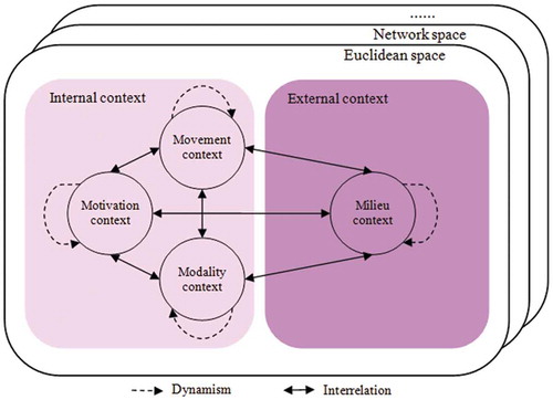
• Motivation context is any propellant and driver that causes movement to take place, such as the reasons and purposes of movement (Bogorny et al. 2014) (e.g., bird seasonal migrations, foraging, breeding), as well as navigation capacity (Nathan et al. 2008) (e.g., tourist intensions of visiting places). Motivation context is dynamic and changeable due to several circumstances during the movement. For example, because of a traffic jam, a driver intends to modify his/her path to the destination.

• Movement context refers to the MPO’s quantitative parameters (e.g., turning angle, speed, acceleration), which are generated as the movement commences. Spaccapietra et al. (2008) termed them movement characteristics, while Dodge, Weibel, and Lautenschütz (2008) called them primary (e.g., speed) and secondary (e.g., acceleration) parameters. Hereinafter, we entitle these dynamic parameters as movement context.

• Modality context is related to the MPO's condition (e.g., physical, psychological), specification (e.g., driver’s experience), and motion capacity (e.g., vehicle type) (Nathan et al. 2008). For example, a tourist’s trajectory could comprise different transportation modes (e.g., bus, taxi, bicycle). Dynamism is a characteristic of modality context.

• Milieu context pertains to any external factor (e.g., weather and climate conditions (Yuan, Wang, and Mitchell 2014; Qiu et al. 2016)) that affects the object’s movement and its internal context positively and/or negatively. For example, heavy rainfall causes the roads to be slippery, which leads to a lower speed of the vehicle. Similar to the previous contexts, the milieu context has a dynamic nature.

All of the earlier contexts are interrelated and affect one another in different manners (the double arrows in Figure 1). As an example, going to work (motivation context) during rush hour (milieu context) causes choosing different transportation modes (modality context), which affects the movement speed (movement context) and travel time.

Object movements and their corresponding contexts are constrained to the spaces that they move through, for example, an automobile to a road, an herbivorous animal to pasture, and an airplane to a specific corridor. Consequently, studying movement is highly dependent on the movement space and its motion capacity. Laube (2009) outlined six basic spaces that accompany point movements: Euclidean homogeneous space, constrained Euclidean space, space–time aquarium, heterogeneous field space, irregular tessellation, and network space. All of the aforementioned 4M contexts, as illustrated in Figure 1, are constrained and are subjected to one of these spaces, and thus, they are modeled differently.

4. Contextualizing the similarity measure

Movements of objects take place for various reasons and under different conditions. This arrangement results directly in diverse movement behaviors and influences the ways that objects interact with one another and the environment. We called these specifications context in Section 3. Therefore, as long as the movements of objects have identical contexts, they express similarity in their trajectories. This relationship persuaded us to analyze the similarity of trajectories with respect to their context. To measure the multidimensional similarity between trajectories based on contextual information, we generalized the classic DTW method and called it CDTW. CDTW allows elements that have similar contexts to be matched even if they are out of phase in the time axis, as described in the following.

Given two trajectories and , it is possible that each element of any trajectory be annotated by dimension(s). We refer to the aforementioned 4M contexts () (cf. Section 3), where for the sake of simplicity, they are labeled , respectively. Therefore, and . Prior to any similarity computation, the trajectory values are normalized to the scale of 1 to be invariant to the amplitude of the scale as well as ease the manipulation, interpretation, and visualization of the results. A five-step procedure describes how to measure the CDTW distance between a pair of trajectories. First, for two trajectories, and , of lengths and , respectively, an empty matrix (M) of size -by- is generated. Second, from the lower left cell of () to the upper right cell of (), the local distance between the trajectory elements is calculated either by the Minkowski distance/-Norm family (i.e., Manhattan distance () or Euclidean distance () by (Equation (1)) or the squared Euclidean distance,

(1)

where and By filling the whole matrix, several paths from to , known as warping paths, can be generated. Each warping path aligns and such that all of the elements match to at least one element of the other trajectory. Accordingly, the global distance between the trajectories and is a cumulative value () of the summation of the warping path values, as calculated by Equation (2).

(2)

, however, is not necessarily the optimum distance between these two trajectories. To determine the optimal path (i.e., the CDTW distance), in the third step, dynamic programming is implemented on matrix as follows: ,

(3)

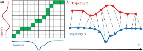
where is the empty trajectory. The results of the previous equations are imported into a new matrix, called the CDTW matrix. Upon completion of this matrix, the optimum warping path can be recovered (i.e., the minimum cumulative value) from to , recursively (see Figure 2a). Fourth, the best CDTW distance between two trajectories and is the upper right cell value of the CDTW matrix. Because the interval or ratio scale types of data are normally used by CDTW method, the magnitudes of the variations are considered in the final distance. Therefore, the earlier equations declare that the CDTW distance for one pair of trajectories is calculated based on the context distance of each element of the first trajectory to the other elements of the second trajectory (see Figure 2b).

Figure 2. (a) Elastic matching achieved by CDTW; (b) trajectory alignments.

While measuring the similarities of the trajectories in different applications, the importance of one dimension could be higher than the others. For example, studying vehicles' movements in the network space at the spatiotemporal dimension (movement context) is more interesting than the drivers’ intensions for movement (motivation context). In contrast, studying birds’ movements in Euclidean spaces is more attractive when concentrating on the reasons for the migration, for example, breeding or foraging (motivation context), compared with studying their speeds (movement context). In this regard, for the fifth step, the related weight of each context () is multiplied by the CDTW distance, where (Equation (4)). The value 0 indicates no weights or no presence of context, and the value 1 denotes the maximum weight of that context. The weight values are application-dependent and can be acquired from different sources, such as optimization techniques, experts’ knowledge, and completing questionnaires, to name a few. Ultimately, is the relative similarity of trajectories and .

(4)

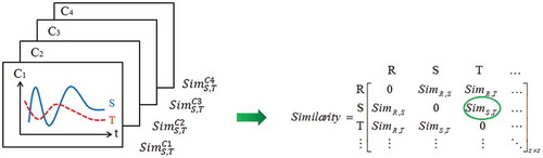
The output of the CDTW is a similarity matrix, which is composed of a series of elements that display the relative similarities of all of the trajectories in terms of all of the 4M contexts (see Figure 3). The similarity matrix is a squared symmetric matrix whose dimension depends on the number of trajectories (). Algorithm 1 provides the pseudo-code of the CDTW approach. The computational time of CDTW is which directly relates to the lengths of the trajectories.

Table

Algorithm 1. CDTW.

Inputs:

two trajectories S and T of size n and m, each element is labeled with four contexts {C1,C2,C3,C4}

W[]: weights

Outputs:

Sim: similarity between S and T

Algorithm:

1.  Sim← 0

2.  For index on contexts k = 1 to 4 do

3.   Compute matrix d(n × m) as distance between S and T on context k

4.   For index on S elements i = 1 to n do

5.    For index on T elements j = 1 to m do

6.     Find minimum of CDTW(si,tj-1), CDTW(si-1,tj), CDTW(si-1,tj-1) as MIN

7.     CDTW(si,tj) = d(si,tj) + MIN

8.    End For

9.   End For

10.   Sim ← Sim + CDTW(si,tj) * Wk

11.  End For

12.  Return Sim

Figure 3. Relative similarity measure of the trajectories.

5. Analyses and results

To evaluate the applicability of our proposed method, CDTW is applied on a real commercial airplane dataset (FlightAware 2016) that considers the 4M contexts. Studying airplane movements and measuring their trajectory similarities in different contexts not only enables the extraction of movement–behavior patterns of airplanes but also helps the decision makers in better planning of the flights and predicting their trajectories according to the contexts (Hurter et al. 2014). In this regard, a number of experiments are conducted that cover a multitude of objectives (Table 1).

Table 1. Overview of the experiments.

Experiment	Context type used	Objective
#1		Exploring the deviations of trajectories from the airway
#2	Motivation, Movement, Milieu	Exploring the relations in contexts
#3	Movement, Modality, Milieu	Incorporating internal and external contexts in similarity measures of trajectories
#4	Motivation, Movement, Modality, Milieu (4M)	Discovering patterns based on the underlying similarities in contexts

5.1. Data

The underlying movement space of commercial airplanes is a constrained Euclidean space, where the airplanes fly through predefined routes that are termed airways. An airway connects two locations and is defined with segments within a specific altitude and corridor width and between fixed geographic coordinates, called waypoints. In this case study, an airway is chosen from the eastern part of the United States of America, between the Orlando International Airport in Orlando, Florida (ICAO code: KMCO), and the John F. Kennedy International Airport in New York City, New York (ICAO code: KJFK), as depicted in Figure 4. The reasons for this selection are due to (1) the location of this airway near the Atlantic Ocean coast, which has a variety of weather conditions; (2) the movement from the south to north direction, which passes a number of geographical latitudes; and (3) the variety of airplane types (i.e., Airbus, Boeing, McDonnell Douglas, and Embraer) and the number of flights per day.

Figure 4. The study area between KMCO and KJFK airports (FlightAware 2016).

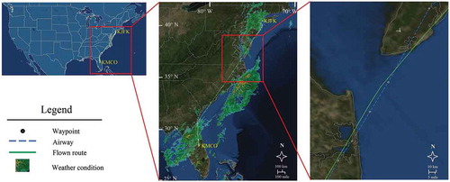
The dataset contains 324 trajectories of real commercial airplanes (FlightAware 2016), which are composed of 51,154 sampling points, as well as the weather conditions (Aviation Weather Center 2016) along the airways. The units for distance, altitude, time, and speed are nautical miles (NM), feet (ft), minutes (min), and knots (Kt), respectively. The angles are measured in a clockwise direction relative to North in degrees. The temporal resolution of the flight data is approximately 1 min, while for the aviation weather data is approximately 1 h. These data are classified into the 4M contexts as outlined in Table 2. Because the meteorological data are obtained from the National Oceanic and Atmospheric Administration on a regular basis, little noise exists in the dataset, and no preprocessing is required. However, outlier detection is applied for airplane trajectories prior to any implementation.

Table 2. Constituent contexts used in trajectory analysis.

Internal context			External context
Motivation context	Movement context	Modality context	Milieu context
-Pilot’s decision	-Airplane instantaneous ground speed -Airplane heading	-Airplane model	-Instantaneous wind speed -Wind direction

5.2. Experiment #1: exploring the deviations of trajectories from the airway

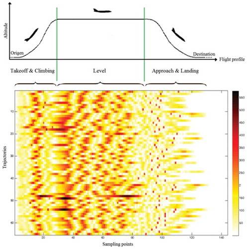
Airplane movement is highly affected by the milieu context, such as the weather conditions and air traffic. This arrangement causes the airplane to deviate from the airway, while still in compliance with the designated air corridor. The objective of this experiment is to quantify the spatial deviation of airplanes trajectories (flown routes) from the designated airways (planned routes). To accomplish this goal, CDTW is implemented on the commercial airplanes dataset to measure the similarity of each trajectory with the airway. More specifically, CDTW enables calculating the spatial deflection of a single element of each trajectory with the corresponding waypoints. Figure 5 provides a visual impression of the deviation magnitudes of each sampling point from the waypoint in colors for 65 sample trajectories at three flight phases: (1) takeoff and climbing (ascending), (2) level (cruise), and (3) approaching and landing (descending).

Figure 5. Spatial deviation of 65 sample airplane trajectories (flown routes) from the airway (planned route).

To quantify the deviation variations of airplane trajectories that correspond to the three flight phases, the (5%, 95%) ranges of the averaged measured distances between the flown routes and airways (planned routes) are calculated in Table 3. Such analysis implies that, for example, for the pair (103.41, 169.33), only 5% of the distances (mismatches) between airplane trajectories and airways are less than 103.41, whereas 95% of them are lesser than 169.33. Subsequently, by exploring the (5%, 95%) ranges, it is feasible to determine any probable outlier that is in the dataset.

Table 3. Average spatial deviation of all of the trajectories from the airways compared with two examples.

Flight phases	(5%, 95%)	S1	S2	S3	T1	T2	T3
Takeoff and climbing	(99.34, 142.45)	171.89			191.96
Level	(150.96, 273.21)		153.06			334.82
Approaching and landing	(59.78, 92.56)			65.42			86.30
Whole flight	(103.41, 169.33)	130.19			204.25

Given two sample trajectories and of lengths and , respectively, both are segmented into three sub-trajectories, namely the takeoff and climbing, level, and approaching and landing phases: [,] and [,]. The (5%, 95%) spatial deviation ranges of these sub-trajectories are calculated in Table 3. It is straightforward to identify the far-off sub-trajectories by comparing their average deviation value with all of the other sub-trajectories as references. For example, on the one hand, the distance value of S₁ = 171.89 (marked bold) is larger than 95% of the average distances for the takeoff and climbing sub-trajectories (142.45), while the distance value of S₃ = 65.42 is smaller than 5% of the average distances of the approaching and landing sub-trajectories (92.56). Consequently, considering the whole deviations of the three phases, trajectory falls into the reference range of (5%, 95%) (130.19) and labels as clear. On the other hand, the 95% average deviation values of both sub-trajectories and deviate from the reference range (marked bold), which results in a larger distance value of the whole trajectory compared to the reference range (204.25 vs. 169.33). Therefore, trajectory is labeled as an outlier and is removed from the dataset.

As the depiction in Figure 5 and the numerical values in Table 3 reveal, the highest to the lowest deviations of the trajectories from the airway are in the level, takeoff and climbing, and approaching and landing phases, respectively. Some studies have contended that such a deviation is dependent on the milieu and motivation contexts (Hurter et al. 2014); thus, they will be investigated in the next experiment.

5.3. Experiment #2: exploring the relations in contexts

The milieu context (e.g., weather conditions) plays a pivotal role in the accurate planning of airplane routes and flight schedules. In this context, wind speed and wind direction are the most prominent meteorological factors that influence airplane movements in all of the aforementioned three flight phases (cf. Section 5.2). A number of studies have been conducted for clustering airplane trajectories (Gariel, Srivastava, and Feron 2011), extracting wind parameters from airplanes movement data (Hurter et al. 2014), and predicting airplane trajectories (Lymperopoulos and Lygeros 2010); however, exploring the interaction of airplane movements with meteorological data has received less attention in movement studies, thus far.

In this experiment, first, the correlation between the spatial deviation of the airplane trajectories from the airway () and the magnitude of the wind speed and wind direction are calculated. Such analysis determines the degree of linear dependency between these two variables. The calculated correlation coefficient of and () implies that partial positive linear dependency exists between the airplane deviations and the wind blow variables. The scatter plot of this implementation is depicted in Figure 6a, where the x-axis shows the wind magnitude and the y-axis shows the airplane deviations from the airways. This arrangement can be justified by the results of the (5%, 95%) range of the level phase (Table 3) in Experiment #1.

Figure 6. Scatter plot shows the correlation and the degree of linear relationship between (a) airplane deviations and wind blowing; (b) flight duration and wind blowing; and (c) approaching operation and wind blowing.

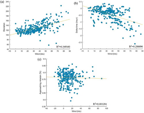
Second, the difference between the scheduled and flown flight durations () is calculated for each trajectory. Thereafter, the correlation coefficient is calculated for as well as the wind speed and wind direction (). Such a value implies a partial negative linear relationship between these two variables and indicates that the more tailwinds there are, the smaller the flight duration is, and vice versa. Such a spatiotemporal similarity search of trajectories can be used to approximate the flight duration and arrival time estimation with respect to the wind parameters. The scatter plot in Figure 6b illustrates the wind magnitude on the x-axis and the time difference on the y-axis.

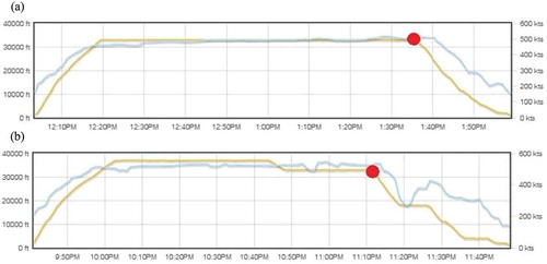
Pilots normally use two approaching techniques prior to landing: continuous descent final approach (CDFA) and dive-and-drive. The former is a procedure with a constant descent of the airplane’s altitude, without any level off (Figure 7a). In the latter, the altitude of the airplane decreases in a stepwise manner (descent and level) until the airplane lands (Figure 7b) (Federal Aviation Administration Advisory Circular 120-108 2011). As the airplane travels longer distances in the third phase of the flights through the dive-and-drive technique, pilots normally commence the approaching operation earlier in comparison to the CDFA technique (the red dots in Figure 7), in other words, after traversing approximately 70% and 80% of the flight passes for the dive-and-drive and CDFA techniques, respectively. At the same time, as can be seen from the speed profile in Figure 7a, the airplane speed decreases at a constant rate from approaching to landing in the CDFA technique, while for the dive-and-drive technique, the airplane speed variation occurs in the third phase of the speed profile (Figure 7b). Thus, the different approaching techniques directly affect the geometries of the trajectories and their speed profiles, which results in the diversity of trajectory similarity values. Choosing either of these approaching techniques is highly related to the pilot’s experience in riding the airplane (motivation context), the availability of instruments in the airplane and the equipment of the airport (modality context), and in some circumstances, to the weather conditions (milieu context). As the third examination, the correlation coefficient between the approaching operation starting time and the magnitude of the wind speed and wind direction are calculated only on the third phase of the flights (approaching and landing sub-trajectories) as . This value and the scatter plot in Figure 6c imply no relationship between these two variables in our dataset.

Figure 7. Approaching techniques: (a) CDFA; (b) Dive-and-dive (Altitude (ft.) in orange line, speed (Kts) in blue line, and beginning of approaching operation in red dot) (FlightAware 2016). For full colour versions of the figures in this paper, please see the online version.

5.4. Experiment #3: incorporating internal and external contexts in the similarity measure of the trajectories

This experiment attempted to determine the role of the internal and external contexts in similarity measures of trajectories. To accomplish this goal, CDTW is applied to the segmented flight trajectories (i.e., takeoff and climbing, level, and approaching and landing phases) as well as to the whole flight trajectory (all of the three phases together) while taking the contextual information into account. The similarities of these (sub-)trajectories are assessed from two main perspectives, as follows.

From the first perspective (P1), there are considerable variations in the movement contexts of airplanes (i.e., airplane speed and heading) and the number of modality contexts (i.e., airplane model), which could affect the similarity results of the (sub-)trajectories. More specifically, we believe that employing airplane ground speeds (i.e., the rate of alteration in positions), headings (i.e., directions of movements), and their models accompanying the spatial dimensions of the airplanes reflect the similarities of trajectories more realistically. This information (except for the airplane models) can be represented as profiles over time (cf. Figure 2b). For generating the directionality component (e.g., heading) profile, we exploit the azimuth (Az) of each airplane over the course of time. For this purpose and to preserve the relative distances between the directions, we considered 0°–180° for the first and second quarter angles and Az-360° for the third and fourth quarter angles. Then, the distance between two angles is calculated by the absolute difference in these two values. For example, the distance between the N30E (30°) and N45W (315°) directions is |30°− (315° − 360°)| = 75°. To apply the airplane types in the computation of the similarity measure, we consider 0 and 1 values (hereinafter called the modality distance) to be implemented into the similarity results of the trajectories for identical and different airplane types, respectively. For example, if both trajectories are generated from Boeing airplanes, then their modality distance is 0, while if one of them is generated by an Airbus airplane, then the value 1 is added as the modality distance in the similarity process. Second, some of the variations in airplane movements are due to the milieu context. Therefore, as the second perspective (P2), we believe that the atmospheric conditions (i.e., wind direction and magnitude) should be coupled with the similarity results of P1. In other words, the airplane movement, to a considerable extent, is affected by the wind direction and magnitude during the flight; thus, both of these should be considered as indicators for finding commonalities in the trajectories. The different settings of P1 and P2 are as follows:

Perspective 1: A: Latitude – Longitude

B: Altitude

C: Airplane speed

D: Airplane heading

E: Latitude – Longitude – Altitude

F: Latitude – Longitude – Altitude – Airplane model

G: Latitude – Longitude – Altitude – Airplane model – Airplane speed and heading

Perspective 2:H: Wind speed

I: Wind direction

J: Latitude – Longitude – Altitude – Airplane model – Airplane speed and heading – Wind speed and direction

The relative CDTW distances of 324 (sub-)trajectories for individuals and combinations of the aforementioned parameters are computed and statistically analyzed by their means and standard deviations in Table 4. In addition, the CDTW distances along with their probability distributions are illustrated for all of the phases in Figure 8. From P1, the average similarity measure and the related standard deviation of whole trajectories at spatial dimension (two-dimensional [2D]) compared to other similarity values is very high (A4: 12.676 ± 10.158/black line in Figure 8d). At the same time, the average similarity distance of the airplanes’ altitudes at the level phase is high (B2: 17.450 ± 17.628), which is mainly due to the differences in the flight altitudes (which range from 33,000 to 39,000 ft). This value, however, dramatically drops for the whole trajectory (B4: 0.033 ± 0.034) when exploiting other flight phase values, B1 and B3. Consequently, the average similarity distance of the airplanes’ altitudes significantly reduces the average similarity distance of the trajectories from 2D (A4: 12.676 ± 10.158/black line in Figure 8d) to 3D (E4: 6.355 ± 5.078/blue line in Figure 8d) space. When aggregating the airplanes' speeds and headings (movement contexts) to the previous similarity results, the average similarity distance for the trajectories at P1 is reduced again. This finding indicates that airplanes normally follow similar speeds and directions during the flight (G4: 2.925 ± 2.173/green line in Figure 8d).

Table 4. Statistics of (sub-)trajectory similarity measures demonstrating the mean ± standard deviation of single variables and combinations of context variable(s).

Perspective		1. Takeoff and climbing phase	2. Level phase	3. Approaching and landing phase	4. Whole flight
P1	A	5.000 ± 5.047	11.069 ± 8.750	8.219 ± 6.59	12.676 ± 10.158
	B	0.012 ± 0.006	17.450 ± 17.628	0.015 ± 0.01	0.033 ± 0.034
	C	0.587 ± 0.772	0.348 ± 0.405	0.759 ± 1.017	1.584 ± 1.369
	D	0.060 ± 0.049	5.736 ± 5.218	0.074 ± 0.064	0.322 ± 0.267
	E	2.506 ± 2.524	14.260 ± 9.883	4.117 ± 3.295	6.355 ± 5.078
	F	1.673 ± 1.683	9.501 ± 6.589	2.877 ± 2.532	4.237 ± 3.385
	G	1.133 ± 1.073	6.921 ± 4.133	1.893 ± 1.634	2.925 ± 2.173
P2	H	2.268 ± 4.516	10.812 ± 12.495	3.249 ± 10.147	3.911 ± 3.175
	I	3.381 ± 4.242	3.937 ± 5.886	4.543 ± 5.390	11.643 ± 10.831
	J	1.617 ± 1.273	7.051 ± 3.662	2.465 ± 2.150	4.310 ± 2.549

Figure 8. Similarity distribution values of sub-trajectories and trajectories in different contexts: (a) Takeoff and climbing phase; (b) Level phase; (c) Approaching and landing phase; (d) Whole flight.

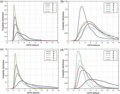
From P2, we assessed the impact of the milieu context by incorporating the wind speed and the direction values in the similarity measure process. As seen in cell H2 of Table 4, there is a significant variation in the wind speed in the second (level) phase of the flights (H2: 10.812 ± 12.495), which implies a positive relation between the altitude and wind speed. Similarly, there is a significant variation in the wind direction across the study area (I4: 11.643 ± 10.831). By integration of the wind speed and wind direction parameters (H and I) into the similarity results of P1, this value slightly increases to 4.310 ± 2.549 for whole trajectories (J4/red line in Figure 8d).

The weight parameter () characterizes the presence and degree of importance for each context. Defining such a parameter, however, is highly application dependent and is determined based on practical needs. In the following, we intend to explore the effects of context weights on similarity measure results of trajectories. To accomplish this goal, we consider different weights for each comparative component (i.e., spatial dimension, internal context, and external context), which results in varied similarity values (see Table 5). More specifically, seven settings of weights (W1–W7) are introduced, and the CDTW method is applied to measure the corresponding distances. The first two results (marked bold) refer to the traditional DTW distance because it computes the distances between the trajectories only at the spatial dimension. The next five results arrange the spatial and context variables together: W3 and W4 (spatial and internal context), W5 and W6 (spatial and external context), and W7 (spatial, internal context, and external context). Such multiplicative weights are defined to be between 0 and 1. The weight of zero implies no context, and the weight coefficient ½ implies a higher importance than the weight coefficient of ¼. These numbers are chosen as representative values of weights, only to demonstrate the capability and sensitivity of CDTW in handling weights as well as to represent how weighting can influence the similarity results.

Table 5. Statistics of the weighted similarity measures of trajectories demonstrating mean ± standard deviation of single variables and combinations of context variables.

	Spatial dimension		Internal context		External context
Weight	Latitude – Longitude	Altitude	Airplane speed	Airplane heading	Wind speed	Wind direction	∑	CDTW distance (mean ± SD)
W1	1	0	0	0	0	0	1	12.676 ± 10.158
W2	1/2	1/2	0	0	0	0	1	6.355 ± 5.078
W3	1/4	1/4	1/2	0	0	0	1	5.816 ± 3.437
W4	1/4	1/4	1/4	1/4	0	0	1	3.144 ± 2.598
W5	1/4	1/4	0	0	1/2	0	1	5.365 ± 3.002
W6	1/4	1/4	0	0	1/4	1/4	1	7.288 ± 3.459
W7	1/6	1/6	1/6	1/6	1/6	1/6	1	5.506 ± 2.613

As the results in Table 6 show, the average spatial distance at two dimensions (latitude and longitude) has the highest value (12.676), whereas this value decreases to almost half (6.355) when the third spatial dimension (i.e., the altitude) is incorporated into the computation. There might be an interest in exploring the role of the weighted internal and external context components, both individually and collaboratively. For this purpose, we individually examined the average similarity result of the airplane speed and wind speed in W3 and W5, respectively, as well as the airplane speed and heading in W4 and the wind speed and direction in W6, collaboratively. Placing the spatial dimension and both the weighted internal and external contexts together, the average CDTW distance becomes 5.506 for all of the ingredients. This practice shows how CDTW can be applied to measure the similarities of trajectories while taking into account a variety of both spatial and contextual weights in separate and combinatorial forms.

Table 6. Pattern discovery based on underlying contexts.

Test	Pattern	Objective	Result
1	(a) Latitude – Longitude – Altitude	Discovering sub-trajectories used CDFA technique	87 out of 324
	(b) Latitude – Longitude – Altitude	Discovering sub-trajectories used dive-and-drive technique	207 out of 324
2	(c) Latitude – Longitude – Airplane speed	Discovering speed profiles of CDFA technique	81 out of 324
	(d) Latitude – Longitude – Airplane speed	Discovering speed profiles of dive-and-drive technique	198 out of 324
3	(e) Latitude – Longitude – Altitude	Distinguishing Boeing trajectories	35 out of 44
	(f) Latitude – Longitude – Altitude	Distinguishing Airbus trajectories	177 out of 218
	(g) Latitude – Longitude – Altitude	Distinguishing McDonnell Douglas trajectories	37 out of 44
	(h) Latitude – Longitude – Altitude	Distinguishing Embraer trajectories	13 out of 18
4	(i) Latitude – Longitude – Altitude	Discovering spatial patterns	206 out of 324
	(j) Airplane speed and heading	Discovering patterns based on movement context	254 out of 324
	(k) Wind speed and direction	Discovering patterns based on milieu context	136 out of 324
	(l) Latitude – Longitude – Altitude – Wind speed – Wind direction	Discovering patterns based on spatial information and milieu context	193 out of 324
	(m) Latitude – Longitude – Altitude – Airplane speed and heading – Wind speed and direction	Discovering patterns based on spatial information, movement context, and milieu context	175 out of 324

5.5. Experiment #4: discovering patterns based on the underlying similarities in contexts

The results of similarity measures can be exploited in trajectory classification (Dodge, Weibel, and Forootan 2009), trajectory clustering (Izakian, Mesgari, and Abraham 2016), and pattern discovery (Guo et al. 2012). The phrase pattern discovery is denoted as “fitting a model to data, revealing structures, or inferring high-level delineation from the dataset” (Fayyad, Piatetsky-Shapiro, and Smyth 1996). The progress of discovering patterns from the trajectories at spatial and spatiotemporal levels (Laube 2009) affirms its importance in movement analysis. According to related research on pattern mining of MPOs, Dodge, Weibel, and Laube (2011) used the Euclidean distance approach for a similarity measure of trajectories while aiming to find the so-called coincidence (spatiotemporal) and concurrence (movement parameters) patterns of North Atlantic hurricanes. From the methodological standpoint, the employed Euclidean distance is a very brittle distance measure because it can be applied only to trajectories of the same size. Therefore, a robust alternative method that is capable of accommodating trajectories that have different sizes is crucial. From a dimensional perspective, the previous study covers only the space, time, and movement parameters in pattern mining. These dimensions are more or less fit into our movement context class, while other contexts are neglected.

To the best of our knowledge, no research has been conducted on pattern mining of multisize trajectories based on similarity measures and contextual information. This experiment, therefore, intends to discover the most prominent patterns among the commercial airplane trajectories with respect to the commonalities in their contexts. Our proposed CDTW approach not only allows trajectories of different sizes to be compared but also incorporates multiple contexts in pattern discovery.

First, we exploit the results of Experiment #3, where the CDTW approach is applied to the dataset for calculating the context distances (similarities) of trajectories. Second, it is required to define a reference range in which the trajectories that fit into it will share identical patterns. Normally, such ranges are distinguished by thresholds (). Dodge, Weibel, and Laube (2011) defined a fixed-value threshold for different types of variables based on trial and error, while we believe that contexts should have their own thresholds with respect to their natures. Thus, we calculate the matching thresholds as one-quarter of the maximum standard deviation of the trajectory similarities in each context, which is also confirmed by Chen, Özsu, and Oria (2005). However, larger thresholds can be set if large variations in the probability values (cf. Figure 6) are expected (Coro, Pagano, and Ellenbroek 2014). Third, a reference trajectory is selected: the trajectory that has the least deviation from the airway and the minimum difference between the scheduled and flown flight durations. Consequently, trajectories for which their context distances are equal and/or smaller than fit into the reference range and demonstrate similar patterns.

We conduct a number of tests, as demonstrated in Table 6, to discover multidimensional patterns in the dataset and to assess the role of contextual information in pattern discovery. Test #1 is dedicated to the motivation context, where pilots normally use two approaching techniques – CDFA and dive-and-drive – prior to landing (cf. Experiment #2). It is desired to discover such patterns and to determine which pattern is most often used by pilots. Figure 9a and b, respectively, illustrates the discovered sub-trajectories (of the third phase) with identical patterns (in green) based on the reference patterns (in red) for the CDFA and the dive-and-drive techniques. We found that 64% of trajectories follow the dive-and-drive technique, and 27% of them follow the CDFA technique. The remaining 9% sub-trajectories do not fall into either of these techniques.

Figure 9. Discovered pattern (in green) based on the reference trajectory (in red): (a) CDFA spatial pattern of the third phase of the flight; (b) Dive-and-drive spatial pattern of the third phase of the flight; (c) CDFA speed pattern; (d) Dive-and-drive speed pattern; (e) Boeing pattern; (f) Airbus pattern; (g) McDonnell Douglas pattern; (h) Embraer pattern.

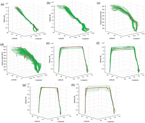
As previously mentioned in Experiment #2, the airplane speed profiles have significant alterations in the third phase of the flights when pilots are using the dive-and-drive technique, while for the CDFA technique, they have smooth decent trends. In this regard, Test #2 is dedicated to discovering the trajectories that show identical patterns in terms of their speed profiles (i.e., movement context). Figure 9c and d depicts the discovered similar speed profiles (in green) based on the reference patterns (in red) for CDFA and the dive-and-drive techniques, respectively. It is revealed that 61% of the trajectories have significant variations in their speed profiles at the approaching and landing phase. This finding justifies the findings in Test #1 to almost 95%. In addition, 25% of the speed profiles follow the reference pattern of the CDFA technique. The remaining 14% of speed profiles do not fall into either of these techniques.

We evaluate the applicability of CDTW through finding identical patterns of four airplane models (i.e., modality context) in Test #3. To accomplish this goal, one reference trajectory is selected for each model, and the corresponding patterns are extracted. Figure 9e–h illustrates these patterns for Boeing, Airbus, McDonnell Douglas, and Embraer, respectively. The computed counts of these trajectories are summarized in Table 6.

It is feasible to investigate the role of internal and external contextual information in discovering patterns individually and collaboratively. For this purpose, Test #4 was conducted, and five settings of spatial and contextual information are defined in Table 6. For the single context assessment, the first setting (i) discovers the traditional spatial pattern of 324 trajectories in three dimensions. The second (j) and third (k) settings are dedicated to the patterns of movement context (i.e., airplane speed and heading) and the milieu context (i.e., wind speed and direction) variables, respectively. The results of these implementations demonstrate a large variation in the number of discovered trajectories despite the fact that their reference trajectory is the same. For the combinational context assessment, the fourth setting (l) discovers the patterns of airplane movements and the wind speeds and directions along the flights. This test is useful for identifying the airplanes that have the most stable conditions in different atmospheric conditions. The outcome suggests that 193 distinguished trajectories share tailwind conditions and are more similar than the trajectories that face crosswinds or headwinds. Additionally, the Airbus trajectories are the stabilized trajectories in this test because they have the least distances to the reference pattern. Finally, setting (m) puts all of the spatial, internal, and external contextual information together and discovers 175 similar trajectories. Although the number of discovered trajectories is lower than the previous implementations (e.g., i and l), this approach demonstrates the actual similar trajectories in terms of the spatial and contextual information.

6. Discussion

As presented in Section 5, the CDTW method is capable of accomplishing similarity measurement of trajectories and discovering their inherent patterns based on their underlying contexts. In this section, we discuss the main findings and achievements from methodological and experimental perspectives.

From the methodological standpoint, the CDTW method is applicable for quantifying the relative similarities between trajectories based on their underlying 4M contexts. The classic DTW, in essence, was represented as a one-dimensional (spatial) method in movement analysis. However, in this article, the CDTW method is utilized to analyze a variety of internal and external contexts, both individually and collaboratively. In other words, CDTW can be applied to any spatial and contextual information that can be represented as sequences along the time axis, such as speed, position, or direction, to name a few. This capability can be specifically seen from the similarity results in Experiment #3. Furthermore, CDTW improves upon the traditional DTW in which the context weights can be considered in similarity searches. The presence and degree of importance of each context are controlled by the weight parameter (). However, defining such a parameter is highly application-dependent and is determined based on practical needs. It is also shown that CDTW is a robust method for discovering multidimensional contextual patterns among the trajectories and sub-trajectories of unequal sizes and sampling rates in Experiment #4. For example, the average accuracy of CDTW in distinguishing airplane models is almost 80%. Nevertheless, CDTW is functional where time is not a major component to be investigated because it performs based on elastic shifting of the time axis.

What is noticeable about this study area is the underlying movement space in which the airplanes fly, which is known as constrained Euclidean space. The predefined airways and air corridors are the main features of this space that limit the airplane movements. Compared to homogeneous Euclidean space, movement variation in constrained Euclidean space is trivially much lower. CDTW is shown to be a robust method that is sensitive to small alterations and abrupt changes in the study area; some examples include the spatial distances of airplane deviations from the airways (Experiment #1), the similarity results of airplane speeds and directions in the three flight phases, and the effects of the wind speed and direction on the ultimate similarity measures (Experiment #3, Table 4), as well as discovering movement patterns (Experiment #4).

From an experimental perspective, it is revealed that the milieu context can be treated as a remarkable factor for the deviations of airplanes from the airways (cf. Experiment #1). Pilots are obliged to touch the airway, but the presence of strong crosswinds and their influence on the airplanes’ movements leads to maneuvers in the air corridor, either intentional or unintentional. The deviation–wind correlation calculation in Experiment #2 justifies the association between the movement and milieu context. Moreover, the high context distance of the wind speed profiles in Experiment #2 (Table 4) forcefully implies a correlation between altitude and wind speed; in other words, the higher the altitude is, the greater the wind speed will be, which is also confirmed by Park and Jang (2016). By the same token, wind speeds and directions along the flights significantly affect the similarity results of the trajectories. Moreover, the pilot’s decision (the motivation context) in choosing either the CDFA or the dive-and-drive techniques at the third phase of the flight (approaching and landing) is a pivotal factor for the spatial mismatches between the flown routes and planned routes. This issue is analyzed in Experiment #4, where 64% of the pilots used the dive-and-drive technique, and 27% of them used the CDFA technique.

Additionally, the wind directly affects the flight duration with regard to its direction and magnitude. Tailwinds blowing in the direction of the flight speed up the airplanes and consequently decrease the flight durations. In contrast, headwinds blowing against the flight direction slow down airplane speeds and increase flight durations. The time–wind correlation calculation in Experiment #2 again justifies the association between movement and the milieu context.

7. Conclusions and future work

In this article, we provided new insights into the similarity analysis and pattern discovery of trajectories based on spatial and contextual information. Specifically, we proposed a taxonomy for contexts in movement studies in light of internal states and external factors, namely motivation, movement, modality, and milieu contexts. Thereafter, we developed the CDTW method for assessing the similarities of trajectories, by including not only their spatial footprints but also a notion of the above 4M contexts. The effectiveness of CDTW method is examined in several experiments on the commercial airplanes dataset. The results demonstrated that CDTW method can be successfully applied in similarity analysis of trajectories and can help to provide pattern discovery in large datasets. Furthermore, the results underpin the fact that movement is highly affected by these 4M contexts in both positive and negative manners. Compared to the closely related work by Buchin, Dodge, and Speckmann (2014), this research provides advances that are mainly from (1) imposing motivation and modality contexts besides movement and milieu contexts in the similarity analysis of trajectories, (2) using a robust distance measure that is sensitive to small alterations in contexts in a constrained Euclidean space, and (3) discovering patterns with respect to the underlying 4M contexts.

There are multiple directions toward extending this research and future work. We will further employ the CDTW method in more case studies (e.g., human, animal movements), in particular accounting different forms of 4M contexts (e.g., traffic, land cover, user’s profile), and will assess the effectiveness of CDTW method in other movement spaces. Moreover, we plan to apply the 4M contexts into other time series and computational geometry methods aiming to quantify the similarity of trajectories based on spatial, temporal, and contextual dimensions. Another promising future work relates to enriching qualitative (topological) methods with contextual information to investigate movement behaviors. Furthermore, we are interested in incorporating the 4M context types into other geographic knowledge discovery issues, including trajectory segmentation, classification, and clustering. Finally, there is an enormous potential to exploring the interaction (i.e., attraction or avoidance) of MPOs with each other and with the other proposed 4M contexts.

Disclosure statement

No potential conflict of interest was reported by the authors.

References

- Ahearn, S. C., S. Dodge, A. Simcharoen, G. Xavier, and J. L. D. Smith. 2016. “A Context-Sensitive Correlated Random Walk: A New Simulation Model for Movement.” International Journal of Geographical Information Science 1–17. doi:10.1080/13658816.2016.1224887.
- Andrienko, G., N. Andrienko, and M. Heurich. 2011. “An Event-Based Conceptual Model for Context-Aware Movement Analysis.” International Journal of Geographical Information Science 25: 1347–1370. doi:10.1080/13658816.2011.556120.
- Aviation Weather Center. 2016. Accessed 10 December 2016. www.aviationweather.gov.
- Berndt, D. J., and J. Clifford. 1994. “Using Dynamic Time Warping to Find Patterns in Time Series.” KDD Workshop, Seattle, WA, 24 April 1994 359–370.
- Bogorny, V., C. Renso, A. R. De Aquino, F. De Lucca Siqueira, and L. O. Alvares. 2014. “CONSTAnT – A Conceptual Data Model for Semantic Trajectories of Moving Objects.” Transactions in GIS 18: 66–88. doi:10.1111/tgis.2014.18.issue-1.
- Bruderlin, A., and L. Williams. 1995. “Motion Signal Processing.” Proceedings of the 22nd Annual Conference on Computer Graphics and Interactive Techniques, (SIGGRAPH '95), Susan G. Mair and Robert Cook (Eds.) ACM, New York, NY. 97-104. doi: 10.1145/218380.218421.
- Buchin, K., M. Buchin, J. Gudmundsson, M. Löffler, and J. Luo. 2011. “Detecting Commuting Patterns by Clustering Subtrajectories.” International Journal of Computational Geometry & Applications 21: 253–282. doi:10.1142/S0218195911003652.
- Buchin, M., S. Dodge, and B. Speckmann. 2014. “Similarity of Trajectories Taking into Account Geographic Context.” Journal of Spatial Information Science 9: 101–124.
- Chavoshi, S. H., B. De Baets, T. Neutens, H. Ban, O. Ahlqvist, G. De Tré, and N. Van De Weghe. 2014. “Knowledge Discovery in Choreographic Data Using Relative Motion Matrices and Dynamic Time Warping.” Applied Geography 47: 111–124. doi:10.1016/j.apgeog.2013.12.007.
- Chen, L., M. T. Özsu, and V. Oria. 2005. “Robust and Fast Similarity Search for Moving Object Trajectories.” Proceedings of the 2005 ACM SIGMOD International Conference on Management of Data, ACM, Baltimore, MD. 491–502. doi: 10.1145/1066157.1066213.
- Coro, G., P. Pagano, and A. Ellenbroek. 2014. “Comparing Heterogeneous Distribution Maps for Marine Species.” GIScience & Remote Sensing 51: 593–611. doi:10.1080/15481603.2014.959391.
- Demšar, U., K. Buchin, F. Cagnacci, K. Safi, B. Speckmann, N. Van De Weghe, D. Weiskopf, and R. Weibel. 2015. “Analysis and Visualisation of Movement: An Interdisciplinary Review.” Movement Ecology 3: 1–24. doi:10.1186/s40462-015-0032-y.
- Dey, A. K. 2001. “Understanding and Using Context.” Personal Ubiquitous Computing 5: 4–7. doi:10.1007/s007790170019.
- Ding, H., G. Trajcevski, P. Scheuermann, X. Wang, and E. Keogh. 2008. “Querying and Mining of Time Series Data: Experimental Comparison of Representations and Distance Measures.” Proceedings of the VLDB Endowment 1: 1542–1552. doi:10.14778/1454159.
- Dodge, S. 2011. “Exploring Movement Using Similarity Analysis. PhD diss., University of Zurich.
- Dodge, S., G. Bohrer, K. Bildstein, S. C. Davidson, R. Weinzierl, M. J. Bechard, D. Barber, et al. 2014. “Environmental Drivers of Variability in the Movement Ecology of Turkey Vultures (Cathartes Aura) in North and South America.” Philosophical Transactions of the Royal Society B: Biological Sciences 369: 20130195. doi:10.1098/rstb.2013.0195.
- Dodge, S., G. Bohrer, R. Weinzierl, S. C. Davidson, R. Kays, D. Douglas, S. Cruz, J. Han, D. Brandes, and M. Wikelski. 2013. “The Environmental-Data Automated Track Annotation (Env-Data) System: Linking Animal Tracks with Environmental Data.” Movement Ecology 1: 3–14. doi:10.1186/2051-3933-1-3.
- Dodge, S., P. Laube, and R. Weibel. 2012. “Movement Similarity Assessment Using Symbolic Representation of Trajectories.” International Journal of Geographical Information Science 26: 1563–1588. doi:10.1080/13658816.2011.630003.
- Dodge, S., R. Weibel, S. C. Ahearn, M. Buchin, and J. A. Miller. 2016. “Analysis of Movement Data.” International Journal of Geographical Information Science 30: 825–834. doi:10.1080/13658816.2015.1132424.
- Dodge, S., R. Weibel, and E. Forootan. 2009. “Revealing the Physics of Movement: Comparing the Similarity of Movement Characteristics of Different Types of Moving Objects.” Computers, Environment and Urban Systems 33: 419–434. doi:10.1016/j.compenvurbsys.2009.07.008.
- Dodge, S., R. Weibel, and P. Laube. 2011. “Trajectory Similarity Analysis in Movement Parameter Space.” Proceedings of GISRUK, Plymouth, UK, April 27–29.
- Dodge, S., R. Weibel, and A.-K. Lautenschütz. 2008. “Towards a Taxonomy of Movement Patterns.” Information Visualization 7: 240–252. doi:10.1057/palgrave.ivs.9500182.
- Fayyad, U., G. Piatetsky-Shapiro, and P. Smyth. 1996. “From Data Mining to Knowledge Discovery in Databases.” AI Magazine 17: 37.
- Federal Aviation Administration Advisory Circular 120-108. 2011 Accessed 10 December 2016. www.faa.gov/documentLibrary/media/Advisory_Circular/AC%20120-108.pdf.
- FlightAware. 2016. Accessed 10 December 2016. www.flightaware.com.
- Furtado, A. S., D. Kopanaki, L. O. Alvares, and V. Bogorny. 2015. “Multidimensional Similarity Measuring for Semantic Trajectories.” Transactions in GIS. 20: 280-298. doi:10.1111/tgis.issue-2.
- Gariel, M., A. N. Srivastava, and E. Feron. 2011. “Trajectory Clustering and an Application to Airspace Monitoring.” IEEE Transactions on Intelligent Transportation Systems 12: 1511–1524. doi:10.1109/TITS.2011.2160628.
- Ghisu, T., B. Arca, G. Pellizzaro, and P. Duce. 2015. “An Optimal Cellular Automata Algorithm for Simulating Wildfire Spread.” Environmental Modelling & Software 71: 1–14. doi:10.1016/j.envsoft.2015.05.001.
- Gschwend, C. 2015. “Relating Movement to Geographic Context – Effects of Preprocessing, Relation Methods and Scale.” PhD diss., University of Zurich.
- Guo, D., X. Zhu, H. Jin, P. Gao, and C. Andris. 2012. “Discovering Spatial Patterns in Origin-Destination Mobility Data.” Transactions in GIS 16: 411–429. doi:10.1111/tgis.2012.16.issue-3.
- Güting, R. H., and M. Schneider. 2005. Moving Objects Databases. San Francisco, CA:Elsevier.
- Hurter, C., R. Alligier, D. Gianazza, S. Puechmorel, G. Andrienko, and N. Andrienko. 2014. “Wind Parameters Extraction from Aircraft Trajectories.” Computers, Environment and Urban Systems 47: 28–43. doi:10.1016/j.compenvurbsys.2014.01.005.
- Izakian, Z., M. S. Mesgari, and A. Abraham. 2016. “Automated Clustering of Trajectory Data Using a Particle Swarm Optimization.” Computers, Environment and Urban Systems 55: 55–65. doi:10.1016/j.compenvurbsys.2015.10.009.
- Laube, P. 2009. Progress in Movement Pattern Analysis. The Netherlands: IOS Press.
- Laube, P. 2014. Computational Movement Analysis. Cham: Springer International Publishing AG.
- Lin, D. 1998. “An Information-Theoretic Definition of Similarity.” In Proceedings of the Fifteenth International Conference on Machine Learning (ICML '98), Jude W. Shavlik (Ed.). Morgan Kaufmann Publishers Inc., San Francisco, CA, 296–304.
- Little, J. J., and Z. Gu. 2001. “Video Retrieval by Spatial and Temporal Structure of Trajectories.” Proceedings of the SPIE Storage and Retrieval for Media Databases. San Jose, CA, 20 January 2001 545–552.
- Liu, H., and M. Schneider. 2012. “Similarity Measurement of Moving Object Trajectories.” In Proceedings of the Third ACM SIGSPATIAL International Workshop on GeoStreaming. Redondo Beach, CA: ACM.
- Long, J. A., and T. A. Nelson. 2013. “A Review of Quantitative Methods for Movement Data.” International Journal of Geographical Information Science 27: 292–318. doi:10.1080/13658816.2012.682578.
- Lymperopoulos, I., and J. Lygeros. 2010. “Sequential Monte Carlo Methods for Multi-Aircraft Trajectory Prediction in Air Traffic Management.” International Journal of Adaptive Control and Signal Processing 24: 830–849. doi:10.1002/acs.1174.
- Mcintosh, J., and M. Yuan. 2005. “Assessing Similarity of Geographic Processes and Events.” Transactions in GIS 9: 223–245. doi:10.1111/tgis.2005.9.issue-2.
- Nathan, R., W. M. Getz, E. Revilla, M. Holyoak, R. Kadmon, D. Saltz, and P. E. Smouse. 2008. “A Movement Ecology Paradigm for Unifying Organismal Movement Research.” Proceedings of the National Academy of Sciences 105: 19052–19059. doi:10.1073/pnas.0800375105.
- Parent, C., S. Spaccapietra, C. Renso, G. Andrienko, G. Andrienko, V. Bogorny, M. L. Damiani, et al. 2013. “Semantic Trajectories Modeling and Analysis.” ACM Computing Surveys 45: 1–32. doi:10.1145/2501654.2501656.
- Parizeau, M., and R. Plamondon. 1990. “A Comparative Analysis of Regional Correlation, Dynamic Time Warping, and Skeletal Tree Matching for Signature Verification.” IEEE Transactions on Pattern Analysis and Machine Intelligence 12: 710–717. doi:10.1109/34.56215.
- Park, J., and D.-H. Jang. 2016. “Application of MK-PRISM for Interpolation of Wind Speed and Comparison with Co-Kriging in South Korea.” GIScience & Remote Sensing 53: 421–443. doi:10.1080/15481603.2016.1192373.
- Purves, R. S., P. Laube, M. Buchin, and B. Speckmann. 2014. “Moving beyond the Point: An Agenda for Research in Movement Analysis with Real Data.” Computers, Environment and Urban Systems 47: 1–4. doi:10.1016/j.compenvurbsys.2014.06.003.
- Qiu, B., Z. Wang, Z. Tang, Z. Liu, D. Lu, C. Chen, and N. Chen. 2016. “A Multi-Scale Spatiotemporal Modeling Approach to Explore Vegetation Dynamics Patterns under Global Climate Change.” GIScience & Remote Sensing 1–18. doi:10.1109/LGRS.2016.2633622.
- Ranacher, P., and K. Tzavella. 2014. “How to Compare Movement? A Review of Physical Movement Similarity Measures in Geographic Information Science and Beyond.” Cartography and Geographic Information Science 41: 286–307. doi:10.1080/15230406.2014.890071.
- Sakoe, H., and S. Chiba. 1978. “Dynamic Programming Algorithm Optimization for Spoken Word Recognition.” IEEE Transactions on Acoustics, Speech, and Signal Processing 26: 43–49. doi:10.1109/TASSP.1978.1163055.
- Siła-Nowicka, K., J. Vandrol, T. Oshan, J. A. Long, U. Demšar, and A. S. Fotheringham. 2016. “Analysis of Human Mobility Patterns from GPS Trajectories and Contextual Information.” International Journal of Geographical Information Science 30: 881–906. doi:10.1080/13658816.2015.1100731.
- Spaccapietra, S., C. Parent, M. L. Damiani, J. A. De Macedo, F. Porto, and C. Vangenot. 2008. “A Conceptual View on Trajectories.” Data & Knowledge Engineering 65: 126–146. doi:10.1016/j.datak.2007.10.008.
- Spaccapietra, S., C. Parent, and L. Spinsanti. 2013. “Trajectories and Their Representations.” In Mobility Data: Modeling, Management, and Understanding, edited by C. Renso, S. Spaccapietra, and E. Zima´ Nyi. New York, NY: Cambridge University.
- Vahidnia, M. H., and A. A. Alesheikh. 2014. “Plain Move Predicate and Its Consistency Concerning the Moving Agents in a Network.” International Journal of Geographical Information Science 28: 2145–2177. doi:10.1080/13658816.2014.912281.
- Xia, Y., G.-Y. Wang, X. Zhang, G.-B. Kim, and H.-Y. Bae. 2010. “Research of Spatio-Temporal Similarity Measure on Network Constrained Trajectory Data.” In Rough Set and Knowledge Technology: 5th International Conference, RSKT 2010, Beijing, China, October 15–17, 2010, edited by J. Yu, S. Greco, P. Lingras, G. Wang, and A. Skowron. Berlin, Heidelberg: Springer Berlin Heidelberg.
- Xiao, X., Y. Zheng, Q. Luo, and X. Xie. 2014. “Inferring Social Ties between Users with Human Location History.” Journal of Ambient Intelligence and Humanized Computing 5: 3–19. doi:10.1007/s12652-012-0117-z.
- Yuan, F., C. Wang, and M. Mitchell. 2014. “Spatial Patterns of Land Surface Phenology Relative to Monthly Climate Variations: US Great Plains.” GIScience & Remote Sensing 51: 30–50. doi:10.1080/15481603.2014.883210.
- Yuan, Y., and M. Raubal. 2012. “Extracting Dynamic Urban Mobility Patterns from Mobile Phone Data.” In Geographic Information Science: 7th International Conference, GIScience 2012, edited by N. Xiao, M.-P. Kwan, M. F. Goodchild, and S. Shekhar. Berlin, Heidelberg: Springer Berlin Heidelberg.
- Yuan, Y., and M. Raubal. 2014. “Measuring Similarity of Mobile Phone User Trajectories– a Spatio-Temporal Edit Distance Method.” International Journal of Geographical Information Science 28: 496–520. doi:10.1080/13658816.2013.854369.
- Zhang, C., J. Han, L. Shou, J. Lu, and T. L. La Porta. 2014. “Splitter: Mining Fine-Grained Sequential Patterns in Semantic Trajectories.” Proceedings of the VLDB Endowment 7: 769–780. doi:10.14778/2732939.
- Zhou, F., and F. De La Torre. 2012. “Generalized Time Warping for Multi-Modal Alignment of Human Motion.” IEEE Conference on Computer Vision and Pattern Recognition (CVPR), Providence, RI, June 16–21, 1282–1289.