Semi-automatic mapping of anthropogenic impervious surfaces in an urban/suburban area using Landsat 8 satellite data

Abstract

Impervious surfaces have a significant impact on urban runoff, groundwater, base flow, water quality, and climate. Increase in Anthropogenic Impervious Surfaces (AIS) for a region is a true representation of urban expansion. Monitoring of AIS in an urban region is helpful for better urban planning and resource management. Cost effective and efficient maps of AIS can be obtained for larger areas using remote sensing techniques. In the present study, extraction of AIS has been carried out using Double window Flexible Pace Search (DFPS) from a new index named as Normalized Difference Impervious Surface Index (NDAISI). NDAISI is developed by enhancing Biophysical Composition Index (BCI) in two stages using a new Modified Normalized Difference Soil Index (MNDSI). MNDSI has been developed from Band 7 and Band 8 (PAN) of Landsat 8 data. In comparison to existing impervious surface extraction methods, the new NDAISI approach is able to improve Spectral Discrimination Index (SDI) for bare soil and AIS significantly. Overall accuracy of mapping of AIS, using NDAISI approach has been found to be increased by nearly 23% when compared with existing impervious surface extraction methods.

Keywords:

• HPF resolution merge
• BCI
• MNDSI
• NDAISI
• DFPS

1. Introduction

Urban areas may be distinguished by the presence of specific governing administrative units, high population density and nonagricultural profession by majority of male population in a country like India. Contiguous areas made up of other suburban as well as rural administrative units and mutual socioeconomic links with core town; and having chances to be fully developed within 2–3 decades, may also be tagged as urban area (Census of India 2011). As per National Land Use Classification (NLUC), worked out especially for England and Wales (DOE 1975; Harrison 2006; Squires 2012), the components of an urban area may include permanent structures, transportation corridors, transportation features, mine buildings, and any other area which is completely surrounded by built-up sites. The areas, such as, playing grounds and golf course also need to be included in urban area, if they are fully surrounded by built-up sites (Squires 2012). However, no ideal classification of land use/land cover is available and that each classification is made to serve a particular user community (Anderson 1976).

Sometimes, urban area is synonymously used as built-up area. In a building context, built-up area may carry a different meaning, while in remote sensing perspective, built-up and urban land may be considered together. In United States Geological Survey (USGS) classification scheme (Anderson 1976), built-up or urban land may include areas of intensive use with much of the land covered by structures. Urban or built-up land includes villages, towns, cities, strip developments along highways, and other isolated facilities. Agricultural land, forest, wetland, or water may only be included in built-up or urban area, if these are surrounded and dominated by urban development (Anderson 1976).

Information about land use, which refers to human activities on land for economic use, may be interpreted from basic information about land cover, which is gathered by satellite sensors (Anderson 1976). Mapping scale and resolution of satellite data plays an important role for defining any land use/land cover. If mapping scale permits, the limits of urban boundary may be delineated and open vegetated and nonvegetated areas with few or no structures are excluded from urban/built-up land (Thompson 1996). In both the definitions given by NLUC (DOE 1975) and USGS (Anderson 1976), the features which are surrounded by built-up or urban area, such as, play grounds, golf course, forest patches, agricultural fields, gardens, recreational grasses, lakes, etc., may also be included in built-up or urban area (Anderson 1976; Harrison 2006). However, one may not be interested in mapping these areas, which do not have impervious surface, using moderate-resolution satellite data. Impervious surfaces (IS) may be defined as any material from natural or anthropogenic source, which prevents infiltration of water into soil. The natural IS may be compacted soil and bedrock outcrops, while anthropogenic IS are roads, driveways, sidewalks, parking lots, rooftops, and many other similar structures (Slonecker, Jennings, and Garofalo 2001). Impervious cover has an impact on urban runoff, groundwater, base flow, water quality, and climate (Weng 2012). Mapping of IS and urban expansion is a useful tool for assessment of a watershed (Torbick and Corbiere 2015). Therefore, perhaps one would be interested in mapping anthropogenic impervious features which are present in an urban area. In this study, such features have been named as Anthropogenic Impervious Surfaces (AIS). For any given region, increase in AIS is a good representation of urban expansion (George, Mike, and McMahon 2008; Lu, Moran, and Hetrick 2011). Thus, the monitoring of AIS in an urban region may be helpful for better urban planning and resource management.

For generating AIS maps, conventional surveying techniques and advanced geospatial techniques such as, GPS survey, photogrammetry, and remote sensing may be used. In comparison to other methods, remote sensing techniques have several advantages, such as, large areal coverage, efficiency of analysis with digital data, integration with GIS, reduced time and less cost (Bauer et al. 2004). Further, remote sensing literature suggests that mapping of AIS has been carried out using numerous techniques. Some of the techniques may be based on visual interpretation and digitization (Liu et al. 2005; Zhang, Zhengjun, and Xiaoxia 2009), and various classification techniques (Zhu and Blumberg 2002; Mas 2004; Xiao et al. 2006; Chen et al. 2007), while many other techniques have been reviewed by Slonecker, Jennings, and Garofalo (2001), Yuan, Wu, and Bauer (2008), Weng (2012) and Parece and Campbell (2013). Various techniques may be based on artificial neural network, multilayer perception neural network, support vector machine, linear mixture analysis, spectral mixture analysis, and other approaches.

In the recent studies of mapping of impervious surface, Torbick and Corbiere (2015) created classification and regression tree model using random forest algorithm for Landsat MSS and TM data. Various Landsat indices along with brightness and greenness components of Tasseled Cap (TC) and existing land use/land cover information were used as input parameters. Existing impervious surface values and corresponding TC transformation of Landsat TM was modeled and further used for impervious surface mapping. Li and Wu (2016) have addressed the end-member variability problem in spectral mixture analysis and developed a geo-statistical temporal mixture analysis technique using coarse resolution NDVI data of MODIS. A high mapping accuracy was achieved using this technique. Hao et al. (2016) studied the changes in urban expansion along with land surface temperature using TM, ETM+, and OLI data. It was found that relative mean annual surface temperature increases with increase in percent impervious surface area.

The techniques of mapping of AIS widely employ the use of various indices and built-up area extraction methods. For mapping AIS, some of the indices developed are Urban Index (UI) (Kawamura, Jayamana, and Tsujiko 1996), Index based Built-up Index (IBI) (Xu 2008), Vegetation Index Built-up Index (VIBI) (Stathakis, Perakis, and Savin 2012), Biophysical Composition Index (BCI) (Deng and Wu 2012) and Normalized Difference Impervious Surface Index (NDISI) (Xu 2010).

For semiautomatic mapping of AIS, various built-up extraction methods (Zha, Gao, and Ni 2003; He et al. 2010; Bhatti and Tripathi 2014) have been proposed. Zha, Gao, and Ni (2003) proposed a method for mapping of urban area in Nanjing, China which is based on the combination of NDBI and NDVI using Landsat TM images. This method produced more accurate results in comparison to supervised classification method. The method assumes that difference between the values of the binary NDBI and binary NDVI is an identification of built-up areas. Xu (2007) proposed a technique using combination of SAVI, MNDWI, and NDBI as a three-band image for extraction of urban built-up land information for Quanzhou and Fuzhou cities in China using Landsat TM/ETM+ images. He et al. (2010) suggested that instead of calculating difference between binary NDBI and NDVI images as considered by Zha, Gao, and Ni (2003), continuous NDBI and NDVI image difference may be considered. The improved NDBI algorithm generates built-up regions in a semiautomated manner. Bhatti and Tripathi (2014) extracted built-up areas through a modified NDBI approach and proposed a new method for Built-up Area Extraction (BAEM_OLI). This method used the first principal component of the highly correlated bands pertinent to NDBI computation. BAEM_OLI was claimed to be more accurate at mapping urban built-up areas from OLI imagery when compared to the improved NDBI approach as proposed by He et al. (2010). Table 1 lists various indices, formula used to compute these and summary of study carried out to develop them. It may be observed that in the areas having both barren and urban land, most of indices poorly distinguish between barren/soil and AIS. However, there are many studies which have proposed indices to highlight barren/soil and AIS both and do not claim separability between these two features (As-Syakur et al. 2012; Zhou et al. 2014).

Table 1. Summary of various Anthropogenic Impervious Surface indices.

Index	Authors	Data used	Formula	Summary
UI	Kawamura, Jayamana, and Tsujiko (1996)	Landsat TM	((Band7-Band4) /(Band7 +Band4)+1)×100 where Band7 & Band4 are SWIR and NIR bands respectively	Landsat TM data is useful for updating urban information. UI was directly related to built-up land.
BUb	Zha, Gao, and Ni (2003)	Landsat TM	NDBIb–NDVIb where b indicates binary image and NDBI = (Band5-Band4)/(Band5 +Band4) Band5 and Band4 are MIR and NIR bands, respectively	Barren areas were lumped together with built-up areas. An accuracy of 92.6% was achieved for lumped class of barren and built-up areas
IBI	Xu (2008)	Landsat ETM+	(NDBI-(SAVI+MNDWI)/2) / (NDBI+(SAVI+MNDWI)/2) where MNDWI is water index (Xu, 2006)	Created IBI image (Xu 2008) is able to suppress water and vegetation; however, highlights both built-up and barren areas. Non-urban and most of barren area was masked out and an overall accuracy of 96.77% and kappa value of 0.931 were achieved for built-up area within urban boundary.
NDISI	Xu (2010)	Landsat ETM+	(Band6-(VIS1+Band4+Band5)/3)/ (Band6+(VIS1+Band4+Band5)/3) where VIS1 is one of the visible band, water was masked out; however, if WI (water index) is used in place of VS1, masking of water was not required here Bands 4, 5 & 6 are NIR, MIR and thermal bands respectively	Results were better for manually selected threshold, when compared to default threshold of 0. However, no procedure for manual selection of threshold value was discussed. Accuracy assessment was carried out for NDISI computed using VIS1 bands and not using water index. An overall accuracy of 89.4–90.7% and kappa value of 0.789–0.812 was obtained for VIS1 bands at manual threshold.
BUc	He et al. (2010)	Landsat ETM+	NDBIc-NDVIc where c indicates continuous image and NDBIc = (Band5-Band4) /(Band5 +Band4)	It is an improvement over BUb. Semiautomatic segmentation approach has been used to extract built-up area from BUc. It separates urban areas from barren/bare land to some extent; however, does not separate entirely. An overall accuracy of 86.3% and a kappa value of 0.70 were obtained.
VIBI	Stathakis, Perakis, and Savin (2012)	Landsat TM	NDVI /(NDVI+NDBI) where NDBI = (Band5-Band4) /(Band5 +Band4) Band5 and Band4 are MIR and NIR bands respectively	Data used contains maximum open soil; however, minimum seasonal soil moisture. VIBI is not able to separate barren and artificial/impervious surfaces adequately; however, NDVI and NDBI are combined in more efficient way. Overall accuracy of 91.85%, 91.13% and kappa value of 0.51 and 0.56 were obtained at two different sites, respectively
BCI	Deng and Wu (2012)	Landsat ETM+,IKONOS, MODIS	((H + L)/2−V) /((H + L)/2 + V) where H, L and V are normalized TC1(brightness), TC3 (wetness) and TC2 (greenness) components of Tasselled Cap, respectively	Water was masked out for computation of BCI. It has closest relationship with impervious surfaces when compared with NDVI, NDBI and NDISI. It is compatible with NDVI in quantifying vegetation abundance. BCI was shown to be most effective index out of the evaluated indices for separating urban and bare soil; however, it has a moderate separability. Assessment of accuracy was not carried out
BAEMOLI	Bhatti and Tripathi (2014)	Landsat 8	BAEMOLI = NDBIOLI – NDVIOLI -MNDWIOLI where NDBIOLI = {(1st PCA of Bands 6, 7 + 1st PCA of Bands 10,11) – Band 5}/ {(1st PCA of Bands 6, 7 + 1st PCA of Bands 10,11) + Band 5}	Spatial enhancement of multispectral and thermal bands was carried out using PAN band. Principal component analysis images of the highly correlated bands were used to compute NDBIOLI and subsequently, BAEMOLI was computed. For extraction of built-up areas, semiautomatic segmentation approach was used. An overall accuracy of 80.5% and a kappa value of 0.59 were obtained.

Even though discriminating AIS from bare soil has been proven to be a difficult problem, BCI provides encouraging results. BCI has been tested for discriminating AIS from bare soil (Deng and Wu 2012) and it has provided better results in comparison to other indices, such as, NDVI, NDBI, and NDISI. However, BCI has moderate separability between impervious surfaces and bare soil (Deng and Wu 2012). Therefore, capabilities of BCI may be improved further for extracting and mapping impervious surfaces in an urban/suburban area.

In this present study, a new technique has been proposed for extracting AIS. A conceptual schema shown in Figure 1 presents a graphical description of the proposed technique. Initially, by using two indices viz. a new Modified Normalized Difference Soil Index (MNDSI) and an existing Biophysical Composition Index (BCI), Ratio Anthropogenic Impervious Surface Index (RAISI) has been created. Subsequently, using MNDSI and RAISI, a Normalized Difference Anthropogenic Impervious Surface Index (NDAISI) has been developed. Thereafter, extraction and mapping of AIS has been carried out using a semiautomatic approach. The development of a new index for AIS named NDAISI consists of two major steps. In the first step, a new bare soil index named MNDSI is developed, while in the second step, capability of BCI is enhanced in two stages using this new soil index for identifying AIS. Hence, the objectives of this study are twofold. First, develop a new AIS index to highlight the anthropogenic impervious surfaces using Landsat 8 data. Second, apply new NDAISI for extracting and mapping AIS using a semiautomatic approach.

Figure 1. Conceptual schema of the study.

Anthropogenic impervious/non-impervious surface area maps, prepared using remote sensing data, contain cost-effective temporal information and may be useful for urban planning, resource management, and watershed management. AIS maps are able to provide information about urban growth and are very good indicator of environmental quality. AIS maps are also being utilized for land-use classification and residential population estimation. AIS maps are useful for planning to accommodate fast population growth and rapid urbanization. The impervious surfaces affect urban environment negatively and some of the identified concerns are water quality, pollution, groundwater reserves, base-flow, runoff, flooding, urban heat islands, and climate. AIS have impact on meteorological parameters and may be attributed for decreasing precipitation and increasing temperature, which has led to global warming.

2. Methodology

2.1. Study area

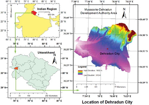
Dehradun is the capital of Uttarakhand, one of the northern states of India. The city of Dehradun including its surrounding Mussoorie Dehradun Development Authority area has been selected for the study. The geographical extents for the study area are located between latitude 30° 13’ 36.17” N to 30° 25’ 20.63” N and longitude 77° 52’ 24.64” E to 78° 9’ 39.70"E (Figure 2). The area is being developed as an alternative center called as counter magnet to accommodate migrated population due to population explosion in National Capital Region (NCR) of India (NCRPB 2008, NCRPB 2015). It is located in Doon Valley at the foothills of Himalayas. Climate of Dehradun is humid subtropical having hot summers and severe cold winters. Often, snowfall may be observed in the surrounding hilly region. Dehradun is nestled between River Ganges in the East and River Yamuna in the West; which are two major rivers in northern India. However, in this study area, only tributaries Song and Asan along with other smaller tributaries are present and carry discharge majorly during rainy season.

Figure 2. Location of the study area.

2.2. Data used

Landsat 8 OLI/TIRS data have been used in this study. One of the main reasons of using these data is the improved bandwidth of Bands 5 and 8. Band 5 is narrowed down to exclude water vapor absorption feature while width of Band 8 has been reduced to increase the contrast between vegetated areas and land without vegetation cover. Landsat 8 scene (Path 146 Row 39) of 10 December 2014 has been downloaded from http://earthexplorer.usgs.gov/. A subset image of this scene belonging to the study area has been extracted and OLI Bands 2–7 (Bands 2, 3, 4: Blue, Green, Red; Bands 5, 6, 7: NIR, SWIR1, SWIR2) and OLI Band 8 (PAN) have been used for present work. Other OLI/TIRS bands have been used as per requirement of computation of other indices which are required for a comparative assessment of NDAISI. Landsat 8 image used in this study has UTM map projection, WGS84 datum/ellipsoid in Zone 44N. Landsat 8 OLI data is acquired for nine spectral bands (Bands 1–7, 9) with a 30-m spatial resolution; however, PAN band (Band 8) has a resolution of 15 m. Landsat 8 level one terrain corrected product (L1T) available to users has been used and it is a radiometrically and geometrically corrected data. Other preprocessing carried out has been described in the subsequent paragraphs.

2.3. Data preprocessing

Cloud-free image acquired in good weather conditions has been used in this study, hence, atmospheric correction was not required (Deng and Wu 2012; Deng et al. 2015). DN values of OLI bands have been used for computation of MNDSI and as per requirement DN values were converted in to at-satellite reflectance for computation of other existing indices. A spatial enhancement of OLI multispectral bands (Band 2–7) has been carried out using high-resolution PAN band (Band 8). For spatial enhancement, a pan-sharpening technique, known as high-pass filter (HPF) resolution merge (Gangkofner, Pradhan, and Holcomb 2008) has been used.

In the present study area, river sediments were present in abundance in river beds, having similar pattern of spectral characteristics with impervious surfaces. Also, in greenness component as well as in average of brightness and wetness components of TC, separability between impervious surface and river sediments has been found least for TC image. Zhou et al. (2014) masked out river for computation of built-up and bare land index as river sediments were having similar spectral characteristics with bare land. Deng and Wu (2012) have suggested that prior to computation of BCI; masking of water bodies may be carried out. Further, it has been reported that shadows also have similar characteristics as impervious surfaces, in wetness component of TC (Deng and Wu 2012). Therefore, shadows, water, and river sediments were masked out from the image while computing BCI in this study. For identification of shadows, water and river sediments, an unsupervised classification using ISODATA algorithm was carried out.

2.4. Method

The method adopted for this study is shown by a flowchart (Figure 3). OLI Bands 2–7 have a spatial resolution of 30 m, while the spatial resolution of PAN Band 8 is 15 m. In order to obtain same spatial resolution, pan-sharpening was carried out using HPF resolution merge technique (Gangkofner, Pradhan, and Holcomb 2008). HPF merge algorithm involved five major steps viz. computation of the ratio (R) of cell size of multispectral image (Bands 2–7) to high resolution PAN band, creation of HPF image from PAN band using high pass kernel (HPK) based on R, re-sampling of low resolution image (Bands 2–7) to the pixel size of high-resolution PAN image, weighting of HPF image and addition to the multispectral image, and rescaling of output using linear stretch. For further details of these steps, Bhatti and Tripathi (2014) may be referred.

Figure 3. Flow chart of method.

For extraction and mapping of AIS, NDAISI was proposed. Computation of NDAISI required MNDSI, BCI, and RAISI (Figure 3). In the following subsections, methods of computing these indices and computation of NDAISI have been described. Also, methods of extraction and mapping of AIS, assessment of accuracy of results and their comparative assessment have been described.

2.4.1. Computation of MNDSI

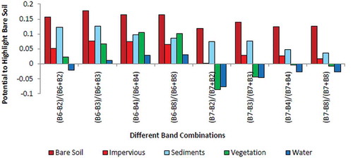
Areas of different classes of features, such as, impervious surfaces, bare soil, river sediment, vegetation, and water were demarcated on image by visual interpretation of the false-color composite using Bands 5, 4, and 3, respectively, in red, green, and blue channels. Signatures of these training samples were collected and a study on behavior of mean DN values has been carried out for Bands 2–8 (Figure 4) for computation of MNDSI to highlight bare soil. It is observed from Figure 4 that Bands 5, 6, and 7 exhibit higher mean values for bare soil while, Bands 2, 3, 4, and 8 have lower mean values. Further, vegetation also has a higher mean value in Band 5, so this band may be excluded in subsequent analysis for exploring two bands which may be used to compute MNDSI. Based on this, an exercise was carried out to identify the suitable band combination that highlights bare soil (Figure 5). It was observed that the componendo–dividendo relationship (normalized difference transformation) between Bands 7 (SWIR2) and Band 8 (PAN) highlights bare soil and separates it from river sediments and impervious surfaces effectively. Here, bare soil has significantly higher value when compared to other features, specifically values of impervious surfaces and sediments are close to zero, while vegetation and water have negative values. Bandwidth of PAN band of Landsat 8 OLI has been reduced in comparison to PAN band of Landsat 7 ETM+. OLI PAN band (0.50–0.68 μm) has wavelength range in visible region, while ETM+PAN band (0.52–0.90 μm) has wavelength ranging from visible to NIR. Perhaps, due to this reason OLI PAN band has helped to discriminate bare soil.

Figure 4. Average DN values of various feature classes in Bands 2–8 of Landsat 8 data.

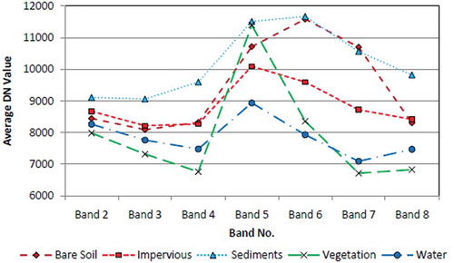
Figure 5. Higher potential of Bands 7 and 8 to highlight bare soil in comparison to other band combinations.

Based on above discussion, a Modified Normalized Difference Soil Index (MNDSI) was computed (Equation. 1) for Landsat 8 and subsequently used for improving capabilities of BCI to highlight AIS.

(1)

2.4.2. Computation of BCI

For computation of BCI, greenness and average of brightness and wetness components of TC were used (Deng and Wu 2012). TC transformation was carried out using Landsat 8 coefficients (Baig et al. 2014) for Bands 2–7 and BCI was computed as follows:

(2)

where H, L, and V are normalized brightness, wetness, and greenness components of TC. Most of spectral indices are designed to highlight one land cover while BCI addresses the confusion between impervious surfaces and bare soils. Values of BCI range from −1 to +1. However, BCI has moderate separability between impervious surfaces and bare soil and it may be further explored on this aspect (Deng and Wu 2012).

2.4.3. Computation of NDAISI

Improvement in the ability of BCI to highlight AIS has been carried out in two stages, to obtain enhanced discrimination between AIS and bare soil. In first stage, an intermediate enhancement of BCI was carried out which yielded a Ratio Anthropogenic Impervious Surface Index (RAISI). RAISI having an enhanced ability to discriminate between AIS and bare soil was computed as follows:

(3)

MNDSI_norm is normalized value of MNDSI ranging from 0 to 1. Now, to further enhance the ability to discriminate between AIS and bare soil in the second stage, new proposed index named as Normalized Difference Anthropogenic Impervious Surface Index (NDAISI) was computed as follows:

(4)

2.4.4. Extraction of AIS

Higher values of NDAISI indicate presence of AIS. A thresholding technique known as Double window Flexible Pace Search (DFPS) was used for extracting and mapping AIS by obtaining an optimum threshold value. DFPS was presented by Chen et al. (2003) for detecting optimum threshold value between change and no-change pixels for change detection of land use/land cover. He et al. (2010) developed and applied DFPS for determining optimal threshold value for extraction of built-up areas. Further, DFPS has been applied by Bhatti and Tripathi (2014) for extraction of built-up areas.

Initially, AIS training sample areas were selected by interpreting NDAISI image visually, in such a way that these include only AIS regions encircled by non-AIS pixels. For this, pure regions of AIS were identified and external boundaries were smoothly digitized in round shapes known as inner windows. Subsequently, outside boundaries to inner windows were created through buffering in ArcGIS 10.1 so that these were 1 or 2 pixels apart and contained non-AIS regions. These outer regions are known as outer windows, thus, double window areas of interest were created for collecting training samples. Thereafter, the process of finding an optimum threshold value was initiated using DFPS.

Range from minimum-to-maximum value of histogram, of an area of interest image defined for all training patches of inner windows, is known as search range, while search pace is an incremental value which divides search range in various segments to obtain various potential thresholds. The search range and pace were found on the basis of analysis of histogram of all training patches of pure regions of AIS for NDAISI. The first search pace i.e. increment (P₁) was computed as follows (He et al. 2010),

(5)

where, m is a positive integer, a and b are minimum and maximum values of search range, respectively. The number of potential thresholds in a search process was determined by m and its value was set manually. The value of m does not affect search efficiency and final results. A large value of m increases number of potential thresholds in a search, while number of searches is decreased. In a search process, potential thresholds to detect AIS pixels from training samples were computed as b-P₁, b-2P₁… within the range of b to a.

Further, performance of each threshold value during a search process was judged by its success rate (L_k) of AIS extraction.

(6)

where, A_k1 is number of AIS pixels detected inside all training patches (in the inner windows), A_k2 is number of AIS pixels detected incorrectly in the outside boundary of all training patches (in the outside windows), and A is total number of AIS pixels within all training patches (in the inner windows).

Finally, the iterative process of search when the difference of maximum and minimum success rate in a search process was found less than the error constant chosen as follows:

(7)

where, L_max and L_min are the maximum and minimum values of success rate in one search process and δ is an acceptable error constant. If the exit condition was not satisfied, a new search process was initiated. The new search process was set for the range from (k_{max –} P₁) to (k_max + P₁), where k_max is the potential threshold value corresponding to L_max in the search process. The new smaller search pace was set based on new search range using Equation (5). When the change of search pace has little influence on the result of AIS extraction, the threshold value corresponding to L_max was considered to be an optimal threshold value to extract AIS areas from NDAISI.

2.4.5. Assessment of accuracy

For assessment of accuracy, spatially enhanced Landsat 8 image, having resolution of 15 m was linked and synchronized with Google Earth using ERDAS Imagine 2014 software. Thus, high-resolution WorldView 2 images acquired on 23 February 2015 and made available by DigitalGlobe have been used as reference for assessment of accuracy. There is a lag of approximately two and half months in time of acquisition of Landsat 8 image used for study and WorldView 2 reference images, which may be acceptable.

Accuracy of extracted binary image was assessed by creating 250 stratified random points for AIS and non-AIS classes. The class value to these points was assigned on the basis of clear majority in a window of 3 pixels × 3 pixels in the binary image. All the points were checked with reference image and a reference class value was assigned for each binary image class value using accuracy assessment tool of ERDAS Imagine 2014. Thereafter, reports for accuracy totals and kappa statistics were generated. Assessment of accuracy was carried out for the results obtained from new NDAISI and existing approaches viz. BU_c and BAEM_OLI.

2.4.6. Comparative assessment

Comparative assessment was based on Spectral Discrimination Index (SDI) values (Pereira 1999), correlation analysis, visual comparison of results with available LULC map, and accuracy achieved. AIS maps were extracted using new NDAISI approach and existing BU_c and BAEM_OLI approaches. Water, shadow, and rivers were masked out from these maps from existing approaches for comparing results obtained from NDAISI. The comparative assessment of results has been carried out visually with available land use/land cover (LULC) map of study area. LULC map for the year 2011–2012 was obtained from Indian Geo-Platform Bhuvan, National Remote Sensing Centre (NRSC), Indian Space Research Organization (ISRO), Department of Space, India (http://bhuvan.nrsc.gov.in/gis/thematic/index.php). Source for preparation of this map at a scale of 1:50000, was terrain corrected Resourcesat-2 data from LISS III sensor having 23.5 m of spatial resolution. Overall accuracy of various classes of LULC map varies from 79% to 97%. Lower accuracy was achieved for class like agro-horticulture and highest was achieved for class like water bodies. For visual comparison, results of AIS were referred with the combination of two classes viz. built-up rural and built-up urban of LULC map.

3. Results and discussion

Initially, required indices MNDSI, BCI, and RAISI were computed and proposed NDAISI was created. Thereafter, extraction and mapping of AIS was carried out from new NDAISI as well as from existing BU_c and BAEM_OLI approaches. Accuracy of AIS maps was assessed and a comparative study of results obtained, from proposed and two existing approaches was carried out. The results are presented in the subsequent sections in sequential manner.

3.1. Computation of MNDSI

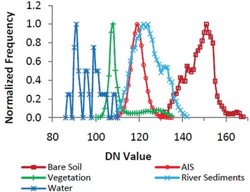
MNDSI was computed using Equation (1) and its values are ranging from −0.44 to 0.53 (Figure 6(a)). Figure 6(b) shows the histograms of various classes for unsigned 8 bit MNDSI image. It is observed that the histogram of bare soil is well separated from other classes. Mean of histograms for water, vegetation, and AIS are distinguished from mean of bare soil. The mean of histogram for river sediments is also distinguished from mean of bare soil; however, some overlapping may be seen by lower limbs. Further, in order to judge separability of other classes from bare soil, analysis of SDI has been carried out.

Figure 6a. Image of Modified Normalized Difference Soil Index.

Figure 6b. Histograms of the different classes for Modified Normalized Difference Soil Index.

Table 2 shows SDI of bare soil with other classes. It is found that SDI values of bare soil with impervious surface, vegetation, and water are greater than 1.96 and p-values are less than 0.05. This shows that mean value of impervious surfaces, vegetation, and water are statistically different from bare soil and there is no overlapping of histogram at 95% confidence level. However, SDI value of 1.79 for bare soil and river sediments is greater than 1.64 and p-value of 0.073 is less than 0.1. This shows that mean values of bare soil and river sediments are statistically different and that there is no overlapping of histograms at 90% confidence level.

Table 2. p-value and Spectral Discrimination Index of different classes with bare soil in Modified Normalized Difference Soil Index.

Class	Mean	Std. Dev	SDI with bare soil	p-Value
Bare soil	147.56	6.61	-	-
AIS	119.37	3.41	2.81*	0.004
River sediments	124.03	6.55	1.79**	0.073
Vegetation	112.11	8.22	2.39*	0.016
Water	96.50	5.99	4.05*	<0.001

*Mean values of two classes are statistically different at 95% confidence interval

**Mean values of two classes are statistically different at 90% confidence interval

3.2. Computation of NDAISI

For computation of NDAISI, BCI was generated using Equation (2). First-stage enhancement of BCI resulted in an intermediate ratio index (RAISI) using Equation (3). Subsequently, in second stage of enhancement, RAISI leads to NDAISI, which was computed using Equation (4). Computed NDAISI image is shown in Figure 7(a) having values from −1.0 to +1. Figure 7(b) shows the histograms for impervious surfaces and other classes for unsigned 8-bit NDAISI image. Histogram of impervious surface is well separated from other classes with virtually no overlap. However, an analysis of SDI has also been carried out.

Figure 7a. Image of Normalized Difference Anthropogenic Impervious Surface Index.

Figure 7b. Histograms of the different classes for Normalized Difference Anthropogenic Impervious Surface Index.

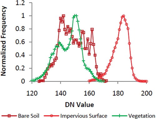
SDI values for bare soil and vegetation with respect to impervious surfaces are greater than 1.96 and p-values are less than 0.05 (Table 3). Therefore, mean values of bare soil and vegetation are statistically different from impervious surfaces and there is no overlap between histogram of other classes with impervious surfaces at 95% confidence level.

Table 3. p-value and Spectral Discrimination Index of different classes with Anthropogenic Impervious Surface in Normalized Difference Anthropogenic Impervious Surface Index.

Class	Mean	Std. Dev.	SDI with AIS	p-Value
AIS	181.67	5.54	-	-
Bare Soil	148.77	9.18	2.24*	0.025
Vegetation	144.68	10.70	2.28*	0.023

*Mean values of two classes are statistically different at 95% confidence interval

3.3. Extracting and mapping AIS

For extracting AIS, NDAISI image was normalized and converted into unsigned 8-bit integer such that the pixel values are ranging between 0 and 255. Histogram of NDAISI was analyzed for inner and outer window patches of training samples. Maximum and minimum values in all the inner window patches of AIS pixels were found to be 200 and 111, respectively. An optimum threshold value is expected to lie in the range from a = 111 to b = 200. Initially, the value of m was set to 9 and value of P₁ has been found approximately equal to 10 from Equation (5). Thereafter, an iterative search process was adopted and an optimum threshold value of 165 was obtained for NDAISI (Table 4). A similar exercise was carried out for BU_c and BAEM_OLI yielding the optimum threshold values 141 and 140, respectively.

Table 4. Search process for optimum threshold value using Double window Flexible Pace Search.

Range: 200–110 Pace 10		Range: 170–149 Pace 3		Range: 167–161 Pace 1
Threshold	Success rate	Threshold	Success rate	Threshold	Success rate
200	0.00%	170	66.84%	167	70.76%
190	1.05%	167	70.76%	166	71.00%
180	25.34%	164	70.95%	165	71.14%
170	66.84%	161	69.64%	164	70.95%
160	69.12%	158	67.58%	163	70.65%
150	61.72%	155	65.30%	162	70.12%
140	57.83%	152	63.01%	161	69.64%
130	56.16%	149	61.15%
120	54.39%
110	53.75%

In the present study, DFPS technique was used for an optimum threshold value. However, other available techniques may also be explored and their behavior may be studied. The NDAISI image was converted into binary image on the basis of optimum threshold obtained from DFPS. The binary image shows built-up areas by 1 and non-built-up areas by 0. The result of extracted map of AIS from NDAISI in the form of a binary image is shown in Figure 10(e). Similarly, AIS maps extracted from BU_c and BAEM_OLI are shown in Figure 10(c) and 10(d).

3.4. Assessment of accuracy

Assessment of accuracy was carried out and accuracy reports were obtained for AIS maps obtained for BU_c, BAEM_OLI, and NDAISI. From error matrix of AIS map from NDAISI, the small errors of omission (3.94%) and commission (4.69%) have been found for extracted AIS map. Results of accuracy totals are shown in Table 5 for AIS map from NDAISI. An overall accuracy of 95.60% is achieved and the overall kappa value of 0.912 has been found using NDAISI to extract impervious areas (Table 5). Results of assessment of accuracy for AIS maps from BU_c and BAEM_OLI have been discussed and compared with accuracy results of AIS map from NDAISI in the next section.

Table 5. Accuracy totals for Anthropogenic Impervious Surface map from Normalized Difference Anthropogenic Impervious Surface Index.

Class name	Reference totals	Classified totals	Number correct	Producers’ accuracy	Users’ accuracy
Non AIS	123	122	117
AIS	127	128	122	96.06%	95.31%
Totals	250	250	239
Overall accuracy 95.60%			Overall kappa 0.912

3.5. Comparative assessment of results

3.5.1. Comparison of SDI

SDI values of various classes were compared for NDVI, BU_c (improved NDBI), BCI, BAEM_OLI and proposed NDAISI. Figure 8 shows SDI values for different combination of feature classes amongst AIS, bare soil, and vegetation. It is found that NDAISI shows significantly high SDI values for AIS with both of bare soil and vegetation. The NDAISI has enhanced SDI value of AIS with bare soil when compared with NDVI, BUc, BCI, and BAEM_OLI. As the value of SDI is the difference of mean of two classes which is normalized by sum of standard deviations, thus a higher value of SDI indicates larger standardized difference in mean values. It is observed from Table 3 that for NDAISI, bare soil and vegetation have higher values of SDI when computed with respect to AIS. However, for other indices, SDI values of bare soil and AIS have been found less than 1 (Figure 8), which indicates a poor separability and lesser standardized difference in mean values between bare soil and AIS.

Figure 8. Spectral Discrimination Index of Anthropogenic Impervious Surface with other classes for different indices.

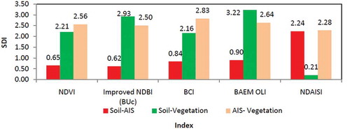
For AIS-Soil and AIS-Vegetation discrimination, SDI values are greater than 1.96 for NDAISI; thus, NDAISI is able to discriminate AIS from soil and vegetation at 95% confidence level. However, SDI value in NDAISI for AIS-Vegetation was found excellent but it has been slightly lowered in comparison to other evaluated indices. Further, SDI for Soil-Vegetation was found least in NDAISI in comparison to other evaluated indices, which does not impact discrimination of AIS from other features. Therefore, NDAISI discriminates AIS from bare soil effectively with little cost of lowered but excellent and significantly high SDI for AIS-Vegetation.

3.5.2. Correlation of NDAISI with other indices

Correlation of NDAISI with other indices such as, BCI, NDVI, BU_c, and BAEM_OLI has been carried out to observe its behavior in comparison to other indices. Table 6 shows correlation matrix of NDAISI and other indices. NDAISI has positive correlation with BCI, BU_c, and BAEM_OLI, while it is negatively correlated with NDVI. Positive correlation coefficient of NDAISI with BU_c is least, while it is highest with BCI. There is slightly higher correlation of NDAISI with BAEM_OLI when compared with BU_c. The indices BCI, BU_c, and BAEM_OLI have higher values for AIS with certain degree of confusion with bare soil, while NDVI has higher value for vegetation. Thus, BCI, BU_c, and BAEM_OLI highlight AIS and NDVI highlights vegetation. A positive or negative correlation of NDAISI with existing indices shows the agreement or disagreement with an index. Therefore, it may be concluded that NDAISI is able to highlight AIS as it has a positive correlation with BCI, BU_c, and BAEM_OLI and a negative correlation with NDVI.

Table 6. Correlation matrix of Normalized Difference Anthropogenic Impervious Surface Index and other indices.

	NDAISI	BCI	NDVI	BUc	BAEMOLI
NDAISI	1.000	0.857	−0.798	0.611	0.623

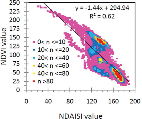
Figure 9(a) shows scatter plot of NDAISI and BCI. The scatter plot shows frequencies by different colors and clusters of high frequencies represent various classes of features. Scatter plot is based on samples taken for AIS, bare soil, and vegetation in proportion to area covered by them; the frequencies also vary for different LULC. Linear relationship between NDAISI and BCI shows a positive slope (m) and strong correlation (m = 1.18, R² = 0.73) (Figure 9(a)). Similarly, NDVI has a negative slope and strong correlation (m = −1.44, R² = 0.62) (Figure 9(b)). BUc and BAEM_OLI have positive slope (m = 1.09 and 1.11, respectively) and weak correlation (R² = 0.36 for both). However, correlations of NDAISI, with all other evaluated indices, may be positive or negative, have been found significant at 95% confidence level (p-value <0.00001). Figure 9(a) and Figure 9(b), respectively, show the scatter plots of NDAISI with one of the indices having positive (BCI) and negative (NDVI) correlation each.

Figure 9a. Scatter-plot of Normalized Difference Anthropogenic Impervious Surface Index and Biophysical Composition Index showing positive correlation.

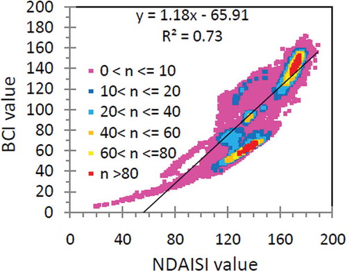
Figure 9b. Scatter-plot of Normalized Difference Anthropogenic Impervious Surface Index and Normalized Difference Vegetation Index showing negative correlation.

3.5.3. Comparison of results

Results of AIS maps obtained from BU_c and BAEM_OLI approaches have been compared with the results of AIS map from NDAISI. Subsequently, results from all three approaches have been compared with LULC map of 2011–2012 obtained from NRSC (Figure 10). Images of actual indices BU_c and BAEM_OLI are shown in Figure 10(a) and 10(b), respectively, while image of actual index NDAISI is shown in Figure 7(a). The areas of AIS extracted from three approaches are shown in bright, while the background is shown in dark (Figure 10(c)–(e)). Figure 10(c)–(e) show results obtained from BU_c, BAEM_OLI and proposed NDAISI approaches, respectively, while LULC map is shown in Figure 10(f). The study area consists of variety of classes of features, which include forest (evergreen, deciduous, plantation, and scrub), agricultural (crop, plantation, and fallow land), built–up (urban and rural), barren and water (Figure 10(f)). Area of present study has good degree of heterogeneity of features.

Figure 10. Results obtained from (a) image of BU_c index (b) Image of BAEM_OLI index (c) AIS map from Improved NDBI (BU_c), (d) AIS map from BAEM_OLI, (e) AIS map from NDAISI, and (f) LULC map.

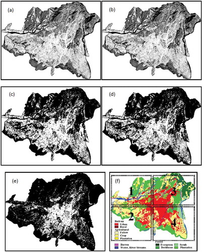
For comparing results, study area was divided in four zones viz. Zone 1, Zone 2, Zone 3, and Zone 4 as shown in Figure 10(f) by dotted rectangles. Larger view of results obtained from three different approaches in zones 2 is shown in Figure 11 and it was compared visually. Further, some of the areas were marked out by different shapes for closer look. In general, BU_c (Figure 11(a)) and BAEM_OLI (Figure 11(b)) show the presence of larger areas of AIS within marked shapes when compared with respective LULC map of zone 2 (Figure 11(d)). An overestimation of anthropogenic impervious surface has been observed by BU_c and BAEM_OLI approaches. However, results obtained from NDAISI show presence of lesser areas of anthropogenic impervious surfaces (Figure 11(c)) and are found in close agreement with respective LULC map of zone 2 (Figure 11(d)). The comparison of actual images of indices BU_c, BAEM_OLI (Figure 10(a) and 10(b)), and NDAISI (Figure 7(a)) also show overestimation of AIS from by BU_c and BAEM_OLI. A similar observation has been found in all four zones.

Figure 11. Comparison of zone 2, (a) AIS map from improved NDBI (BU_c), (b) AIS map from BAEM_OLI, (c) AIS map from NDAISI, and (d) LULC map.

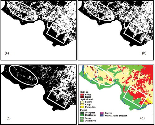
The heterogeneity of features present in study area and presence of bare soil in abundance may have influence on the performance of BU_c and BAEM_OLI. The overestimation of AIS by BU_c and BAEM_OLI approaches may be due to lesser separability and confusion between bare soil and AIS. From comparative study in four zones, it is observed that first two approaches i.e. improved NDBI (BU_c) and BAEM_OLI are not able to separate bare soil and impervious surfaces effectively and confusion between these has been found. However, NDAISI approach has resulted in significantly improved results in all four zones.

3.5.4. Comparison of accuracy achieved

The accuracy achieved for AIS area mapping using all three approaches is shown in Table 7. Overall accuracies achieved are 72%, 72.8%, and 95.6% for BU_c, BAEM_OLI, and NDAISI approaches, respectively. Commission error has been greatly reduced at a little cost of omission error in NDAISI approach. The kappa coefficient has significantly higher value for NDAISI in comparison to evaluated existing approaches. The new AIS extraction and mapping approach has provided best result with significant improvement over improved NDBI (BU_c) and BAEM_OLI approaches.

Table 7. Comparison of accuracy of results obtained from different approaches.

Approach	Overall accuracy (%)	Omission error (%)	Commission error (%)	Kappa coefficient
Improved NDBI (BUc)	72.00	0.98	40.59	0.474
BAEMOLI	72.80	2.86	38.92	0.484
NDAISI	95.60	3.94	4.69	0.912

From above discussion, it is evident that MNDSI and NDAISI have been useful for extracting and mapping of AIS. However, for improving overall discrimination of classes in general, some of the recent techniques are being used. These techniques are based on spectral texture, multisource classification, object-oriented analysis, knowledge-based classification, spectral mixture analysis, neural network, and decision tree classification. For improving discrimination of classes and accuracy of classification results, various indices have been used in combination of raw satellite data to form a composite image. For this purpose, usefulness of MNDSI and NDAISI may be explored.

4. Conclusions

AIS extraction approach, using proposed Normalized Difference Anthropogenic Impervious Surface Index (NDAISI), has shown very encouraging results. NDAISI was computed using Modified Normalized Difference Soil Index (MNDSI) and Ratio Anthropogenic Impervious Surface Index (RAISI). The RAISI was computed from Biophysical Composition Index (BCI) and MNDSI. NDAISI shows great improvement in spectral discrimination of AIS with bare soil when compared to BCI, BU_c, and BAEM_OLI. The AIS have been extracted using Double window Flexible Search (DFPS) thresholding technique from NDAISI and results have been compared with improved NDBI (BU_c) and BAEM_OLI approaches. It is found that there is a significant improvement in extracting AIS viz. a viz. other classes, such as, vegetation and bare soil, etc.

Acknowledgments

This study has been carried out under a doctoral program supported by the Ministry of Human Resource Development, India. The first author gratefully acknowledges the MHRD, India, for financial support. Authors acknowledge USGS and NRSC for data used in the study. Authors are thankful to the editor and anonymous reviewers for suggestive comments which have supported to improve the manuscript.

Disclosure statement

No potential conflict of interest was reported by the authors.

Additional information

Funding

The first author was supported by the Ministry of Human Resource Development, Government of India, for this work.

References

- Anderson, J. R. 1976. A Land Use and Land Cover Classification System for Use with Remote Sensor Data. Vol. 964. Washington, DC: US Government Printing Office.
- As-Syakur, A. R., I. W. S. Adnyana, I. W. Arthana, and I. W. Nuarsa. 2012. “Enhanced Built-Up and Bareness Index (EBBI) for Mapping Built-Up and Bare Land in an Urban Area.” Remote Sensing 4 (10): 2957–2970. doi:10.3390/rs4102957.
- Baig, Muhammad Hasan Ali.., L. Zhang, T. Shuai, and Q. Tong. 2014. “Derivation Of A Tasselled Cap Transformation Based On Landsat 8 At-satellite Reflectance.” Remote Sensing Letters 5 (5): 423–431. doi:10.1080/2150704X.2014.915434.
- Bauer, M. E., N. J. Heinert, J. K. Doyle, and F. Yuan. 2004. “Impervious Surface Mapping and Change Monitoring Using Landsat Remote Sensing.” In ASPRS annual conference proceedings, vol. 10. Bethesda, MD: American Society for Photogrammetry and Remote Sensing.
- Bhatti, S. S., and N. K. Tripathi. 2014. “Built-Up Area Extraction Using Landsat 8 OLI Imagery.” Giscience & Remote Sensing 51 (4): 445–467. doi:10.1080/15481603.2014.939539.
- Census of India. 2011. Metadata. Office of the Registrar General & Census Commissioner, India. http://www.censusindia.gov.in/2011census/HLO/Metadata_Census_2011.pdf
- Chen, J., P. Gong, C. He, R. Pu, and P. Shi. 2003. “Land-Use/Land-Cover Change Detection Using Improved Change-Vector Analysis.” Photogrammetric Engineering & Remote Sensing 69 (4): 369–379. doi:10.14358/PERS.69.4.369.
- Chen, Y., P. Shi, T. Fung, J. Wang, and X. Li. 2007. “Object‐Oriented Classification for Urban Land Cover Mapping with ASTER Imagery.” International Journal of Remote Sensing 28 (20): 4645–4651. doi:10.1080/01431160500444731.
- Deng, C., and C. Wu. 2012. “BCI: A Biophysical Composition Index for Remote Sensing of Urban Environments.” Remote Sensing of Environment 127: 247–259. doi:10.1016/j.rse.2012.09.009.
- Deng, Y., C. Wu, M. Li, and R. Chen. 2015. “RNDSI: A Ratio Normalized Difference Soil Index for Remote Sensing of Urban/Suburban Environments.” International Journal of Applied Earth Observation and Geoinformation 39: 40–48. doi:10.1016/j.jag.2015.02.010.
- DOE (Department of the Environment). 1975. National Land Use Classification. Londan: HMSO.
- Gangkofner, U. G., P. S. Pradhan, and D. W. Holcomb. 2008. “Optimizing the High-Pass Filter Addition Technique for Image Fusion.” Photogrammetric Engineering & Remote Sensing 74: 1107–1118. HPF Resolution Merge. In: ERDAS IMAGINE Help. Leica Geosystems Geospatial Imaging, LLC. doi:10.14358/PERS.74.9.1107.
- George, X., C. Mike, and C. McMahon. 2008. “Quantifying Multi-Temporal Urban Development Characteristics in Las Vegas from Landsat and ASTER Data.” Photogrammetric Engineering & Remote Sensing 74 (4): 473–481. doi:10.14358/PERS.74.4.473.
- Hao, P., Z. Niu, Y. Zhan, Y. Wu, L. Wang, and Y. Liu. 2016. “Spatiotemporal Changes of Urban Impervious Surface Area and Land Surface Temperature in Beijing from 1990 to 2014.” Giscience & Remote Sensing 53: 63–84. doi:10.1080/15481603.2015.1095471.
- Harrison, A. R. 2006. National Land Use Database: Land Use and Land Cover Classification (Version 4.4). Office of the Deputy Prime Minister, Queen’s Printer and Controller of Her Majesty’s Stationery Office, London, UK.
- He, C., P. Shi, D. Xie, and Y. Zhao. 2010. “Improving the Normalized Difference Built-Up Index to Map Urban Built-Up Areas Using a Semiautomatic Segmentation Approach.” Remote Sensing Letters 1 (4): 213–221. doi:10.1080/01431161.2010.481681.
- Kawamura, M., S. Jayamana, and Y. Tsujiko. 1996. “Relation between Social and Environmental Conditions in Colombo Sri Lanka and the Urban Index Estimated by Satellite Remote Sensing Data.” International Archives of Photogrammetry and Remote Sensing 31: 321–326.
- Li, W., and C. Wu. 2016. “A Geostatistical Temporal Mixture Analysis Approach to Address Endmember Variability for Estimating Regional Impervious Surface Distributions.” Giscience & Remote Sensing 53: 102–121. doi:10.1080/15481603.2015.1118975.
- Liu, J., H. Tian, M. Liu, D. Zhuang, J. M. Melillo, and Z. Zhang. 2005. “China’s Changing Landscape during the 1990s: Large‐Scale Land Transformations Estimated with Satellite Data.” Geophysical Research Letters 32 (2). doi:10.1029/2004GL021649.
- Lu, D., E. Moran, and S. Hetrick. 2011. “Detection of Impervious Surface Change with Multitemporal Landsat Images in an Urban–Rural Frontier.” ISPRS Journal of Photogrammetry and Remote Sensing 66 (3): 298–306. doi:10.1016/j.isprsjprs.2010.10.010.
- Mas, J. F. 2004. “Mapping Land Use/Cover in a Tropical Coastal Area Using Satellite Sensor Data, GIS and Artificial Neural Networks.” Estuarine, Coastal and Shelf Science 59 (2): 219–230. doi:10.1016/j.ecss.2003.08.011.
- NCRPB (National Capital Region Planning Board). 2008. A Study on Counter-Magnet Areas to Delhi and National Capital Region. Ministry of Urban Development, Government of India, New Delhi.
- NCRPB (National Capital Region Planning Board). 2015. Annual Report 2014-15. Ministry of Urban Development, Government of India, New Delhi.
- Parece, T. E., and J. B. Campbell. 2013. “Comparing Urban Impervious Surface Identification Using Landsat and High Resolution Aerial Photography.” Remote Sensing 5 (10): 4942–4960. doi:10.3390/rs5104942.
- Pereira, J. M. 1999. “A Comparative Evaluation of NOAA/AVHRR Vegetation Indexes for Burned Surface Detection and Mapping.” IEEE Transactions on Geoscience and Remote Sensing 37 (1): 217–226. doi:10.1109/36.739156.
- Slonecker, E. T., D. B. Jennings, and D. Garofalo. 2001. “Remote Sensing of Impervious Surfaces: A Review.” Remote Sensing Reviews 20 (3): 227–255. doi:10.1080/02757250109532436.
- Squires, G. 2012. Urban and Environmental Economics: An Introduction. Abingdon: Routledge.
- Stathakis, D., K. Perakis, and I. Savin. 2012. “Efficient Segmentation of Urban Areas by the VIBI.” International Journal of Remote Sensing 33 (20): 6361–6377. doi:10.1080/01431161.2012.687842.
- Thompson, M. 1996. “A Standard Land-Cover Classification Scheme for Remote-Sensing Applications in South Africa.” South African Journal of Science 92 (1): 34–42.
- Torbick, N., and M. Corbiere. 2015. “Mapping Urban Sprawl and Impervious Surfaces in the Northeast United States for the past Four Decades.” Giscience & Remote Sensing 52 (6): 746–764. doi:10.1080/15481603.2015.1076561.
- Weng, Q. 2012. “Remote Sensing of Impervious Surfaces in the Urban Areas: Requirements, Methods, and Trends.” Remote Sensing of Environment 117: 34–49. doi:10.1016/j.rse.2011.02.030.
- Xiao, J., Y. Shen, J. Ge, R. Tateishi, C. Tang, Y. Liang, and Z. Huang. 2006. “Evaluating Urban Expansion and Land Use Change in Shijiazhuang, China, by Using GIS and Remote Sensing.” Landscape and Urban Planning 75 (1): 69–80. doi:10.1016/j.landurbplan.2004.12.005.
- Xu, H. 2006. “Modification Of Normalised Difference Water Index (Ndwi) To Enhance Open Water Features In Remotely Sensed Imagery.” International Journal Of Remote Sensing 27 (14): 3025-3033. doi:10.1080/01431160600589179.
- Xu, H. 2007. “Extraction of Urban Built-Up Land Features from Landsat Imagery Using a Thematic Oriented Index Combination Technique.” Photogrammetric Engineering & Remote Sensing 73 (12): 1381–1391. doi:10.14358/PERS.73.12.1381.
- Xu, H. 2008. “A New Index for Delineating Built-Up Land Features in Satellite Imagery.” International Journal of Remote Sensing 29 (14): 4269–4276. doi:10.1080/01431160802039957.
- Xu, H. 2010. “Analysis of Impervious Surface and Its Impact on Urban Heat Environment Using the Normalized Difference Impervious Surface Index (NDISI).” Photogrammetric Engineering & Remote Sensing 76 (5): 557–565. doi:10.14358/PERS.76.5.557.
- Yuan, F., C. Wu, and M. E. Bauer. 2008. “Comparison of Spectral Analysis Techniques for Impervious Surface Estimation Using Landsat Imagery.” Photogrammetric Engineering & Remote Sensing 74 (8): 1045–1055. doi:10.14358/PERS.74.8.1045.
- Zha, Y., J. Gao, and S. Ni. 2003. “Use of Normalized Difference Built-Up Index in Automatically Mapping Urban Areas from TM Imagery.” International Journal of Remote Sensing 24 (3): 583–594. doi:10.1080/01431160304987.
- Zhang, J., L. Zhengjun, and S. Xiaoxia. 2009. “Changing Landscape in the Three Gorges Reservoir Area of Yangtze River from 1977 to 2005: Land Use/Land Cover, Vegetation Cover Changes Estimated Using Multi-Source Satellite Data.” International Journal of Applied Earth Observation and Geoinformation 11 (6): 403–412. doi:10.1016/j.jag.2009.07.004.
- Zhou, Y., G. Yang, S. Wang, L. Wang, F. Wang, and X. Liu. 2014. “A New Index for Mapping Built-Up and Bare Land Areas from Landsat-8 OLI Data.” Remote Sensing Letters 5 (10): 862–871. doi:10.1080/2150704X.2014.973996.
- Zhu, G., and D. G. Blumberg. 2002. “Classification Using ASTER Data and SVM Algorithms;: The Case Study of Beer Sheva, Israel.” Remote Sensing of Environment 80 (2): 233–240. doi:10.1016/S0034-4257(01)00305-4.