Time-series cloud noise mapping and reduction algorithm for improved vegetation and drought monitoring

Abstract

Moderate Resolution Imaging Spectro-radiometer (MODIS) time-series Normalized Differential Vegetation Index (NDVI) products are regularly used for vegetation monitoring missions and climate change analysis. However, satellite observation is affected by the atmospheric condition, cloud state and shadows introducing noise in the data. MODIS state flag helps in understanding pixel quality but overestimates the noise and hence its usability requires further scrutiny. This study has analyzed MODIS MOD09A1 annual data set over Sri Lanka. The study presents a simple and effective noise mapping method which integrates four state flag parameters (i.e. cloud state, cloud shadow, cirrus detected, and internal cloud algorithm flag) to estimate Cloud Possibility Index (CPI). Usability of CPI is analyzed along with NDVI for noise elimination. Then the gaps generated due to noise elimination are reconstructed and performance of the reconstruction model is assessed over simulated data with five different levels of random gaps (10–50%) and four different statistical measures (i.e. Root mean square error, mean absolute error, mean bias error, and mean absolute percentage error). The sample-based analysis over homogeneous and heterogeneous pixels have revealed that CPI-based noise elimination has increased the detection accuracy of number of growing cycle from 45–60% to 85–95% in vegetated regions. The study cautions that usage of time-series NDVI data without proper cloud correction mechanism would result in wrong estimation about spatial distribution and intensity of drought, and in our study 50% of area is wrongly reported to be under drought though there was no major drought in 2014.

Keywords:

• MODIS NDVI
• time-series noise reduction
• cloud possibility index
• growth cycle
• drought assessment

1. Introduction

In the past two decades, usage of time-series satellite data has increased manifold due to coherent and long-term archival data being freely available at a high temporal resolution across the globe (Erasmi, Bothe, and Petta 2006; Hamandawana, Eckardt, and Chanda 2005). The time-series data is used for studying global to local-level changes in the terrestrial vegetation (Brown et al. 2008; Jakubauskas, Legates, and Kastens 2002; Jeganathan, Dash, and Atkinson 2014; Reed 2006; Tadesse et al. 2010; Tian et al. 2015; Zhang et al. 2003). Among the many time-series data, NDVI product from Advanced Very High Resolution Radiometer (AVHRR) (Eastman et al. 2013; Heumann et al. 2007; Luo et al. 2013; Wang and Tenhunen 2004) and Moderate Resolution Imaging Spectro-radiometer (MODIS) (Beck et al. 2006; Luo et al. 2013; Zhang et al. 2003) have been utilized extensively to understand the vegetation dynamics (Jeganathan and Nishant 2014; Sakamoto et al. 2010; Zhang et al. 2003) in response to climatic fluctuation, drought impact (Ji and Peters 2003) as well as human activity. Recently, number of studies using time-series NDVI for regional drought monitoring has increased and they contributed in understanding spatiotemporal dynamics of drought events such as intensity, duration, and spatial coverage (Ghaleb, Mario, and Sandra 2015).

However, atmospheric condition, cloud and shadow, and bidirectional effect introduces noise and degrades the data quality (Atkinson et al. 2012; De Oliveira, Epiphanio, and Rennó 2014; Jia et al. 2011; Roy et al. 2002). The abnormality in NDVI values with irregular data gaps limits the accurate estimation of terrestrial dynamics (Michishita et al. 2014). Numerous studies have successfully experimented several noise reduction and smoothing techniques, including 4253H filter (Velleman 1980), Savitzky-Golay filter (Chen et al. 2004; Jönsson and Eklundh 2004; Savitzky and Golay 1964), Weighted least square regression approach (Swets et al. 1999), Asymmetric Gaussian (Jonsson and Eklundh 2002; Jönsson and Eklundh 2004), Whittaker smoother (Atzberger and Eilers 2011), Double logistic (Beck et al. 2006; Zhang et al. 2003), Best slope index Condition (Lovell and Graetz 2001; Viovy, Arino, and Belward 1992), Harmonic analysis (Bradley et al. 2007), Discrete Fourier transformation (Atkinson et al. 2012; Bradley et al. 2007; Brooks et al. 2012; Jeganathan, Dash, and Atkinson 2010; McCloy and Lucht 2004; Roerink, Menenti, and Verhoef 2000), Wavelet transformation (Chen et al. 2011; Lu et al. 2007; Sakamoto et al. 2010), Mean value iteration (Ma and Veroustraete 2006), Window regression-based approach (De Oliveira, Epiphanio, and Rennó 2014), and spatiotemporal interpolation (Cho and Suh 2013; De Oliveira and Epiphanio 2012; Poggio, Gimona, and Brown 2012; Weiss et al. 2014). However, only in few studies the MODIS quality flag is utilized prior to smoothing. MODIS provides composite-wise quality information at each pixel for 1-km and 250-m VI products, and two different quality information (i.e. quality assessment flag and state flag) for 500-m surface reflectance product. The state quality flag mainly contains cloud and associated noise information of a pixel. However, studies found that there is an inherent uncertainty in the quality flag and hence the pixel marked as low or high quality need to be considered with caution (De Oliveira, Epiphanio, and Rennó 2014; Grogan and Fensholt 2013; Hilker et al. 2012). More recently, De Oliveira, Epiphanio, and Rennó (2014) used a spatiotemporal window regression-based condition, where the noisy value identified using MODIS quality information is replaced by the neighboring pixel value having lowest temporal variance. However, using the spatial window-based model, estimation of the correct value is always difficult for the pixel having heterogeneous land cover in the neighborhood (especially due to coarser spatial resolution). In addition, cloud masking process generates data gaps in the time-series and hence gap filling is an important step in the reconstruction process. Kandasamy et al. (2013) studied 8 different gap filling techniques and found that local temporal window-based techniques performed better in eliminating gaps than the global techniques (which utilizes whole time-series) but they could not eliminate long gaps.

Therefore, the present study attempts to test the noise detection ability of MODIS quality flag and to develop simple, robust, and reproducible approaches to identify and eliminate the cloud-induced noise and gaps in time-series NDVI. The study is carried out over Sri Lanka which receives two rainy seasons: Yala (December to March) and Maha (May to September), and hence remote sensing data are highly affected by cloud cover. Therefore, removal of cloud noise from time-series RS data is a necessity for environmental applications.

2. Methodology

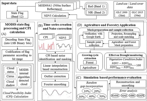
In this study, surface reflectance (RED and Near Infrared [NIR] bands) and state flag data (MOD09A1-V5) of on-board MODIS Terra sensor (500-m spatial resolution and 8-day temporal resolution) are used as main input data. Two horizontally successive tiles (h25v08 and h26v08) covering full Sri Lanka are downloaded for 14 years (2001 to 2014). All the experiments are carried out over one year (2014) data, and all the 14 years of data are used to derive long-term statistics for drought application. User needs to compute the NDVI using RED and NIR bands, and there is no maximum value composited NDVI product available at 500-m spatial resolution. Therefore, two additional flags for quality information (i.e. Quality Assessment [QA] flag and state flag) are provided to allow the user to explore on their own. In addition, Global Land Cover (GLC2000) (Bartholomé and Belward 2005) (1-km resolution) is used to identify various forest and agriculture classes, and Global Land Cover map (Chen et al. 2015) derived using 30-m Landsat data (GLC30) is used as a reference to identify homogeneous and heterogeneous sample pixels and to evaluate the results over forested and agriculture regions. Figure 1 provides the overall methodology followed in this study. The whole study is divided into four parts to achieve the objective. First, cloud information from the MODIS 500-m state flag is integrated to derive a cloud possibility index (CPI). Second, CPI and NDVI values are analyzed together for noise identification and elimination. Third, carrying out gap filling and performance evaluation of gap reduction method. Finally, evaluation of performance of the whole approach is carried out for two different applications: vegetation growth information extraction and drought assessment.

Figure 1. Overall methodology of the study. For full colour versions of the figures in this paper, please see the online version.

2.1. Cloud possibility index

MODIS Land (MODLAND) science team provides pixel-wise quality assurance data for each composite. The MOD09A1 Science Data Set contains 12 bands, including two quality-related data: (a) surface reflectance quality band; and (b) state flags (16 bit) band. The surface reflectance quality band (band 8) provides overall pixel reliability information and band-wise pixel reliability assessment parameter, whereas, the state flag (band 12) provides information about the nature of noise such as cloud, cloud shadow, aerosol quantity, cirrus, bidirectional reflectance distribution function etc. The qualitative noise parameter is represented by binary codification which is encoded into integer format. The user needs to decode it into a little endian binary format to obtain proper bit-wise information (Vermote, Kotchenova, and Ray 2015).

Therefore, appropriate bit combinations are used to extract multiple quality parameter, and each parameter is converted into a separate band. In this study, we have used four cloud related parameter i.e. Cloud State, Cloud Shadow, Cirrus detected, and MODIS cloud flag parameter. Each parameter contains further subcategories representing the degree of noise information. We have integrated these four parameters through a rating (Table 1)-based weighted sum process (i.e. parameters are rated first and then summed) and created a CPI to quantitatively assess noise intensity in a pixel. The details about bit information, parameters, rating and attribute details are provided in Table 1 for ready reference to the readers.

Table 1. Attribute class rating in MODIS 500-m state flag (16 bit).

*Bit no.	Band no.	*Parameter name	*Bit combination.	Cloud rating code	*Attribute class
0–1	Band 1	Cloud state	00	0	Clear
			11	1	Not set, assumed clear
			10	2	Mixed
			01	3	Cloudy
2	Band 2	Cloud shadow	0	0	No
			1	2	Yes
8–9	Band 3	Cirrus detected	00	0	None
			01	1	Small
			10	2	Average
			11	3	High
10	Band 4	Internal cloud algorithm flag	0	0	No cloud
			1	2	Cloud

*Source: Modis user guide (Vermote, Kotchenova, and Ray 2015)

2.2. Noise elimination and reconstruction

2.2.1. CPI- and NDVI-based noise detection

The bands 1 and 2 (MOD09A1) representing the surface reflectance information in RED and NIR wavelength regions are used to compute NDVI for all the composites, and an annual time-series stack of NDVI (46 composites) is created covering January to December months in 2014. Similarly, CPI is computed for all the 46 composites and an annual CPI time-series stack is created.

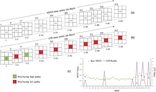
Figure 2 illustrates the conceptual relationship between the time-series NDVI value and CPI value (as an example case). The low-quality pixel (marked in red color in Figure 2a and 2b) in a composite is characterized by the higher CPI value. The higher CPI value and corresponding lower NDVI value depicts the inverse relationship between cloud-induced noise and NDVI value. In Figure 2b, the major noise (CPI ≥2) could be observed in 8 composites out of 46 composites (one-year time-series). The lower NDVI value in 40th and 44th composite (Figure 2c) having CPI = 8 reveals that magnitude of NDVI value is inversely dependent on the amount of noise. Hence, we can identify noisy NDVI values with the assistance of the CPI value (Eqn. 1).

(1)

Figure 2.  Graphical representation of time-series NDVI and CPI values extracted from MODIS 500 m data of 2014: (a) time-series NDVI, (b) time-series CPI, and (c) relationship between time-series NDVI and CPI values.

Where, is the CPI value of i_th composite and is the CPI threshold. However, due to uncertainty in the MODIS state flag this relationship between CPI and NDVI value is not always reliable (Letu et al. 2014). Therefore, to address this issue we have incorporated an additional NDVI-based condition (Equation 2) in addition to Equation (1) so as to identify and mask-out correct noisy NDVI value.

(2)

(3)

(4)

Where, CPI_i is the CPI value at i_th composite, CPI_β is the CPI threshold, NDVI_i is the NDVI value at i_th composite, is the annual mean NDVI, is the standard deviation of annual time-series NDVI, is the Threshold Controlling Factor (TCF) having value from −1 to +1 and N is the total number of NDVI composites. Five different values of TCF are tested in this study (Table 2). In this step, temporal neighbors are not considered.

Table 2. Six cloud noise detection conditions used in the study.

Threshold based condition	Value of TCF	Actual form of masking condition
TBC 1	-
TBC 2	1
TBC 3	0.5
TBC 4	0
TBC 5	−0.5
TBC 6	−1

2.2.2. Gap filling and reconstruction of time-series NDVI

The gap filling and reconstruction approach consist of three major steps, i.e. (1) filling the gaps generated by the noise elimination process, (2) removing the local fluctuation using temporal moving window-based filter, and (3) generating smooth time-series data.

A temporal moving window-based technique is used to fill the gaps. For each pixel, all the Vegetation Index (VI) values at time “” are checked for gaps, and a rate of change-based linear interpolation technique is used (Equations 5, 6, 7, and 8) to estimate the predicted NDVI value. The advantage of this approach is that lengthy gap can also be filled.

(5)

The “” represents the rate of change in VI value between neighborhood time range:

(6)

Where,

(7)

(8)

Where, is the current composite time (in composite number); is the timing of preceding non-noisy neighbor value; is the timing of succeeding non-noisy neighbor value; is the difference between non-noisy succeeding and preceding VI value; and is the time difference (in terms of number of composites) between succeeding and preceding non-noisy value location. Annual cyclicity is assumed to maintain the continuity while searching for preceding or succeeding neighbors (for example, if the preceding neighbor is not found till the first composite then the search will continue from the last composite cyclically and vice versa for succeeding neighbors). In this regard, the difference in location and value is calculated by considering the total number of the time gap in the loop. However, the quality of the new data fully depends on the number of noisy or non-noisy values and the length of the gap in a temporal profile (Justice et al. 2002).

The local fluctuation or statistical outlier in NDVI values cannot be detected by using MODIS state flag alone (Letu et al. 2014). Hence, after filling the gaps, a statistical envelop-based filter is used to check for any possible local fluctuation. The upper and lower threshold limits are derived using mean and standard deviation of the two temporal neighbors on both sides of the current position (Eqn. 9).

(9)

Where,

(10)

and

(11)

Where, and are the mean and standard deviation, respectively, of two previous and the two-successive neighborhood VI values, n is the window size (i.e. total number of neighbors), is the VI value of the i_th temporal band, is the VI value of current time, is the VI value at the previous immediate time and is the VI value at the next immediate time.

Finally, harmonic-series-based Discrete Fourier Transformation (DFT) has been used for smoothing time-series NDVI data to facilitate automatic information extraction. The merit of DFT-based smoothing over other competitive technique is widely evaluated in Atkinson et al. (2012) and utilized in Jeganathan, Dash, and Atkinson (2010) and Dash, Jeganathan, and Atkinson (2010) for vegetation growth monitoring. The DFT decomposes any complex time-series data into a series of simple waves of different frequency (i.e., harmonics), and inverse DFT using coefficients from lower order harmonics would result in smoothed annual data.

The Fourier Smoothing (FS) is based on the sum of sine and cosine functions that describes the periodic signal.

(12)

The equation consists of two parts: real or cosine part and imaginary or sine part.

The cosine part is:

(13)

The sine part is:

(14)

Where, is the VI value in the time-series, is the mean annual VI, is the harmonic component of Fourier transformation, is the time of and N is the length of the total time period (i.e. total number of composites). For a smooth reconstruction of annual time-series, consideration of the appropriate number of harmonics is very important. The first two harmonics can take into account about 50–90% of the variability in a time-series (Jakubauskas, Legates, and Kastens 2001). However, only two harmonics components do not reproduce reliable time-series. Therefore, four to six harmonics are usually recommended for correct identification of different land cover features, and to accurately identify various phenological metrics (e.g., the number of growing season, sowing and harvesting time, etc.) (Atkinson et al. 2012; Jeganathan, Dash, and Atkinson 2010).

2.3. Sensitivity test for the gap filling model

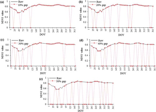
The sensitivity analysis of any reconstruction approach is important to evaluate performance of the model. However, the major problem is how to evaluate a reconstructed profile in the absence of error free data. Therefore, the sensitivity of the proposed gap filling model is evaluated based on Monte Carlo simulation as followed in Zhou et al. (2012). During simulation, we have introduced artificial gaps at random locations in a time-series NDVI. Five different percentages (10%, 20%, 30%, 40%, and 50%) of random data gaps equivalent to dropouts of 4, 9, 13, and 18 composites, respectively, are tested over 100 different NDVI profiles (one sample profile is provided in Figure 3). Finally, the simulated datasets are reconstructed using proposed gap filling model.

Figure 3.  Simulated annual NDVI profile having different percentages of random gaps: (a) 10%, (b) 20%, (c) 30%, (d) 40%, and (e) 50%

In order to quantitatively evaluate the performance, four different statistical measures i.e. root mean square Error (RMSE), mean absolute error (MAE), mean bias error (MBE), and mean absolute percentage error (MAPE) are used. RMSE is one of the traditional techniques used to describe the nature of the fit between predicted value and actual value in time-series (Musial, Verstraete, and Gobron 2011). The parameter “n” in the model represents a number of observations in a time-series.

(15)

According to Willmott and Matsuura (2005), MAE is more reliable as it provides mean overall performance whereas RMSE represents the greater individual difference.

(16)

The MBE is more frequently used to assess whether the fitting of the model is overestimated (positively skewed) or underestimated (negatively skewed). MBE basically represents the mean value of residual:

(17)

MAPE is another performance evaluation technique which represents mean relative percentage error. The percentage representation of the error is the advantage for understanding over other technique when data is in different scales (De Oliveira, Epiphanio, and Rennó 2014).

(18)

Where, represents predicted value in i_th composite, represents observed value in i_th composite.

2.4. Testing usability in regional applications

2.4.1. Vegetation growth parameter extraction

To evaluate the usability of reconstructed data, we tested all the results in terms of Number of Growth Cycle (NGC) in the pixels of natural (forest) and man-made vegetation (i.e. crops and plantation). First Derivative (FD)-based technique is used to detect timings of growth phenomena (Jeganathan, Dash, and Atkinson 2010). The FD is calculated by differentiating the immediate previous VI value from the current VI value. The annual cyclicity is assumed for calculating FD of the first composite, where the last value of the series is considered as the immediate previous VI value (vice versa for the last composite). For a particular growing cycle, a positive FD value represents the greening phase and a negative value represents the decaying phase. For natural vegetation, there will normally be only one growing cycle in a year. For agriculture, there may be one, two, or three growing cycles based on cropping intensity. In the case of agriculture, the minimum time difference between two cropping periods (between peaks) is at least 3 months (Kumar and Jeganathan 2016).

2.4.2. Drought monitoring

The quality of the reconstructed data is validated for its truthful representation of drought condition based on Vegetation Condition Index (VCI). Drought condition generally reduces the vegetation vigor which can be detected through VCI (Kogan 1995; Zambrano et al. 2016). VCI is calculated as per following formula:

(19)

Where, VCI_ijk is VCI value for pixel i in composite j of year k; NDVI_ijk, is NDVI value for pixel i in composite j of year k; NDVI_ijn is long-term minimum of NDVI value for pixel i in composite j and NDVI_ijx is long-term maximum of NDVI value for pixel i in composite j. It is important note here that VCI depends upon the long term NDVI statistics, and generally it is assumed that the pixel has same crop-type across years though it may not be the case. In case of crop-rotation VCI would wrongly estimate the vegetation stress condition and hence user needs to consider land cover information along with NDVI to correctly understand vegetation health (Yagci, Di, and Deng 2015). The current study has assumed a similar crop type scenario and crop-rotation effects are not analyzed as it is not the main focus of the study.

Finally, the vegetation parameters (NGC & VCI) (derived using cloud-corrected based on CPI and all TCFs and non-cloud corrected data i.e. without CPI) are checked for their matching accuracy in relation to the reference data from samples pixels (aggregated from 30 m land cover map) over homogeneous and heterogeneous areas of natural and man-made vegetation.

3. Results and discussion

3.1. MODIS state flag based cloud possibility index (CPI)

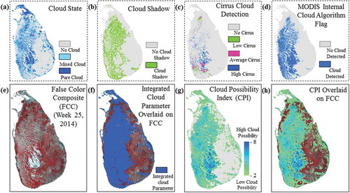
At first, the spatial distribution of different classes of four cloud-related parameters are created for all the composites. Example results for the 25^th week in 2014 over Sri Lanka is provided in Figure 4. One can see cloud related noise information in all four parameters (Figures 4a, 4b, 4c, 4d) and hence simply considering one parameter as a cloud mask would mislead. If all four-parameters are combined with equal consideration as a cloud (Figure 4f) then it would only provide the major noise distribution but not the intensity. Therefore, each attribute class is rated (Table 1) and then summed to derive Cloud Possibility Index (CPI) (Figure 4g). The value of CPI ranges between 0 and 8, where the value “0ʹ represents the no cloud or relatively high-quality pixel, and the value 8ʹ represents high cloud possibility or very low-quality pixel.” The distribution and concentration of cloud can be seen in the central region of Sri Lanka (Figure 3e). It can be seen in CPI (Figure 4g) that majority of the area provides reliable cloud information when compared with False Colour Composite (FCC) (Figures 4e and 4h).

Figure 4.  Spatial distribution of cloud-related parameters over Sri Lanka (25th composite of h25v08 and h26v08 MODIS tiles).

3.2. Evaluation of CPI for noise identification

The simple CPI-based threshold (CPI ≥2) is expected to be effective to identify noisy NDVI value. However, in certain cases disagreement is observed as high NDVI values are also detected as high noise and vice versa due to uncertainty in MODIS quality flag which conforms the observation of the study carried out by Letu et al. (2014). If those values are considered as noise, the annual profile pattern as well as growth cycle rhythm may be incorrectly extracted, and hence additional five different thresholds (Eqn. 2 and Table 2) are evaluated to correctly identify the actual noisy value.

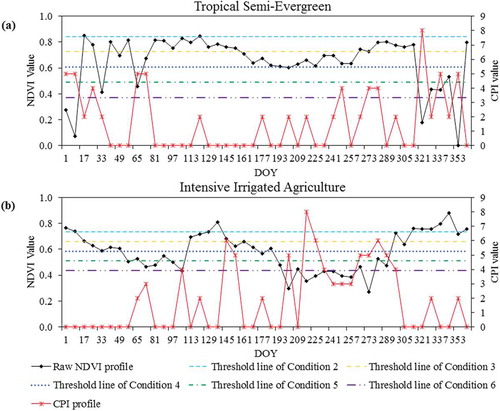
Figure 5 Depicts the graphical concept of threshold in different condition for natural vegetation (Figure 5a) and agriculture (Figure 5b). For the natural vegetation (Figure 5a), the total number of noisy values (i.e. noise count) identified by the TBC 1 is 24 (around 50%) out of 46 input NDVI data points. However, when the NDVI threshold value decreased from high to low (from TBC 1 to TBC 6), the noise count has also gradually decreased from 24 to 4. For agriculture (Figure 5b), TBC 2 and TBC 3 are not helpful in noise reduction, as all the data fell within the threshold range. The condition having a lower threshold, i.e. TBC 5 and TBC 6 is found effective to remove major noisy NDVI value (i.e. lower NDVI value with CPI ≥ 2) correctly. However, any TCF threshold greater than 1 and less than −1 will provide result as same as TBC 1 or raw data.

Figure 5. Graphical example of different threshold level over (a) natural vegetation and (b) agriculture.

3.3. Effect of CPI based reconstruction on different land cover

The NDVI and CPI variations over different land cover features are studied further, and the land cover map (GLC2000) is used for this purpose. Four different vegetation classes (evergreen, semi-evergreen, moist deciduous and dry deciduous) and two agriculture classes (rain-fed crop [single growing cycle], intensive irrigated crop [double and triple growing cycle]) in Sri Lanka are also selected. To ensure the reliability of the chosen pixel, the GLC2000 data is verified with Google Earth image to avoid multi-class mixing area and the samples are collected in the middle of the homogeneous cluster. The higher CPI value is not necessarily related to true noise as the pattern and intensity of noise varies with land use and land cover type. Figure 6 provides the vegetation class-wise graphical illustration of seven smoothed time-series NDVI profiles (six smoothed profiles from six TBC-based reconstructed NDVI data and one smoothed profile based on raw NDVI data). All the seven-profiles has responded differently in terms of growth rhythm depending on the land use and land cover (LULC) class, magnitude of NDVI value, quantity and intensity of cloud noise (CPI value), and defined threshold. The smooth profile from raw NDVI data is compared with the other six profiles, and it has resulted in wrong estimation (e.g., having multiple growing cycles instead of a single growing cycle) of annual growth patterns in the cases of natural vegetation classes (tropical evergreen [Figure 6a], tropical semi-evergreen [Figure 6b], tropical moist deciduous [Figure 6c] and tropical dry deciduous [Figure 6d]).

Figure 6. Raw NDVI and smoothed NDVI profile (based on different conditions) for (a) tropical dry evergreen forest, (b) tropical moist semi-evergreen forest, (c) tropical moist deciduous forest, (d) tropical dry deciduous forest, (e) rain-fed crop (single growing cycle), (f) intensive irrigated crop (double growing cycle), and (g) intensive irrigated crop (triple growing cycle).

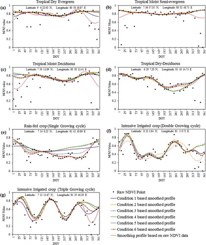
For natural vegetation, though all six conditions have provided reliable results in terms of annual vegetation growth pattern and annual growing cycle, TBC 3 [] based smoothing profile is observed as the most reliable (having single growing cycle and closely matching the non-noisy raw NDVI value) for all cases. However, for agriculture classes TBC 5 and 6 provides maximum agreement when compared with non-noisy raw NDVI value.

3.4. Simulation based performance evaluation of reconstruction model

Sample time-series NDVI data sets with different percentage of random data dropout (10%, 20%, 30%, 40%, and 50% of gaps) are created (i.e. 5 different sets each having 100 annual profiles) using a reference smoothed NDVI profile. Then these 500 profiles are reconstructed using Eqn. 5 and smoothed using DFT. Finally, RMSE, MAE, MBE and MAPE are calculated. Table 3 provides the details about the different error measurements. Figure 7 illustrates the histogram of MBE error distribution from different % of data gaps. It can be observed that at each gap level the average RMSE, MAE, MBE and MAPE values obtained by the model is close to zero. Overall it is revealed that the proposed approach can be used to reconstruct time-series data in a reliable manner.

Table 3. Reconstruction model error statistics (RMSE, MAE, MBE, and MAPE) for five gap levels (10%, 20%, 30%, 40%, and 50%).

	Descriptive statistics	% Data gap
		10%	20%	30%	40%	50%
RMSE	Min	0.0023	0.0017	0.0053	0.0053	0.0103
	Max	0.0229	0.0281	0.0273	0.0351	0.0423
	Mean	0.0215	0.0219	0.0227	0.0234	0.0252
	SD	0.0026	0.0029	0.0024	0.0028	0.0037
MAE	Min	0.0001	0.0009	0.0011	0.0016	0.0012
	Max	0.0044	0.0106	0.0098	0.0158	0.0199
	Mean	0.0014	0.0025	0.0035	0.0045	0.0064
	SD	0.0009	0.0013	0.0015	0.0022	0.0031
MBE	Min	−0.0022	−0.0039	−0.0041	−0.0043	−0.0068
	Max	0.0027	0.0069	0.0054	0.0104	0.0149
	Mean	0.0000	−0.0002	0.0001	−0.0001	0.0000
	SD	0.0008	0.0015	0.0019	0.0025	0.0035
MAPE	Min	0.0086	0.1100	0.1459	0.2118	0.1604
	Max	0.6408	1.5738	1.4422	2.3581	3.0005
	Mean	0.1983	0.3539	0.4963	0.6249	0.8878
	SD	0.1294	0.1954	0.2239	0.3297	0.4720

Figure 7. Mean bias error (MBE) distribution and error statistics from simulated annual profiles with (a) 10% gap, (b) 20% gap, (c) 30% gap, (d) 40% gap, and (e) 50% gap.

3.5. Regional applications

Annual growth rhythm of vegetation is characterized through time-series NDVI data. The biophysical and growth information such as biomass, timing of greening, browning and peak growth and stress in vigor can be extracted using time-series NDVI, but the reliability largely depends on the quality or number of non-noisy occurrence of NDVI value in a year. In this regard, the study wanted to test the appropriateness of the method for such thematic applications at a regional level.

3.5.1. Impact of cloud correction on vegetation growth

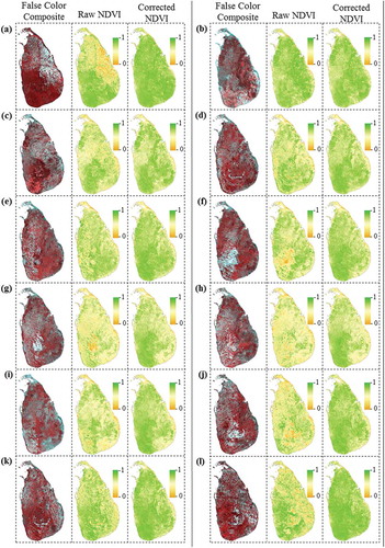
The graphical comparison of MODIS FCC (second week of each month), computed raw NDVI and TBC 3-based (as an example case) smoothed NDVI are shown in Figure 8. Sri Lanka experiences two rainy season due to its geographical setup and as a consequence, cloud cover can be observed in most of the months (January [Figure 8a] to December [Figure 8l]). The frequent cloud cover affects the data quality and as a result lower magnitude of NDVI value is observed in the cloud affected area.

Figure 8. Spatial distribution of MODIS FCC, raw NDVI and corrected NDVI (based on TBC 3) of different composites of different months: (a) 2nd (2nd week of January), (b) 6th (2nd week of February), (c) 10th (2nd week of March), (d) 14th (2nd week of April), (e) 17th (2nd week of May), (f) 21st (2nd week of June), (g) 25th (2nd week of July), (g) 29th (2nd week of August), (i) 33rd (2nd week of September), (j) 37th (2nd week of October), (k) 40th (2nd week of November), and (l) 44th composite (2nd week of December).

We have extracted information about the NGC for the year 2014 using all six conditions (using CPI & NDVI) as well as using raw NDVI data (i.e. without CPI-based noise correction). To evaluate the performance of different conditions over the forest and agricultural area, GLC30 LULC data is degraded (based on majority function) to 500 m first and then based on percentage of mixing (within 500 m × 500 m), we have selected samples of the heterogeneous and homogeneous core area. We have checked the accuracy of extracted NGC information based on (a) samples over heterogeneous cluster of natural vegetation (440 samples) and agriculture (200 samples), (b) samples over homogeneous clusters of natural vegetation (183 samples) and agriculture (186 samples). At each sample, we examined annual smoothed NDVI profile to identify the growing cycle information and labeled it accordingly, which is further considered as reference data. The results based on 6 different conditions (TBC 1 to TBC 6) are compared with reference sample data to evaluate their noise correction performance.

Generally, natural vegetation is characterized by a single growing cycle. The maximum percentage of correctly estimated single growing cycles under heterogeneous sample pixels is observed in TBC 3 (95.37%), TBC 2 (94.44%), and TBC 1 (93.75%) (Table 4). The highest percentage of correctly estimated single growing cycle is observed under homogeneous sample pixels in TBC 1 (98.36%), TBC 2 (96.17%), and TBC 3 (96.17%) (Table 4). The results using non-cloud corrected NDVI data has produced an agreement of 52.78% and 58.47% under heterogeneous and homogeneous locations, respectively. The spatial distribution of growing cycle information extracted from different conditions-based smoothed profile for natural vegetation and agriculture are presented in Figures 9 and 10, respectively.

Table 4. Sampling based performance evaluation of different TBCs results in estimating number of growth cycles in natural vegetation.

Result based on different conditions	Heterogeneous sampling			Homogeneous sampling
	Total number of samples	Single growing cycle		Total number of samples	Single growing cycle
		Quantitative estimation	% correctly estimated pixel		Quantitative estimation	% correctly estimated pixel
TBC 1	440	405	93.75	183	180	98.36
TBC 2		408	94.44		176	96.17
TBC 3		412	95.37		176	96.17
TBC 4		386	89.35		172	93.99
TBC 5		349	80.79		160	87.43
TBC 6		318	73.61		139	75.96
Without CPI		228	52.78		107	58.47

Figure 9. The spatial distribution of extracted growing cycle in forested region based on smoothed results from (a) TBC 1, (b) TBC 2, (c) TBC 3, (d) TBC 4, (e) TBC 5, (f) TBC 6, and (g) without CPI.

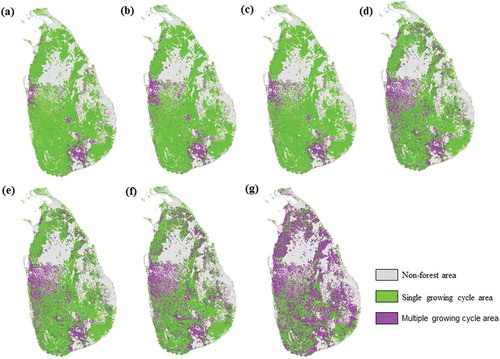
Figure 10. The spatial distribution of number of growing cycle in agricultural region based on smoothed results from (a) TBC 1, (b) TBC 2, (c) TBC 3, (d) TBC 4, (e) TBC 5, (f) TBC 6, and (g) without CPI.

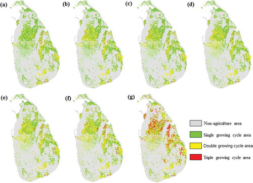
Rain-fed agriculture is characterized by single growing cycles as the water availability depends upon the rainy season whereas irrigated agriculture is characterized by single to multiple growing cycles due to water availability throughout the year. The maximum overall accuracy is observed in TBC 6 (87.5% and 81.18%) followed by TBC 5 (79% and 76.88%), and TBC 4 (78.5% and 72.58%) under heterogeneous and homogeneous sampling scheme, respectively (Tables 5 and 6). However, the least agreement is observed when raw NDVI (without using CPI) is used (62.5% for heterogeneous and 50.54% for homogeneous).

Table 5. Performance evaluation of different TBCs result based on number of growth cycles in heterogeneous agriculture samples.

Result based on different conditions	Single growing cycle			Double growing cycle			Triple growing cycle			Overall accuracy
	Number of sample pixel		% of correctly estimated pixels	Number of sample pixel		% of correctly estimated pixels	Number of sample pixel		% of correctly estimated pixel	Number of sample pixel		% of correctly estimated pixels
	Observed	Estimated		Observed	Estimated		Observed	Estimated		Observed	Estimated
TBC 1	83	76	91.57	102	58	56.86	15	7	46.67	200	141	70.5
TBC 2		73	87.95		72	70.59		8	53.33		153	76.5
TBC 3		77	92.77		64	62.75		7	46.67		148	74
TBC 4		73	87.95		75	73.53		9	60.00		157	78.5
TBC 5		68	81.93		81	79.41		9	60.00		158	79
TBC 6		71	85.54		89	87.25		15	100.00		175	87.5
Without CPI		34	40.96		76	74.51		15	100.00		125	62.5

Table 6. Performance evaluation of different TBCs result based on number of growth cycles in homogeneous agriculture samples.

Result based on different conditions	Single growing cycle			Double growing cycle			Triple growing cycle			Overall accuracy
	Number of sample pixel		% of correctly estimated pixels	Number of sample pixel		% of correctly estimated pixel	Number of sample pixel		% of correctly estimated pixels	Number of sample pixel		% of correctly estimated pixels
	Observed	Estimated		Observed	Estimated		Observed	Estimated		Observed	Estimated
TBC 1	76	66	86.84	103	46	44.66	7	0	0.00	186	112	60.22
TBC 2		64	84.21		64	62.14		1	14.29		129	69.35
TBC 3		70	92.11		57	55.34		2	28.57		129	69.35
TBC 4		70	92.11		63	61.17		2	28.57		135	72.58
TBC 5		66	86.84		73	70.87		4	57.14		143	76.88
TBC 6		65	85.53		79	76.70		7	100.00		151	81.18
Without CPI		34	44.74		54	52.43		6	85.71		94	50.54

Zhou et al. (2012) has recommended different thresholds for different vegetation types. The findings from the current study also confirms that single threshold is not appropriate for noise reduction, and maximum accuracy is obtained only when different thresholds (i.e. TBC 2 and TBC 6) are used in the reconstruction process for natural vegetation and agriculture pixels.

3.5.2. Impact of cloud correction on drought monitoring

According to FAO (2015) report, there was no drought during 2014–15 Maha season in Sri Lanka. But if we use noisy NDVI then it might reveal wrong drought condition. Hence, we wanted to test the results from drought perspective. To evaluate the impact of cloud correction (based on proposed approach) on agriculture drought monitoring, we have used TBC 6 (as it resulted in maximum accuracy) for noise elimination for all the 14-years (2001 to 2014) time-series NDVI data and VCI is computed for each 8-day composite from July to August in 2014. It is important to note that the lower values of VCI not always represent the drought scenario as it can also occur during onset and end of cropping season if seasonal shift in cropping happens over the time. And hence we used VCI only during crop growth period (2nd week of July 2014 to 3rd week of August 2014) as an example case for this discussion.

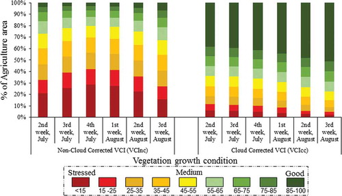
Cloud corrected and non-cloud corrected NDVI data are used to compute two different VCI (i.e. cloud corrected VCI termed as VCI_cc and non-cloud corrected VCI termed as VCI_nc) for comparative evaluation purpose. Week-wise spatial distribution of VCI_cc and VCI_nc over agriculture region of Sri Lanka is illustrated in Figure 11, and one can see the consistent stress condition in VCI_nc based results whereas VCI_cc shows normal correct growth condition. Finally, VCI values are grouped into nine different drought classes according to FAO (2016). Figure 12 represents the class-wise percentage of agriculture area extracted using six continuous weeks VCI_cc and VCI_nc data. As per VCI_nc data, more than 50% of agriculture area is found to be under severe drought during cropping season whereas there was no actual drought on ground, and the area estimated using VCI_cc data has correctly revealed the healthy ground condition over 85% of the area. Observation from Figures 11 and 12 clearly indicates that drought monitoring using non-cloud corrected NDVI would mislead drought quantification and hence affect decision-making especially at the crucial cropping period.

Figure 11. Spatial distribution of cloud corrected VCI and non-cloud corrected VCI over Sri Lanka for (a) 2nd week of July, (b) 3rd week of July, (c) 4th week of July, (d) 1st week of August, (e) 2nd week of August, and (f) 3rd week of August in 2014.

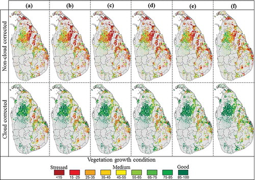
Figure 12. Class-wise % of agriculture area extracted using cloud-corrected VCI and non-cloud-corrected VCI over Sri Lanka for six continuous weeks from 2nd week of July to 3rd week of August, 2014.

4. Conclusion

The study has found that using the cloud-related parameters from MODIS state flag as absolute noise has resulted in overestimation of clouds. In this study, we have proposed and tested simple reproducible procedures to map cloud presence (CPI) based on MODIS quality parameters and to detect noise in NDVI time-series, and for gap filling and reconstruction procedure (before applying Fourier smoothening). The performance of the reconstruction model has been evaluated based on five different percentage levels (10%, 20%, 30%, 40%, and, 50%) of gap simulation, and the model is found to be effective based on four statistical error measures (i.e. RMSE, MAE, MBE, and MAPE).

The study has checked the usability of the approaches for vegetation phenology and drought applications. Under vegetation phenology, the study has tested the detection accuracy of all the TBCs for their correctness in revealing number of growing cycle information in natural vegetation (>90% accuracy) and agriculture area (>80% accuracy) based on 100 s of homogeneous and heterogeneous sample points. It is observed that utilizing CPI alone has improved the NGC detection accuracy from 50–60% to >90% in all the homogeneous natural vegetation, and from 45% to 87% in single-cropping area. However, for heterogeneous pixels, CPI alone is not enough to identify noise especially in the cases of double and triple cropping regions. Different TCF based additional checks have revealed that TBC 2 & 3 are better choice for noise elimination in natural vegetation, and TBC 5 & 6 for agriculture. The study also has analyzed the effect of different approaches for drought assessment during crop growing time (i.e. 2014 Maha season) in Sri Lanka. The total area falling under drought categories based on non-cloud corrected data is observed to be varying between 40 to 56% during crop growth period, and on the other hand results from cloud corrected data has correctly revealed the area between 9 and 18%. The study has found that drought monitoring using non-cloud-corrected data (without CPI) overestimates the intensity, spatial distribution, and magnitude of drought in the study area though there was no major drought. The study recommends that the proposed approaches may further be tested over different altitudinal and climatic conditions across the globe.

Acknowledgment

The authors would like to appreciate and acknowledge NASA MODIS team for freely sharing the time-series satellite data and IWMI for the time to time necessary support. Thanks to all the anonymous reviewers whose critical comments and suggestions have greatly helped in improving the manuscript.

Disclosure statement

No potential conflict of interest was reported by the authors.