Updating land cover automatically based on change detection using satellite images: case study of national forests in Southern California

Abstract

Observing dynamic change patterns and higher-order complexities from remotely sensed images is warranted, but the main challenges include image inconsistency, plant phenological differences, weather variations, and difficulties of incorporating natural conditions into automatic image processing. In this study, we proposed a new algorithm and demonstrated it by producing 2002–2008 and 2010 land-cover maps in heterogeneous Southern California based on an existing 2009 land-cover map. The new algorithm improves the baseline land-cover map quality by discarding potential bad land-cover pixels and dividing each land-cover type into several subclasses. Time series Landsat images were used to detect changed and unchanged areas between baseline year and target year t. Subsequently, for each individual year t, each pixel that was identified as unchanged inherited the baseline classification. Otherwise, each pixel in the changed areas was classified by a similar surrogate majority classifier. The demonstration results in Southern California showed that the land-cover temporal pattern captured the observed successional stages of the ecosystem very well. The accuracy assessment had an overall classification accuracies ranging from 81% to 86% and overall kappa coefficients ranging from 0.79 to 0.83.

Keywords:

• land cover
• update
• time series images
• change detection
• remote sensing

1. Introduction

Land-cover changes affect the biophysics, biogeochemistry, and biogeography of the Earth’s surface and atmosphere, with far-reaching consequences to human well-being (Giri et al. 2013). With the free availability of Landsat images or similar resolution satellite data sources (e.g., SPOT, LISS, AWiFS, CBERS, and Sentinel 2A/2B), large area multi-temporal land-cover monitoring at 30 m spatial resolutions is desired to observe dynamic change patterns and higher-order complexities (Fu, Li, and Pirasteh 2015; Hansen and Loveland 2012; Giri et al. 2013; Verburg, Neumann, and Nol 2011; Han et al. 2015). This process needs to be streamlined and automated (Maclaurin and Leyk 2016). Several large land-cover projects have been conducted for time series monitoring. For example, Vogelmann et al. (2001), Homer et al. (2004), Xian, Homer, and Fry (2009), and Jin et al. (2013) developed US National Land Cover Datasets (NLCD) for different consecutive time periods. Zhang et al. (2014) developed a national land use and land-cover database of China at a 1:100,000 scale for five time periods in the 1980s, 1995, 2000, 2005, and 2008. The United States Department of Agriculture National Agricultural Statistical Service produced an annual cropland datalayer (Johnson & Mueller, 2010). For these different large area land-cover change projects, a considerable amount of methodological variations exist, but documenting time series land-cover changes at regional and global scales still remains quite challenging, because image inconsistency (in terms of spectral coverage, sensor calibration, and atmospheric correction), plant phenological differences, weather variations, and heterogeneous natural conditions create obstacles for producing reliable land monitoring data and information (Giri et al. 2013). Despite so many approaches, supervised methods or slight variations of supervised approaches generally are favored (Chen et al. 2015; Hansen and Loveland 2012).

When ground-truthed labels are available for all the items of the temporal series, the process of temporal updating of land-cover maps can be particularly effective with a supervised approach; however, gathering reliable ground-truthed data for each specific acquisition date is not realistic (Bruzzone and Marconcini 2009). Signature extension, where signatures are extracted from a known feature and used to classify the same feature type located at some distance in time and space from the signature source (Olthof, Butson, and Fraser 2005), can apply a supervised classification to a time series of Landsat scenes given extensive radiometric correction, but the procedure cannot be fully automated due to the dependence on an interpreter throughout the classification process (Maclaurin and Leyk 2016). Bruzzone and Marconcini (2009) proposed a domain adaptation (DA) support vector machine (SVM) approach for automatically updating land-cover maps by using remote-sensing images periodically acquired over the same investigated area; however, ground-truthed labels were required to be available for a reference image. This is also the case for Bahirat et al. (2012) who proposed a DA Bayesian classifier based on maximum a posteriori decision rule (DA-MAP) for updating land-cover maps. Recently, Maclaurin and Leyk (2016) relied solely on remote-sensing imagery and employed a maximum entropy classifier to extract information from one Landsat image using an existing land-cover map, and then reproduced the classification using a Landsat image from a different point in time. When they tested their method for bi-temporal classification in three small study areas (387, 1339, and 1257 km²), they found that increased landscape heterogeneity reduced the land-cover classification accuracy, which was also mentioned by Smith et al. (2003). These indicate that remote sensing alone may not be sufficient and the auxiliary environmental datasets such as elevation and climate might be needed for the land-cover classification over a large complex landscape.

The objective of this article is to propose a new approach to process remote sensing and ancillary geospatial datasets for automatically updating time series land-cover databases over a large complex landscape. This kind of algorithm is also critical for the US Department of Agriculture Forest Service Forest Inventory Analysis (FIA) programs. For the FIA program, it was suggested that the satellite imagery be classified into homogeneous classes as strata for reporting purpose (McRoberts, Nelson, and Wendt 2002). NLCD was investigated as the basis for stratifications; however, there were two problems: First, the NLCD classification was not designed for forest inventory estimation and therefore did not satisfy FIA precision standards. Second, the NLCD updating frequency of 5–10 years could not meet the FIA plot measurement cycle of 5 years for much of the United States. Thus, the classifications would always be out of date (McRoberts, Nelson, and Wendt 2002). Due to these reasons, the regional FIA programs may find it necessary to produce their own classifications. Nevertheless, approximately 125 Landsat TM scenes need to be classified over each 5-year FIA measurement cycle for a regional FIA program (McRoberts, Nelson, and Wendt 2002). Especially, the national forests in the Southern California have a great diversity of geologic, topographic, and ecological characteristics. Frequent land disturbances (mainly wildfires) occur in this area and have been a major factor in the survival of its vegetation over much of its ancient to recent history. Additional stressors include the occurrences of seasonal and multi-year drought episodes followed by large bark beetle outbreak. These ecosystem disturbances associated with a heterogeneous landscape create highly dynamic land-cover change conditions that require frequent updates to land-cover classification maps in order to understand the complexity of this landscape. The land-cover map for year 2009 existed, but annual land-cover maps from 2002 to 2010 in and around the Cleveland National Forest, the San Bernardino National Forest, and the Angeles National Forest in Southern California are desired for monitoring.

Bearing these aforementioned in mind, we aimed to use these three national forests as a case study to report a new algorithm on producing time series land-cover maps. The new algorithm was proposed to update annual land cover from an existing baseline land-cover map. Temporal updating of land-cover datasets is usually based on detecting areas that have changed since the previous release and reclassifying these areas (e.g., Jin et al. 2013). Our algorithm is based on a conventional change detection approach to identify changed and unchanged area, but an innovative similar surrogate majority classifier (SSMC) is proposed to classify the images in an iterative manner. SSMC has three new features. First, SSMC uses majority voting from similar pixels within unchanged areas; this concept has not been reported for land-cover classification. Second, the training samples for SSMC are from an existing land-cover map, and no additional effort is needed for gathering reliable ground-truthed data as training data. Third, not only remote-sensing images but also auxiliary geospatial data (e.g., elevation, aspect, and ecoregion) can be assimilated. We incorporated the algorithm into a tool to automate the processing, and we demonstrated it in the three national forests in Southern California.

2. Study area and datasets

The area of interest (enclosed by the black polygon of Figure 1) encompasses the Angeles, San Bernardino, and Cleveland National Forests as well as surrounding private, Native American, and government lands. A Mediterranean climate, driven in part by the North Pacific subtropical high pressure zone, typifies the area’s climate with cool moist winters and hot dry summers. Elevation in the target area ranges from 10 to 3505 m and slopes vary from flat to very steep. According to the PRISM Climate Data records of 1950–2010 (http://www.prism.oregonstate.edu/), temperatures during the coldest months can range from −6°C to 23°C, with snow typically occurring above about 1830 m, and temperatures during the warmest months can range from 9°C to 42°C. Precipitation can vary from 0 to 29 mm during the driest months and 10–225 mm during the wettest months. In forest and woodland areas of low to middle elevations, conifer species can dominate the landscape either singularly or in combinations. At the highest elevations, subalpine conifers may be present. In addition, many fires have occurred in this ecosystem (see Figure 1).

Figure 1. Study area of Southern California is enclosed by the black polygon. Background images are Landsat5 R5G4B3 composites on 5 July 2009, 14 July 2009, and 27 May 2009 for Path41/Row36 (blue), Path40/Row36 (red), and Path40/Row37 (green), respectively. Fire year and location during 1992–2010 are identified (source: Monitoring Trends in Burn Severity, http://www.mtbs.gov/). For full colour versions of the figures in this paper, please see the online version.

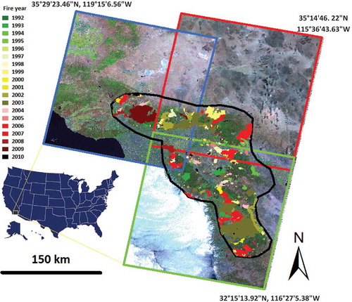
Before this project implementation, an existing land-cover classification map had been produced for the year of 2009 with an overall accuracy of 89% (Figure 2). Our project’s aim was to update land-cover changes for the retrospective years 2002 through 2008 and prospectively for 2010. Since the study area is covered by three Landsat 5 footprints indicated by the red, blue, and green rectangles (see Figure 1), Landsat 5 imageries generated from the Landsat Ecosystem Disturbance Adaptive Processing System (LEDAPS) algorithm (Masek et al. 2006) were collected for this project (Table 1). These images were selected because (a) they had little cloud and snow cover; (b) they were acquired in the months when the vegetation showed distinguishing variation; (c) they were all acquired around a similar acquisition date, thereby minimizing the weather and phenology influence; and (d) they were from the same sensor and consistent. Three derivative indices were also calculated for these Landsat 5 images, including moisture stress index (MSI = band 5/band 4), normalized difference vegetation index (NDVI = (band 4 – band 3)/(band 4 + band 3)), and normalized burn ratio (NBR = (band 4 – band7)/(band 4 + band 7)). In addition, we downloaded Monitoring Trends in Burn Severity (http://www.mtbs.gov/) data; we compiled GIS datasets of ecoregions, national forest boundaries, elevation, and aspect. These datasets were empirically chosen based on our local knowledge of this ecosystem and preprocessed so that they can be properly used for similarity determination (Figure 3).

Table 1. Landsat 5 acquisition dates for the three paths/rows.

	2002	2003	2004	2005	2006	2007	2008	2009^a	2010
Path41/Row 36	16 June	5 July	5 June	8 June	10 May	14 June	31 May	5 July	6 June
Path40/Row36	24 May	27 May	14 June	3 July	4 June	9 July	9 June	14 July	30 May
Path40/Row37	24 May	27 May	14 June	1 June	4 June	9 July	9 June	27 May	30 May

^a Landsat acquired in 2009 were taken as the baseline images.

Figure 2. Baseline land-cover classification data in 2009.

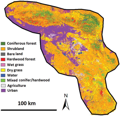
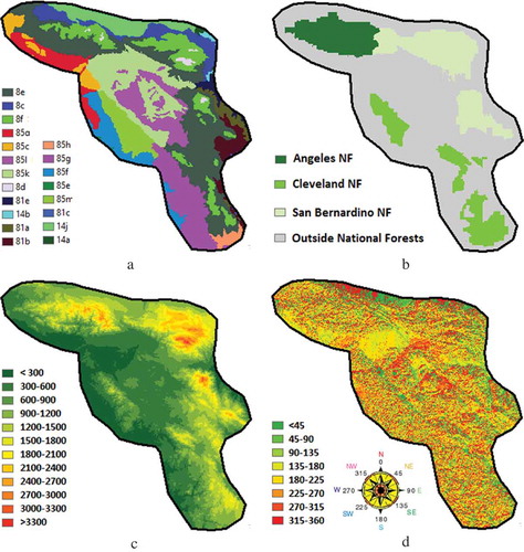
Figure 3. Natural condition zones used for the similar surrogate majority classification with priority ordered by (a) 20 level IV ecoregions (see codes at http://www.epa.gov/); (b) 4 national forest zones; (c) 12 elevation (in meters) classes; and (d) 8 aspect (in degrees) classes.

3. Methodology

3.1. Overview

We used the 2009 classification (Figure 2) as a baseline to produce land-cover data for a specific year t (i.e., 2002–2008, 2010). The potentially misclassified or mixed pixels in the 2009 baseline land-cover map were discarded as much as possible and each land-cover class was divided into three subclasses. Then, we detected the changed and unchanged areas between 2009 and year t. For each year t, the land-cover classification in an unchanged area was inherited from the baseline 2009 classification. However, for each changed pixel, the land-cover classification was determined as the majority of its “similar” surrogates from the unchanged areas. A detailed flowchart of this concept, from which the software tool “Automatic Update On Land Cover Database (AutoLCD)” was developed, is illustrated in Figure 4.

Figure 4. Flowchart and conceptual modeling framework of AutoLCD.

3.2. Improving baseline land-cover quality

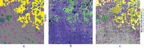
The 2009 classification dataset was a baseline map from which all other annual land-cover products in this project were developed. However, it is very common to find errors in thematic land-cover classifications. Even if the classification is correct, the same class may be composed of spectrally distinguishable objects. For example, a “wetland” class may contain open clear water, contaminated water, marsh, fen, or peatland, which have quite different reflectance values. From a statistics aspect, the misclassified pixels in a specific class usually deviate from the mean and have very low or very high noisy values; therefore, to improve the quality of the 2009 classification dataset for helping the classification in other years, we calculated the mean and standard deviation (Std) for band 3, band 4, and band 5 of the 2009 baseline Landsat data within each individual class. Those pixels that were beyond the range of the [mean ± (n*Std)] were taken as misclassified pixels and discarded from the baseline classification. Here, “n” is chosen by users and 2 was chosen for our study. Further, we used the Iterative Self-Organizing Data Analysis Technique (ISODATA) algorithm (Mather and Koch 2011) to divide each original class into three subclasses. Although some other approaches such as self organizing map (Awad 2010) may be better, ISODATA was adopted here for three reasons. First, it is widely used and well known. Second, it is an unsupervised method avoiding training data selection. Third, ISODATA was already included and easily available in the ArcGIS ArcPy module on which the development of AutoLCD was based. The subclasses were subsequently used for updating annual land cover and finally merged back into the original class. Figure 5 shows the concept of improving the quality of a baseline classification.

Figure 5. An example of improving the baseline land-cover map quality based on the baseline image. (a) Baseline land-cover classification data with five categories; (b) baseline Landsat R5G4B3; and (c) improved classification with each raw class divided into three subclasses after outliers (white pixels) are removed.

3.3. Identify changed and unchanged areas

Our method utilized changed and unchanged areas to update land cover. We incorporated multi-temporal remote-sensing data sets to detect change. For each pixel, the change detection was based on the range (Equation (1)) and coefficient of variation (COV, Equation (2)) of that pixel’s values (in terms of Landsat metrics) over time:

(1)

(2)

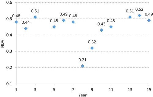
The “Range” is defined as the difference between the maximum (Max) and minimum (Min) values; it can depict the absolute magnitude of land surface change. The “COV” is defined as the ratio of the standard deviation (Std) to the mean; it can quantify the magnitude of relative change, with a greater COV value indicating a higher degree of change. To better understand the “Range” and “COV” definitions, we illustrate their concepts using Figure 6 where the range is 0.31 and COV is 0.196.

Figure 6. Example of a pixel’s normalized difference vegetation index (NDVI) over 15 years, where year 4 and year 12 are absent due to cloud and shadow contamination. Maximum and minimum NDVI values are 0.52 and 0.21, respectively, resulting in a range of 0.31. Mean and standard deviation of these NDVI values are 0.445 and 0.087, respectively, resulting in a coefficient of variation (COV) of 0.196. The missing values are ignored during these calculations.

We used the criteria “Range ≥A or COV >B” to aggressively determine the changed areas. Here, A and B are two empirical threshold values so that we would overestimate rather than underestimate the changed areas. In this study, we chose three Landsat metrics – NDVI, MSI and NBR – to separately identify the changed areas, because these three metrics are sensitive to vegetation change caused by the disturbances from drought, fire, and beetles (Tucker 1979; Cocke, Fulé, and Crouse 2005; Meddens and Hicke 2014). We combined these three separate changed area datasets into a map called maximum changed area (MCA).

MCA could depict the pixels where the land cover was possibly changed within the whole period. However, MCA could not depict the annual area of change. Therefore, the creation of an annual changed area (ACA) map was needed. We accomplished this through two steps. First, we compared each year’s Landsat NDVI, MSI, and NBR with the corresponding 2009 Landsat indices and identified the changed areas even more aggressively (through A and B values) with a similar approach of MCA detection (i.e., based on Equations (1) and (2)), but the changed areas were constrained within MCA. Second, once a pixel was determined to be changed at year t, this pixel was automatically assigned to be changed at year t + 1 until the last year of the time series. The automatic change assignment from t to t + 1 was adopted because the change detected in year t might not be detected in t + 1. For each year t, the remaining pixels that were not detected by ACA were considered to be unchanged areas.

3.4. SSMC

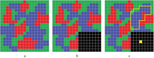
For each target year t, if an area was identified as unchanged, the 2009 baseline classification could be used directly for the target classification. However, if a pixel was detected as a changed pixel or if the pixel was determined as misclassified pixel in Section 3.2, its classification was determined from the majority of similar pixels occurring in the unchanged areas. Figure 7 illustrates the concept of this SSMC in which the black area is identified as a changed area. The areas that are identified as unchanged inherit their land-cover values from the baseline classification, as represented in Figure 7b where they have the same red, green, and blue values as in Figure 7a. On the other hand, the yellow pixel in Figure 7c, representing a changed pixel, has a total of 36 similar pixels, in which 4 are green, 3 are red, and 29 are blue. The majority of these similar pixels is blue, resulting in the yellow pixel receiving the “blue” land-cover classification. This process is repeated for every pixel in the changed area. More details of the SSMC follows.

Figure 7. Basic concept of the classifier. (a) Baseline land-cover classification data where red, green, and blue indicates different land-cover values; (b) black areas indicate changed areas, while the rest are unchanged areas; (c) “similar” surrogates of the yellow pixel are enclosed by the yellow polygon. The majority of these “similar” pixels, which in this case is blue, are deemed as the land-cover value for the yellow pixel.

3.4.1. “Similarity” determination

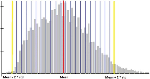
The first step of the “similarity” determination, which was previously reported in Huang et al. (2016), was based on the remote-sensing imagery from year t. We chose the Landsat bands 3, 4, 5, and 7 due to their sensitivity to land surface change. The mean and standard deviation of each individual band were calculated from all pixels. Then each band was partitioned into 10 bins with the upper and lower values of [mean ± 2Std] as references (see binning concept in Figure 8). For a changed pixel waiting for land-cover class assignment, only those unchanged pixels in the same binned group were qualified to be candidate surrogates.

Figure 8. Concept of binning. Mean ± 2Std are the upper and lower limits (shown in yellow). The metric is binned into n groups where n is the number provided by users (in this case, n = 23).

The second step of “similarity” determination was based on natural and social conditions. For remote-sensing classification, it is well known that the landscape heterogeneity in terms of climate, topography, soil, moisture, vegetation, and even land use hampers the accuracy improvement. Because of heterogeneity, similar remote-sensing metrics may indicate quite different land cover while dissimilar remote-sensing metrics may indicate the same land cover; therefore, landscape heterogeneity needs to be considered in land-cover classification, especially when terrain is quite variable. For a changed pixel waiting for land-cover class assignment, only those unchanged pixels in the same environmental conditions were qualified to be candidate surrogates.

By combining all groups from remote-sensing bands and environmental conditions mentioned above (i.e., with the ArcGIS “combine” function), only the unchanged pixels in the same unique group were selected as surrogates.

3.4.2. “Majority” constraints

The target pixel received the value of the class with the majority of “similar” surrogates. This step was applied to each individual pixel in the changed areas. However, a simple “majority” approach may have two issues. First, if the number of the candidate pixels (i.e., the sum of red, green, and blue pixels enclosed by the yellow polygon in Figure 7c) was very small (e.g., only 1 or 2 pixels), then the confidence level of the classification would be low, because any errors contained in these few pixels would be propagated to the target classification. Therefore, we defined a lower threshold of 20 to be the minimum number of candidate pixels allowed for the SSMC to be performed. Second, assuming that there were enough candidate pixels for the SSMC (e.g., 100 pixels) to be executed, but the percentage of the pixels in the majority class compared to the total number of candidate pixels was low, then the confidence level of the classification would also be low. To illustrate this, assume there are 100 candidate pixels for the yellow pixel in Figure 7c, of which 33 are red, 33 are green, and 34 are blue. The majority class would be blue, but in this case, the estimation is not reliable, as the percentage is only 34%. To solve this issue, we selected a lower threshold of 60% to define a minimum acceptable percentage for the SSMC to be performed. Both the threshold of a minimum number of candidate pixels and the threshold of a minimum acceptable percentage were thereby used to improve the reliability of the classification.

3.4.3. “Majority” iteration

During the SSMC, there were many constraints, including mathematically allocating bins, applying natural/social conditions, determining a minimum pixel number, and determining a minimum percentage, as mentioned above. It was possible that the SSMC could not be performed for a changed pixel because there were not enough candidate surrogates meeting all these conditions. To solve this problem, we created an order of priority for the environmental condition constraint, where “ecoregion > elevation > aspect > national forest zone” (see Figure 3). This meant that “ecoregion” was the most important natural condition, whereas “national forest zone” was the least important natural condition.

Initially, the 4 Landsat bands (i.e., bands 3, 4, 5, and 7 that were already divided into 10 bins each), 20 ecoregions, 12 elevation classes, 8 aspect classes, and 4 national forest zones theoretically separated the study area into 10 × 10 × 10 × 10 × 20 × 12 × 8 × 4 = 76,800,000 unique combination groups. Then, the SSMC was applied to classify the image. If the classification could not be performed for a pixel due to insufficient candidate surrogates, the least important constraint (“national forest zone”) was discarded, which would separate the study area into 10 × 10 × 10 × 10 × 20 × 12 × 8 = 19,200,000 unique combination groups. The SSMC was then applied to classify the remaining unclassified pixels of the image. This was repeated until the most important “ecoregion” was ignored, resulting in 10 × 10 × 10 × 10 = 10,000 unique combination groups. If the SSMC still could not be produced for a pixel, we reduced the number of remote-sensing bins from 10 to 5 and repeated the above procedure.

From the aforementioned process, we can see the classification was conducted in an iterative manner. It started with a high number of bins and all environmental condition constraints for classification, and then iteratively proceeded to classify the remaining pixels with fewer bins and fewer condition constraints.

3.4.4. Incorporating heuristic rules into “majority” classification

Heuristic rules are very common in remote-sensing classifications and knowledge of the project area can substantially improve the land-cover classification, as demonstrated in previous examples (e.g., Vogelmann et al. 2001; Homer et al. 2007; Xian, Homer, and Fry 2009; Jin et al. 2013; Chen et al. 2015). In this study, the following heuristic rules were incorporated into our tool specifically for our study area to improve the classification:

1. In high mountains where elevations was >1500 m, and the NDVI value was >0.30, pixels should not be classified as bare land or water.

2. If the 2009 classification was agriculture or urban and the NDVI change (2009 vs. year t) was <0.3, the classification for year t should remain the same as the 2009 classification.

3. Within burned areas where the fire severity was rated as “medium” or “high” intensity, the following rules apply:

1. In the first postfire year, only bare land (where NDVI was ≤0.28) or grassland (where NDVI was >0.28) were allowed as land-cover types.

2. In the second postfire year, only bare land (where NDVI was ≤0.28), grassland (where NDVI was >0.28 and <0.37), or shrubland (where NDVI was ≥0.37) were possible land-cover types.

3. In the third postfire year, if NDVI was ≤0.28, pixels were classified as bare land; if NDVI was >0.28, pixels were classified as shrubland.

4. If the fire occurred less than 10 years ago, no conifer cover type was assigned;

5. If the 2009 classification was not a hardwood or a conifer/hardwood mixed cover type, the same area in previous years (2002–2008) was not to be classified as a hardwood or conifer/hardwood mixed cover type.

4. Results

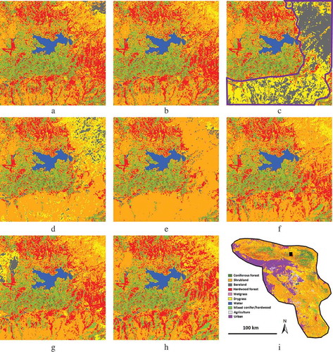
A portion of an annual land-cover map produced in this study is shown in detail in Figure 9, where the right and lower parts of this area were burned on 15 November 2003 (between 2003 and 2004 Landsat acquisition dates). Most of this burned area was hardwood forest and shrubland in 2002 and 2003, but became bare land and grassland in 2004, grassland and shrubland in 2005, shrubland in 2006, and shrubland and sprouting hardwood forest in 2007–2010. This temporal pattern captures the observed successional stages of this ecosystem very well.

Figure 9. Land-cover classes updated with the tool are shown for a small section (9 km × 9 km) of the study area for the years (a) 2002, (b) 2003, (c) 2004, (d) 2005, (e) 2006, (f) 2007, (g) 2008, and (h) 2010. The area burned on 15 November 2003 was roughly marked as purple polygon in (c). The last panel (i) shows the general location of this small section as indicated by the black rectangle.

The land-cover map was evaluated through a conventional accuracy assessment. A total of 284 points, which were compiled from FIA field plots (their locations are fixed but confidential according to US law; and a plot may be surveyed several times during 2002–2010) or visually interpreted from high resolution (1–2 m) images from NAIP and WorldView, were compared with the classification. About 71% of the plots were located in disturbed areas known from data of fires, clear-cuts, plantations, and beetle attacks between 1992 and 2010. Table 2 shows an example of the classification for 2005 with an overall classification accuracy of 83% and an overall kappa coefficient of 0.81. Similar accuracy assessments were implemented for years 2003, 2006, and 2010 when reference data for comparison were available, resulting in overall accuracies of 85%, 81%, and 86% and kappa coefficients of 0.79, 0.80, and 0.83, respectively.

Table 2. Accuracy assessment for 2005 classification.

	Reference points class code
Class code	1	2	3	4	5	6	7	8	9
1 (Coniferous forest)	53	2	0	0	0	0	0	2	0
2 (Shrubland)	2	38	3	2	0	1	0	1	1
3 (Bare land)	0	1	21	0	0	1	1	0	5
4 (Hardwood forest)	2	3	1	39	1	0	0	2	0
5 (Wet grass)	0	0	0	1	4	0	0	0	0
6 (Dry grass)	0	0	1	0	0	10	0	0	1
7 (Water)	0	0	0	0	1	0	13	0	0
8 (Mixed conifer/hardwood)	5	1	0	3	0	0	1	38	0
9 (Urban)	0	0	2	0	0	0	0	0	21
Total	62	45	28	45	6	12	15	43	28
Class code	Reference totals	Classified totals	Number correct	Producer accuracy (%)	Users accuracy (%)
1 (Coniferous forest)	62	57	53	85	93
2 (Shrubland)	45	48	38	84	79
3 (Bare land)	28	29	21	75	72
4 (Hardwood forest)	45	48	39	87	81
5 (Wet grass)	6	5	4	67	80
6 (Dry grass)	12	12	10	83	83
7 (Water)	15	14	13	87	93
8 (Conifer/hardwood mix)	43	48	38	88	79
9 (Urban)	28	23	21	75	91
Total	284	284	237	–	–

Overall classification accuracy = 83%.Overall kappa statistics = 0.81.

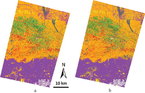
In addition to running a conventional accuracy assessment, we also checked the consistency of the Landsat footprint overlay areas (see Figure 1), where different classifications can be independently produced from different Path/Row datasets (see Table 1). Clearly, if the agreement (i.e., the percentage of the pixels that are classified as the same land cover) is high, it indicates a high robustness. Figure 10 shows the 2002 classification within the overlay area of Path41/Row36 and Path40/Row36. Although separately done, the agreement between land-cover classes was 88.4%. Similar comparisons were conducted for all the Path/Row overlay areas and the agreements between classes ranged from 83.9% to 95.3% (Table 3). In practice, when a pixel in the overlay areas was classified as different land-cover types, the class from the scene with the lowest percentage of cloud pixels within the overlay area will be assigned to the final land-cover map, as the surface reflectance correction of Landsat imagery is likely less effective for scenes with extensive cloud contamination.

Table 3. The percentage agreement within the overlay areas.

	2002	2003	2004	2005	2006	2007	2008	2009	2010
Path40/Row36 vs. Path41/Row36	88.4	88.1	87.4	87.2	87.7	88.0	87.6	86.4	86.5
Path40/Row36 vs. Path40/Row37	91.1	90.2	90.5	86.8	89.5	89.9	89.2	87.3	89.9
Path41Row36 vs. Path40/Row37	95.3	93.7	94.3	83.9	84.1	90.9	86.7	87.7	89.1

Figure 10. Comparison between the overlay area of (a) Path41/Row36 Landsat and (b) Path40/Row36 Landsat for the 2002 classification. The agreement (i.e., the percentage of the pixels that are classified as the same land cover) between the land-cover classes was 88.4%.

5. Discussion

Our goal was to update the land-cover database for Southern California. To address the complex landscape and process many images in an automatic manner, we developed AutoLCD and applied it to our study area. Over a large complex mountainous area covered by three Landsat scenes, this tool automatically produced 8-year annual land-cover maps in a fast fashion, resulting in overall classification accuracies greater than 81% and kappa coefficients greater than 0.79, indicating the potential of applying AutoLCD to other areas. It should be emphasized that previous literatures (Huang et al. 2016, 2017), which focused on continuous variables instead of discrete land-cover classes, had reported similar processes, including (1) defining “similarity” from remote-sensing metrics based on the binning concept, (2) enhancing the “similarity” definition by considering auxiliary geospatial datasets (e.g., elevation, ecoregions), and (3) conducting the computation in an iterative manner. In this demonstrative study, many arbitrary values were used, but AutoLCD allows users to flexibly set up these values according to their own study. For example, how many subclasses are used for dividing each original class; what bands are used for similarity determination; how many standard deviations are used for binning; what auxiliary geospatial datasets are included. However, it is still uncertain if this tool can perform well over other areas. Therefore, testing the robustness over a broader area is advisable to the user. The users need to be aware of three weaknesses and three advantages of AutoLCD.

The first weakness is the baseline land-cover classification data (BLCCD). AutoLCD was designed to update the land-cover database from an existing land-cover map; therefore, it is invalid if the BLCCD is not available. The initial BLCCD should be as accurate as possible, otherwise the errors may persist into the subsequent annual mapping results. The current version of AutoLCD excludes those potentially misclassified pixels from subsequent analysis in order to reduce the risk (see Section 3.2), but we still suggest that the BLCCD be carefully evaluated prior to the AutoLCD application. The importance of baseline land-cover data was also mentioned by Maclaurin and Leyk (2016) who stated that temporal updating of land-cover data relied heavily on the quality of the original land-cover data; therefore, they used a filtering approach to remove likely misclassified training pixels for improvement.

The second weakness is the change detection approach. Change detection is a prerequisite of the SSMC. However, it should be pointed out that there is a shortcoming of change detection in our algorithm. In our study, the input satellite data were anniversary imagery dates or very close to anniversary dates of Landsat images. The only reason for this requirement was to assure that the MCA and ACA could be developed after the effects of sensors, sun angle, seasons, and plant phenological differences could be minimized. The approach of using anniversary imageries to detect MCA and ACA is straightforward, but presently may be out of date since full long time series Landsat data can be accessed. If there is an alternative and robust approach to detect the maximum changed area (MCA) and annual changed area ACA (simply with “1” indicating change and “0” indicating no change) regardless of the type of sensor, the processing level, and the acquisition date, then AutoLCD will not need to rely on optical satellite sensors, image calibration, and anniversary acquisition. In this case, some other sensor data may be used. For example, one may adopt hyperspectral images, which may be superior to Landsat for classification (Awad, Jomaa, and Arab 2014). Therefore, the next step is to integrate the current change detection approach and select or develop a new approach for using AutoLCD (e.g., Roy, Ghosh, and Ghosh 2014; Zhu and Woodcock 2014).

The third weakness is the missing observations. AutoLCD cannot perform accurate land-cover classification, if the area is detected as changed in a specific year but good quality data is lacking (e.g., due to cloud cover). However, the recent advancements in data preprocessing shed light on an effective use of AutoLCD when cloud or shadow occur in the image. For example, Roy et al. (2010) documented the web-enabled Landsat dataset (WELD), which can identify all cloud-free pixels and process Landsat data into seamless weekly, monthly, and seasonal composites. Hermosilla et al. (2015) recently presented a Best-Available-Pixel (BAP) compositing process to generate image composites through a pixel-based approach to enable the production of spatially contiguous, cloud and haze-free, spectrally-consistent, temporal series of proxy surface reflectance composites using Landsat imagery. Despite these three disadvantages, the SSMC, which iteratively utilizes the majority of similar pixels with natural/social conditions taken into account, is the core of AutoLCD and has the following three advantages.

The first advantage is the capability of similar surrogate majority classifier (SSMC) to assimilate multi-sources of remote-sensing data. Radiometric normalization is usually required for large area mapping due to the differences in the sensor, atmospheric conditions, and image calibrations (Hansen and Loveland 2012). However, the SSMC does not require a strict normalization (but note the change detection part still needs one, as aforementioned), because the “similarity” is based on the “binning” concept. Binning has two advantages. First, it is fast. Second, it is conducted in only one image at a time and does not rely on any other data. This advantage enables our approach to take full advantage of different satellite data sources with comparable resolution. For example, if a cloud-free Landsat scene is not available for a specific year, but a SPOT image is available, then we can use SPOT as a surrogate. Similarly, Landsat MSS, Landsat 5, Landsat 7, or Landsat 8 in either digital number or surface reflectance, as well as their derivative metrics (e.g., principal components), can be adopted. It should be noted that only the classifier of SSMC itself has this capability of assimilating different data: the AutoLCD tool relies on a prerequisite change detection, which has weaknesses as mentioned earlier.

The second advantage is the capability of integrating auxiliary environmental data into the similar surrogate majority classifier (SSMC). Over large geographic regions, using remote-sensing data alone sometimes creates errors in detecting land-cover changes because of specific “ill-defined” issues (Jin et al. 2013). For example, different land-cover classes may have similar spectral values or the same land-cover class may have different spectral values. Therefore, incorporating environmental conditions into classifiers to capture the heterogeneous landscape is important. This is shown by Vogelmann et al. (2001) where the incorporation of digital elevation models (DEMs), population density, national wetland inventory, soil, water, and other ancillary data sources derived from various state or national programs are used to create a national land-cover database. AutoLCD was specifically designed to use environmental conditions in the classification process. Our tool allows users to apply ancillary datasets in two ways. First, it constrains the selection of candidate surrogates for SSMC. That is, candidate surrogate pixels are selected to be “similar” to the target pixel in that they fall in the same natural or social conditions. However, using local expert knowledge to assign an order of priority to the ancillary datasets is necessary. Second, our tool allows the use of heuristic rules, which may be related to the environment (e.g., elevation). Expert judgment plays an important role in landscape ecology (Perera, Drew, and Johnson 2012), and optional heuristic rules are used for our land-cover mapping for this purpose; however, we emphasize that heuristic rules are optional, subjective, and regional dependent. In our case, if we removed the heuristic rules in the classification, the overall classification accuracy for 2005 reduced from 83% to 81% and the overall kappa coefficient decreased from 0.81 to 0.79. The total number of correct in Table 2 reduced from 237 to 232, where one more coniferous forest was misclassified as shrubland, two shrubland as bareland and dry grass, one mixed conifer/hardwood as hardwood forest, and one urban as bareland. These changes are related to the postfire trajectory rules. Purity of discrete class and spectral similarity were mainly attributed to the misclassification. First, discrete land-cover categories are usually mixed and not realistically pure (e.g., there was still considerable understory grass in shrubland). Second, some land-cover types have similar remote-sensing reflectances (e.g., the postfire sprouting shrub has similar reflectances to grass). Therefore, if the users choose to include heuristic rules for improving the classification, it cannot be applied to all types of landscapes and may cause the method to be less extendable over space. In this case, the generality of the procedure needs to be further investigated for other forests.

The third advantage is the automatic training samples selection from BLCCD for updating multi-temporal land cover. For each changed pixel, we used its similar pixels (in terms of remote sensing and environment) as training samples (or surrogates) to classify this specific pixel based on the majority voting concept. The similar pixels are only selected from unchanged areas in the same target image (i.e., across spatial domain). In the meanwhile, the classes of these similar pixels are inherited from an existing land-cover dataset differing in time sequence (i.e., across temporal domain). Therefore, the approach takes full advantage of the information in both spatial and temporal domains, which were similarly reported (Huang et al. 2013). Our training samples for SSMC are collected in a straightforward way from an existing land-cover map by considering both remote sensing and environmental data; this is different from Bruzzone and Marconcini (2009), Bahirat et al. (2012), and Maclaurin and Leyk (2016).

Which approaches should be adopted for updating land cover depends on many factors such as data availability, algorithm complexity, landscape heterogeneity, and data assimilation capability. Quantitatively comparing our method with other existing “classification based on change detection” approaches such as Bruzzone and Marconcini (2009), Bahirat et al. (2012), and Maclaurin and Leyk (2016) requires developing and applying the corresponding scripts to our large study area, which is beyond the scope of our work. However, the three disadvantages (i.e., BLCCD, change detection, and missing observations) and the three advantages (i.e., multi-source remote sensing, auxiliary datasets, and automatic training samples selection) as mentioned earlier can help readers determine whether our approach should be fully or partly chosen for their specific application.

6. Conclusion

The FIA program requires annual land-cover classification, but current products, such as NLCD produced every 5 years, are not sufficient. With the availability of medium-resolution satellite data at little to no cost to the user, it is desired to update land-cover databases by minimizing the analysis input; however, it is challenging to derive meaningful land cover and change information from large volumes of satellite and ancillary data (Giri et al. 2013). Without a consensus between methods being used today, we developed a new tool to automatically update land-cover changes from Landsat data in three national forests in the Southern California. Given a reliable annual change detection product (simply changed and unchanged areas), the tool did not rely exclusively on the original data’s sensor type and calibration, allowing the users to combine different sensors (such as Landsat MSS, Landsat TM, Landsat ETM⁺, SPOT, AWIFIS, CBERS, IRS) and different levels of products (i.e., from digital numbers to surface reflectance, from original data to various indices and principal components). The tool did not only take advantage of remote-sensing data but also used natural/social conditions, heuristic rules, and trajectory pathway, enabling the assimilation of pertinent knowledge for land-cover mapping retrospectively and prospectively. The application of our tool to Southern California national forests showed its potential for updating land-cover databases for US national forests. However, a new change detection approach should be incorporated and the robustness of the approach should be tested over a broader area.

Acknowledgments

This work was supported by the United States Department of Agriculture (USDA), Forest Service, Forest Health Monitoring Program. The authors greatly thank Mrs. Hazel Gordon for editing the manuscript. Any use of trade, product, or firm names is for descriptive purposes only and does not imply endorsement by any Government.

Disclosure statement

No potential conflict of interest was reported by the authors.

Additional information

Funding

This work was supported by the United States Department of Agriculture (USDA), Forest Service, Forest Health Monitoring Program.

References

- Awad, M. 2010. “An Unsupervised Artificial Neural Network Method for Satellite Image Segmentation.” International Arabic Journal of Information Technology 7 (2): 199–205.
- Awad, M., I. Jomaa, and F. Arab. 2014. “Improved Capability in Stone Pine Forest Mapping and Management in Lebanon Using Hyperspectral CHRIS PROBA Data Relative to Landsat ETM+.” Photogrammetric Engineering & Remote Sensing 80 (8): 725–731. doi:10.14358/PERS.80.8.725.
- Bahirat, K., F. Bovolo, L. Bruzzone, and S. Chaudhuri. 2012. “A Novel Domain Adaptation Bayesian Classifier for Updating Land-Cover Maps with Class Differences in Source and Target Domains.” IEEE Transactions on Geoscience and Remote Sensing 50 (7): 2810–2826. doi:10.1109/TGRS.2011.2174154.
- Bruzzone, L., and M. Marconcini. 2009. “Toward the Automatic Updating of Land-Cover Maps by a Domain-Adaptation SVM Classifier and a Circular Validation Strategy.” IEEE Transactions on Geoscience and Remote Sensing 47 (4): 1108–1122. doi:10.1109/TGRS.2008.2007741.
- Chen, J., J. Chen, A. Liao, X. Cao, L. Chen, X. Chen, C. He, et al. 2015. “Global Land Cover Mapping at 30 M Resolution: A Pok-Based Operational Approach.” ISPRS Journal of Photogrammetry and Remote Sensing 103: 7–27. doi:10.1016/j.isprsjprs.2014.09.002.
- Cocke, A. E., P. Z. Fulé, and J. E. Crouse. 2005. “Comparison of Burn Severity Assessments Using Differenced Normalized Burn Ratio and Ground Data.” International Journal of Wildland Fire 14: 189–198. doi:10.1071/WF04010.
- Fu, A., J. Li, and S. Pirasteh. 2015. “Long-Term Change Dynamics Using Landsat Archive for the Region of Waterloo in Ontario, Canada.” In Monitoring and Modeling of Global Change, edits J. Li and X. Yang, 63–86.
- Giri, C., B. Pengra, J. Long, and T. R. Loveland. 2013. “Next Generation of Global Land Cover Characterization, Mapping, and Monitoring.” International Journal of Applied Earth Observation and Geoinformation 25: 30–37. doi:10.1016/j.jag.2013.03.005.
- Han, G., J. Chen, C. He, S. Li, H. Wu, A. Liao, and S. Peng. 2015. “A Web-Based System for Supporting Global Land Cover Data Production.” ISPRS Journal of Photogrammetry and Remote Sensing 103: 66–80. doi:10.1016/j.isprsjprs.2014.07.012.
- Hansen, M. C., and T. R. Loveland. 2012. “A Review of Large Area Monitoring of Land Cover Change Using Landsat Data.” Remote Sensing of Environment 122: 66–74. doi:10.1016/j.rse.2011.08.024.
- Hermosilla, T., M. A. Wulder, J. C. White, N. C. Coops, and G. Hobart. 2015. “An Integrated Landsat Time Series Protocol for Change Detection and Generation of Annual Gap-Free Surface Reflectance Composites.” Remote Sensing of Environment 158: 220–234. doi:10.1016/j.rse.2014.11.005.
- Homer, C., J. Dewitz, J. Fry, M. Coan, N. Hossain, C. Larson, N. Herold, A. McKerrow, J. N. VanDriel, and J. Wickham. 2007. “Completion of the 2001 National Land Cover Database for the Conterminous United States.” Photogrammetric Engineering and Remote Sensing 73: 337–341.
- Homer, C., C. Huang, L. Yang, B. Wylie, and M. Coan. 2004. “Development of a 2001 National Landcover Database for the United States.” Photogrammetric Engineering and Remote Sensing 70 (7): 829–840. doi:10.14358/PERS.70.7.829.
- Huang, S., S. Jin, D. Dahal, X. Chen, C. Young, H. Liu, and S. Liu. 2013. “Reconstructing Satellite Images to Quantify Spatially Explicit Land Surface Change Caused by Fires and Succession: A Demonstration in the Yukon River Basin of Interior Alaska.” ISPRS Journal of Photogrammetry and Remote Sensing 79: 94–105. doi:10.1016/j.isprsjprs.2013.02.010.
- Huang, S., C. Ramirez, S. Conway, K. Kennedy, T. Kohler, and J. Liu. 2017. “Mapping Site Index and Volume Increment from Forest Inventory, Landsat, and Ecological Variables in Tahoe National Forest, California, USA.” Canadian Journal of Forest Research 47(1): 113–124. doi:10.1139/cjfr-2016-0209.
- Huang, S., C. Ramirez, K. Kennedy, and J. Mallory. 2016. “A New Approach to Extrapolate Forest Attributes from Field Inventory with Satellite and Auxiliary Datasets.” Forest Science. doi.10.5849/forsci.16-028
- Jin, S., L. Yang, P. Patrick Danielson, C. Homer, J. Fry, and G. Xian. 2013. “A Comprehensive Change Detection Method for Updating the National Land Cover Database to Circa 2011.” Remote Sensing of Environment 132: 159–175. doi:10.1016/j.rse.2013.01.012.
- Johnson, D. M., and R. Mueller. 2010. “The 2009 Cropland Data Layer.” Photogrammetric Engineering And Remote Sensing 11: 1201–1205.
- Maclaurin, G. J., and S. Leyk. 2016. “Temporal Replication of the National Land Cover Database Using Active Machine Learning.” Giscience & Remote Sensing 53 (6): 759–777. doi:10.1080/15481603.2016.1235009.
- Masek, J. G., E. F. Vermote, N. E. Saleous, R. Wolfe, F. G. Hall, K. F. Huemmrich, and T. K. Lim. 2006. “A Landsat Surface Reflectance Dataset for North America, 1990-2000.” IEEE Geoscience and Remote Sensing Letters 3 (1): 68–73. doi:10.1109/LGRS.2005.857030.
- Mather, P. M., and M. Koch. 2011. Computer Processing of Remotely-Sensed Images: An Introduction. 4th ed. John Wiley & Sons. Hoboken, N.J. ISBN: 978-0-470-74239-6, 460.
- McRoberts, R. E., M. D. Nelson, and D. G. Wendt. 2002. “Stratified Estimation of Forest Area Using Satellite Imagery, Inventory Data, and the K-Nearest Neighbors Technique.” Remote Sensing of Environment 82: 457–468. doi:10.1016/S0034-4257(02)00064-0.
- Meddens, A. J. H., and J. A. Hicke. 2014. “Spatial and Temporal Patterns of Landsat-Based Detection of Tree Mortality Caused by a Mountain Pine Beetle Outbreak in Colorado, USA.” Forest Ecology and Management 322: 78–88. doi:10.1016/j.foreco.2014.02.037.
- Olthof, I., C. Butson, and R. Fraser. 2005. “Signature Extension through Space for Northern Land Cover Classification: A Comparison of Radiometric Correction Methods.” Remote Sensing of Environment 95 (3): 290–302. doi:10.1016/j.rse.2004.12.015.
- Perera, A. H., C. A. Drew, and C. J. Johnson, Editors. 2012. Expert Knowledge and Its Application in Landscape Ecology. New York: Springer. doi:10.1007/978-1-4614-1034-8.
- Roy, D. P., J. Ju, K. Kline, P. L. Scaramuzza, V. Kovalskyy, M. Hansen, T. R. Loveland, E. Vermote, and C. Zhang. 2010. “Web-Enabled Landsat Data (WELD): Landsat ETM Plus Composited Mosaics of the Conterminous United States.” Remote Sensing of Environment 114: 35–49. doi:10.1016/j.rse.2009.08.011.
- Roy, M., S. Ghosh, and A. Ghosh. 2014. “A Novel Approach for Change Detection of Remotely Sensed Images Using Semi-Supervised Multiple Classifier System.” Information Sciences 269: 35–47. doi:10.1016/j.ins.2014.01.037.
- Smith, J. H., S. V. Stehman, J. D. Wickham, and L. Yang. 2003. “Effects of Landscape Characteristics on Land-Cover Class Accuracy.” Remote Sensing of Environment 84 (3): 342–349. doi:10.1016/S0034-4257(02)00126-8.
- Tucker, C. J. 1979. “Red and Photographic Infrared Linear Combinations for Monitoring Vegetation.” Remote Sensing of Environment 8: 127–150. doi:10.1016/0034-4257(79)90013-0.
- Verburg, P. H., K. Neumann, and L. Nol. 2011. “Challenges in Using Land Use and Land Cover Data for Global Change Studies.” Global Change Biology 17 (2): 974–989. doi:10.1111/gcb.2010.17.issue-2.
- Vogelmann, J. E., S. M. Howard, L. Yang, C. R. Larson, B. K. Wylie, and J. N. Van Driel. 2001. “Completion of the 1990’s National Land Cover Data Set for the Conterminous United States.” Photogrammetric Engineering and Remote Sensing 67: 650–663.
- Xian, G., C. Homer, and J. Fry. 2009. “Updating the 2001 National Land Cover Database Land Cover Classification to 2006 by Using Landsat Imagery Change Detection Methods.” Remote Sensing of Environment 113: 1133–1147. doi:10.1016/j.rse.2009.02.004.
- Zhang, Z., X. Wang, X. Zhao, B. Liu, Y. Yi, L. Zuo, Q. Wen, F. Liu, J. Xu, and S. Hu. 2014. “A 2010 Update of National Land Use/Cover Database of China at 1:100000 Scale Using Medium Spatial Resolution Satellite Images.” Remote Sensing of Environment 149: 142–154. doi:10.1016/j.rse.2014.04.004.
- Zhu, Z., and C. E. Woodcock. 2014. “Continuous Change Detection and Classification of Land Cover Using All Available Landsat Data.” Remote Sensing of Environment 144: 152–171. doi:10.1016/j.rse.2014.01.011.