A comparison of unsupervised segmentation parameter optimization approaches using moderate- and high-resolution imagery

Abstract

Unsupervised segmentation optimization methods have been proposed to aid in selecting an “optimal” set of scale parameters quickly and objectively for object-based image analysis. The goal of this study was to qualitatively assess three unsupervised approaches using both moderate-resolution Landsat and high-resolution Ikonos imagery from two study sites with different landscape characteristics to demonstrate the continued need for analyst intervention during the segmentation process. The results demonstrate that these methods selected parameters that were optimal for the scene which varied with method, image type, and site complexity. Several takeaways from this exercise are as follows: (1) some methods do not work as intended, (2) single-scale unsupervised optimization procedures cannot be expected to properly segment all the features of interest in the image every time, and (3) many multi-scale approaches require subjectively chosen weights or thresholds or additional testing to determine those values that meet the objective. Visual inspection of segmentation results is still required in order to assess over and under-segmentation as no method can be expected to select the best parameters for land cover classifications every time. These approaches should instead be used to narrow down parameter values in order to save time.

Keywords:

• OBIA
• unsupervised segmentation
• remote sensing
• segmentation evaluation

Introduction

Thematic map generation through land cover classification is one of the most important and ubiquitous applications of remotely sensed data. Land cover mapping using satellite imagery has typically been accomplished using a pixel based approach, where each pixel is independently classified (Ferguson and Korfmacher 1997; Vogelmann, Sohl, and Howard 1998; Lawrence and Wright 2001). With the recent improvements in remote sensing systems such as IKONOS, GeoEye-1, and QuickBird that produce data with spatial resolutions of ≤ 1 m, new object-based approaches to classification have been developed. (Blaschke, Burnett, and Pekkarinen 2004). Object-Based Image Analysis (OBIA) includes two steps: (1) dividing an image into segments or distinct objects, and (2) classification of the created segments or objects. The segmentation process creates image objects that are defined as spatially and spectrally homogeneous, and in this way mimics visual photo interpretation (Blaschke 2010; Jensen 2016). Recently, OBIA has been utilized for image classification and change detection, and has resulted in a significant improvements in accuracy (Lathrop, Montesano, and Haag 2006; Yu et al. 2006; Conchedda, Durieux, and Mayaux 2008; Johansen et al. 2010).

Effective segmentation is the key to viable object-based image classification. Multi-resolution image segmentation (Baatz and Schape 2000) is a commonly used segmentation algorithm within the Trimble eCognition Developer software (Trimble 2014). It is a bottom-up segmentation algorithm that begins with pixels as individual objects and merges them together in each subsequent step based on homogeneity, a criterion that describes the similarity of adjacent objects. With each merge, the merging cost or “degree of fitting” is calculated, and the merge is implemented if the degree of fitting is less than the “least degree of fitting”. The least degree of fitting is a value determined by the scale parameter (Baatz and Schape 2000) that is chosen by the analyst. Thus, the scale parameter is the maximum allowable heterogeneity within an object, and with the goal being to minimize the within-object heterogeneity, an object should be merged with adjacent objects that yield the smallest increase in heterogeneity (Baatz and Schape 2000; Platt and Rapoza 2008). There are an infinite number of scale parameters from which to choose.

One of the challenges to exploring segmentation scale is that landscapes naturally feature different land cover types that vary in size, pattern, and complexity; thus making it extremely difficult to define a scale at which all features in a scene are represented well (Johnson and Xie 2011). There are two issues that may arise when utilizing an inappropriate segmentation scale: over-segmentation and under-segmentation. Over-segmentation arises from using a scale that is too small, creating image objects that are much smaller than the landscape features. Over-segmentation can be problematic for classification because different image objects contain the same class, and therefore, the information exported from each segment is not very useful. With under-segmentation, image objects are of little value because they can contain mixtures of more than one class (Johnson and Xie 2011; Liu et al. 2012).

Segmentation optimization

A great deal of research recently has gone into developing empirical methods to determine the “optimal” segmentation parameters for a specific scene (i.e. landscape condition). The assessment of segmentation quality and identifying appropriate segmentation parameters can be performed: visually, using a supervised approach, or using an unsupervised approach. For a long time, scale parameters were chosen through simple visual judgments. Visual methods involve the user performing several segmentations and then visually assessing the quality of the results. Visual assessments have been utilized in a number of studies (Flanders, Hall-Beyer, and Pereverzoff 2003; Kim, Madden, and Warner 2008; Gao et al. 2011; Duro, Franklin, and Dubé 2012) and is the most common method employed (Zhang, Fritts, and Goldman 2008). Nevertheless, this method is often considered highly subjective and time consuming (Johnson and Xie 2011; Johnson et al. 2015). Supervised and unsupervised methods on the other hand are considered less subjective than visual assessments and, once automated, could save considerable since essentially many segmentations can be evaluated at once. Additionally, several studies have found the highest accuracies were achieved when the “optimal” scale was chosen using one of these methods (Kim, Madden, and Warner 2009; Clinton et al. 2010; Gao et al. 2011). These factors together make the regular usage of these methods attractive.

Supervised methods evaluate scale parameters by measuring the disparity between the generated image objects and reference polygons generated by the user. A number of dissimilarity measures can be calculated and used to determine the segmentation that best matches the reference (see Clinton et al. 2010 for overview of these measures). Supervised methods allow for the determination of the most accurate segmentation relative to the objects the user deems to be important (Clinton et al. 2010); however, the disadvantage is that the creation of reference polygons can be subjective and time consuming, especially if the user plans to generate a wall to wall classification with multiple classes (Zhang, Fritts, and Goldman 2008; Belgiu and Drăguţ 2014). The majority of studies that have utilized supervised segmentation methods have done so in urban environments and/or with the goal of mapping a target feature such as buildings (Cheng et al. 2014; Yang, Li, and He 2014; Clinton et al. 2010; Tong et al. 2012; Guo and Du 2017).

Unsupervised evaluations methods, on the other hand, are performed without the use of reference polygons; instead the image statistics are used to evaluate the quality of the segmentation (Belgiu and Drăguţ 2014). It is indispensable for general-segmentation purposes, situations where a variety of images with unknown content will be segmented, or where no a priori knowledge is available to generate reference polygons (Chabrier et al. 2006; Zhang, Fritts, and Goldman 2008). Unsupervised methods are considered more time and labor efficient and less subjective than both the visual and supervised methods (Johnson and Xie 2011; Zhang, Xiao, and Feng 2012; Belgiu and Drăguţ 2014).

Unsupervised segmentation optimization approaches

The goal of the unsupervised evaluation approach is to determine the segmentation parameters that maximize within-object homogeneity and between-object heterogeneity (Johnson and Xie 2011; Espindola et al. 2006; X. Zhang, Xiao, and Feng 2012; Johnson et al. 2015; Cánovas-García and Alonso-Sarría 2015). In other words, generate objects that are internally homogenous and different from their neighboring objects. Objects with high internal spectral heterogeneity most likely contain more than one land cover class and are thus under-segmented. Objects that are spectrally similar to their neighbors probably belong to the same land cover class and are thus over-segmented. The metrics used to measure within-object homogeneity and between-object heterogeneity, and thus levels of over- and under-segmentation, are object variance and/or autocorrelation, respectively.

Local variance (LV) can be used as a stand-alone metric for determining several optimal segmentation scales (Woodcock and Strahler 1987; Drǎguţ, Tiede, and Levick 2010; Drăguţ et al. 2014) and is calculated by averaging the standard deviation (STD) of all image objects at each segmentation scale tested and comparing them. The premise behind this methodology is that as the size of the objects grows with increasing scale parameters, the average STD of all the segments increases as well, up to the point where some of the segments closely match a real world feature. As stated in Drǎguţ, Tiede, and Levick (2010), assuming there is a certain amount of spectral contrast between the object being delineated and the background, those segment boundaries will be preserved across multiple higher scales, and the STD of the object will remain the same. The cumulative effect of preserving those boundaries and thus STD values impact the general increase in LV with scale (i.e. the LV curve will flatten out or decrease) (Drǎguţ, Tiede, and Levick 2010). An optimal scale occurs when the LV at a certain scale (LV_n) is less than or equal to the LV at the previous scale (LV_n−1). In other words, if LV_n ≤ LV_n−1, the optimal scale is LV_n−1 (Drăguţ et al. 2014). The local variance method can be used to determine multiple optimal scale parameters as different features in the landscape are best segmented at different scales, thus there will be multiple points at which the trend in LV is altered.

The objective function, proposed by Espindola et al. (2006), is another method of determining optimal scales and combines a measure of within- and between-object homogeneity. Global Moran’s I (MI) (Fotheringham, Brunsdon, and Charlton 2000) is used to calculate the similarity between each object and its neighbors (Johnson et al. 2015). MI is computed here as the measure of between-object spectral heterogeneity. The area-weighted variance ( is calculated as the measure of within-object spectral homogeneity. Weighted variance assigns large objects a higher weight, and thus they have a larger impact on the total variance compared with smaller objects (Johnson and Xie 2011). Lower weighted variance indicates higher within-object homogeneity. The objective function combines these two measures into a singular segmentation score that can be used to indicate good segmentation quality, with good being defined as low MI and low wVar (Johnson and Xie 2011; Espindola et al. 2006). A significant drawback of the method is, however, that only a single scale can be chosen.

A recent study by Johnson et al. (2015) suggested the use of the F-measure (Witten, Frank, and Hall 2011) to assess segmentation quality, and proposed a segmentation F-measure that makes use of the same within- and between-object homogeneity metric as the objective function’s MI and wVar. A previous study found the F-measure to have a greater sensitivity to over- and under-segmentation (Zhang et al. 2015). Included in this approach is an adjustable weight variable (a) that can be used to control the weight of the within- and between-object homogeneity metrics used. For example, applying equal weight (or a = 1) to both measures can indicate a singular optimal segmentation scale, and is similar to the objective function. An a > 1 assigns greater weight to within-object measure, and thus can be used to select finer scale parameters (objects that are small or spectrally similar to their neighbors are not over-segmented). An a < 1 assigns greater weight to the between-object measure, and thus can be used to select courser scale parameters (objects that are large or heterogeneous are not over-segmented) (Johnson et al. 2015) .

While multiple methods exist to evaluate segmentation results, no one has performed a comparison of these methods using satellite remotely sensed imagery. Additionally, OBIA is not limited to high-resolution imagery. Moderate-resolution imagery can also be segmented using the same process; however, most studies performing a segmentation optimization utilize high-resolution imagery (Zhang et al. 2014; Whiteside, Maier, and Boggs 2014; Kim et al. 2011; Kim, Madden, and Warner 2008; Belgiu and Drăguţ 2014; Johnson and Xie 2011; Cánovas-García and Alonso-Sarría 2015; Zhang et al. 2015) while relatively few utilize moderate-resolution imagery like Landsat (Möller, Lymburner, and Volk 2007; Gao et al. 2011; Espindola et al. 2006; Johnson et al. 2015; Campbell et al. 2015).

The objective of this study was to compare several unsupervised segmentation optimization approaches using both high-resolution and moderate-resolution imagery. Relatively few studies have applied unsupervised segmentation evaluation to moderate-resolution imagery and evaluated the performance of several methods (Johnson et al. 2015; Gao et al. 2011; Espindola et al. 2006) and no one has compared the results with that of high-resolution imagery for the same area. This study did not set out to perform segmentation optimization with the goal of testing which method produced higher accuracy results. Instead we sought to compare the outputs from each method, both in terms of the scale value chosen using each method’s decision rule and the resulting segmentations. It is the opinion of the authors that high accuracy feature extraction and land cover maps are the result of having the features of interest properly segmented, thus we focused our investigation on the segmentation results themselves.

Materials and methods

Study area

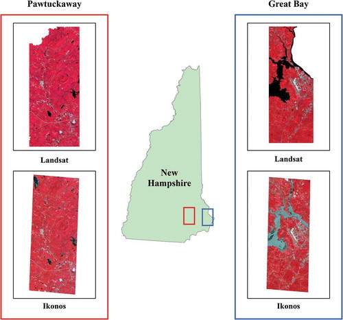
For the purpose of this study, two different areas in New Hampshire were selected: the Great Bay Watershed area and Pawtuckaway State Park; both located in the south eastern region of New Hampshire (Figure 1). Although these two areas are both in the same section of the state of New Hampshire, they represent diverse landscapes. Pawtuckaway State Park in Nottingham, NH contains approximately 2023.5 ha of land dedicated to recreation, and is comprised of forests, marshes, boulder fields, ledges, water bodies, and peatlands (nhdfl.org). Great Bay is an area closer to the seashore, and is comprised of forests, water bodies, and salt marshes. The region is representative of the intricate forest structure commonly found in the Northeast, yet also contains built up areas, clearings, wetlands, and open water. It is an area of great developmental expansion, as human population has grown in the region (Zankel et al. 2006).

Figure 1. Map depicting locations of study sites areas and imagery. For full colour versions of the figures in this paper, please see the online version.

Data

Two different types of imagery were utilized in this study. The first was Landsat 8 imagery collected on 25 August 2014. A single scene covered both study areas. The imagery was downloaded from EarthExplorer (http://earthexplorer.usgs.gov) and was georectified by the U.S Geological Survey prior to download In addition to the traditional, primary Landsat Thematic Mapper spectral bands (blue, green, red, near-infrared, and two shortwave infrared bands, 15-m panchromatic), Landsat 8 also collects an additional blue band for coastal and aerosol studies, a new shortwave infrared band for cloud detection, and two thermal bands (http://landsat.usgs.gov/ldcm_vs_previous.php). The thermal bands, panchromatic band, and cloud detection band were not included in this analysis, however. Most of the Landsat bands have a 30-m spatial resolution; however, the spatial resolution of the thermal bands is lower (100 m) while the panchromatic band has a higher resolution (15 m). For these reasons they were excluded. The cloud detection band was also excluded due to its placement well outside an atmospheric window in the electromagnetic spectrum. Most of the reflected energy from the ground within the region of the spectrum covered by this band would be absorbed by atmospheric moisture, and thus there would be very little information provided. The second set of imagery used in this study was Ikonos-2 collected on 15 September 2001. The scene was acquired from Spacing Imaging (now GeoEye). Two scenes, one for each study area, were required. The imagery was geometrically corrected prior to receiving it. The Ikonos scene contained 4 bands; blue, green, red, and near-infrared, all with a spatial resolution of 4 meters (Dial et al. 2003). The extent of the Landsat scene was significantly larger than that of the Ikonos, so the Landsat imagery was clipped to the extent of each of the Ikonos scenes. Since land cover classifications were not going to be performed, and all images were segmented independently, no further preprocessing was conducted.

Segmentation analysis

The multi-resolution segmentation algorithm was used to perform segmentation on the Landsat and Ikonos imagery. Multi-resolution segmentation is a bottom-up region-merging technique that starts by considering each pixel as a separate object, and then merges the objects based on user-specified homogeneity criteria. These object homogeneity is controlled with two parameters: (1) shape, which also controls color and (2) compactness which also controls smoothness. The shape criterion can have a value up to 0.9, and determines how much the shape of an image object influences the segmentation process compared to the objects spectral properties or color (Trimble 2014). The color parameter is based on the STDs of the spectral values associated with the initial pixel. The shape measure is controlled by weighting smoothness and compactness characteristics. The merging process terminates when the smallest increase of homogeneity exceeds the scale parameter threshold. Therefore, a higher scale parameter threshold will allow for more merging resulting in larger objects, and vice versa. While all parameters described play a role in the general shape and size of the resulting segments, the scale parameter has been found to have significantly greater control since it ultimately determines the overall amount of heterogeneity (Kim et al. 2011; Cánovas-García and Alonso-Sarría 2015). Several combinations of shape and compactness values were manually tested beforehand. Values of 0.2 and 0.5 (0.8 and 0.5 for color and smoothness, respectively) were chosen for the shape and compactness parameters, respectively. This combination applied greater weight to the spectral homogeneity of the objects which was important since unsupervised approaches utilize measures of spectral homogeneity. Compactness was set at 0.5 so as not to favor any particular shape. These values remained the same throughout the study; only the scale parameter was varied during the rest of the study.

A series of automated segmentations was produced at a range of scales. For the seven banded Landsat 8 imagery, the range was 20–200 in steps of 4 (20, 24, 28, 32, etc.), while the scale parameters for the four banded Ikonos imagery increased from 10 to 198 in steps of 4. Scale parameters of 198 and 200 resulted in significant under-segmentation for both sets of imagery, and thus were used as a maximum scale. During segmentation, all bands of each image were weighted equally. The mean and STD of the near-infrared band (NIR) band were then exported along with the final vectors for further analysis. The NIR band contains the greatest range of spectral values, and was found to be a good indicator of segmentation quality when using unsupervised evaluation methods (Kim, Madden, and Warner 2009; Johnson and Xie 2011). Thus, for efficiency, only the NIR band was used.

The exported scale parameters were then used to calculate local variance, Moran’s autocorrelation index, and the average weighted variance at each scale using ArcMap 10.2.2 (http://www.esri.com). Local variance was calculated by averaging the STD of all image objects at each segmentation scale. Global Moran’s I (MI) (Fotheringham, Brunsdon, and Charlton 2000) calculates the similarity between each object and its neighbors and then combines the results (Johnson et al. 2015). The equation for MI is shown below (Equation 1):

(1)

where:

w_ij is a measure of spatial adjacency of segment i and segment j,

y_i and y_j are the mean spectral values of the segment i segment j, and

is the mean spectral value for the whole image.

Low MI values indicate lower autocorrelation or higher between-object heterogeneity. The area-weighted variance ( was calculated as shown (Equation 2):

(2)

where:

a_i is the area of segment i and

v_i is the variance of segment i.

Lower weighted variance indicates higher within-object homogeneity. Before they could be utilized, MI values and had to be normalized so values were between 0 and 1 and could be compared. After normalization, the values were utilized to calculate the Global Score (GS) for each segmentation using the objective function below (equation 3):

(3)

where:

V_norm is the normalized weighted variance and

MI_norm is the normalized Moran I value.

Using the above formula, the optimal segmentation occurs at the highest GS score which indicates the point where between-object homogeneity is low (low MI) and within-object homogeneity is high (low wVar) (Johnson and Xie 2011; Espindola et al. 2006).

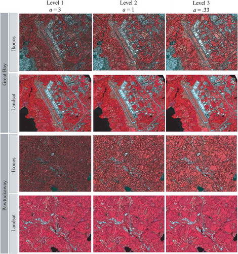
The segmentation F-measure proposed by Johnson et al. (2015) is given in Equation 4. MI_norm and V_norm are the same as those calculated above. a is the value that controls the weight of MI_norm and V_norm. GS_f was calculated for each scale in order to determine the best single-scale segmentation and three-level hierarchal segmentation parameters. A three-level hierarchal approach was suggested for landscape analysis (Drăguţ et al. 2014; Johnson et al. 2015). The three scale parameters were determined by calculating GS_f three times with a equal to 3, 1, and .33 for levels 1–3, respectively. These values (which are not scene dependent) were suggested by Johnson et al. (2015) to ensure the segmentation levels selected were different from each other in terms of the within- and between-object heterogeneity.

(4)

Results and discussion

A quantitative evaluation was performed to determine the optimal segmentation parameters using three measures: local variance, the objective function, and an F-measure. These measures were calculated for each image in each study area. For this evaluation, the shape and compactness parameters were kept at a constant value of 0.2 and 0.5, respectively. Scale parameters for the Landsat 8 and Ikonos imagery ranged between 20–200 and 10–198, respectively, with the scale value increasing by four with each run.

Local variance

Figure 2 shows the LV for each scale as well as the rate of change in LV (ROC-LV) from one scale to the next. The increase in variance is rapid at first but then levels off as the image objects become increasingly similar to one another with each merge. The optimal scale occurs when the LV at a certain scale (LV_n) is less than or equal to the LV at the previous scale (LV_n−1) (Drăguţ et al. 2014; Drǎguţ, Tiede, and Levick 2010). At no point was LV_n ≤ LV_n−1 for any of the imagery at either study area, meaning that the ROC-LV curve must be examined instead. Drǎguţ, Tiede, and Levick (2010) also consider the optimal scale as the first break in the ROC-LV curve after a continuous decay. On the graph, this would appear as a peak or step in the ROC-LV curve. For the Ikonos imagery, this first break occurs at scale 74 and 62 for Great Bay and Pawtuckaway, respectively (see Figure 2). For the Landsat imagery, the scale values were 68 and 60 for Great Bay and Pawtuckaway, respectively (see Figure 2).

Figure 2. Graph of local variance (LV) and rate of change in local variance (ROC-LV) for each scale separated by study area and imagery type. the axis for ROC-LV was rescaled to the first indication of optimal scale in order to make variations in the curve at courser scale easily visible. Note, Y axis scale for LV and ROC-LV differ between imagery types.

On the Ikonos imagery, the segments were large. Large homogenous objects such as large roof tops, open fields, parking lots were well segmented. Other features may be considered under-segmented due to the large scale parameters. For example, residential areas tend to be heterogeneous, small houses, trees, lawns, roads. At the scale chosen, all these features are merged into a singular object. Forest is a mixture of deciduous and coniferous species, and may even have breaks in the canopy exposing the ground. At these scales, predominately deciduous and coniferous stands are segmented, but smaller stands with a different composition are lost along with canopy openings, small wetlands, etc.

The Landsat imagery experiences similar difficulties. For smaller features in the landscape to be segmented, a small-scale parameter would be necessary. However, this approach did not indicate scales that were appropriate for these small features to be identified.

One of the benefits of this method for determining scale is that it is possible to determine multiple appropriate scales. With the ROC-LV curve this becomes difficult, as there are numerous peaks within the curve that could indicate a scale value to chose. The complexity of the scene being segmented can also increase the difficulty of scale selection. The ROC-LV curves of the Great Bay images, an area comprised of a mix of land covers, are much more variable than those of the Pawtuckaway study area curves. A relationship such as this was also noted in Drǎguţ, Tiede, and Levick (2010). In the case of this study, any additional appropriate scales chosen would be at scale parameters larger than the parameters stated above, meaning objects will continue to grow and incorporate more landscape features.

An appropriate scale for certain landscape features or cover types may never be indicated. As stated in Drǎguţ, Tiede, and Levick (2010), assuming there is a certain amount of spectral contrast between the object being delineated and the background, the object boundaries will be preserved across multiple higher scales. It is possible that the contrast between spectrally similar classes, like deciduous and mixed forest, would be too small to maintain the object boundaries long enough to impact the LV curve which could explain why finer scales, that would be necessary to distinguish small forest stands, were not indicated. The spatial resolution of the Landsat imagery, 30 meters, enhances this problem, as the spatial resolution blurs the transition from one feature to the next, reducing that contrast even more. Cánovas-García and Alonso-Sarría (2015) also noted that when spectral contrast between landscape features and their neighbors was low, a proper segmentation of these features was difficult regardless of what method was used to determine scale.

If the classes of interest are broad and spectrally different, for example forest vs. agriculture, then the automatic selection of scale parameters using this method could work reasonably well. However, with more complex classification schemes, automation may not be possible. The analyst will have to perform further investigation, increasing processing time. Additionally, it is believed that at each optimal scale, a particular feature within the imagery has been properly captured; however, because the process runs independent of the classes of interest, it is ultimately up to the analyst to decide what the scales chosen are delineating. For a wall-to-wall classification, this could lead to a substantial amount of investigation to determine the proper scale for various classes. Automated parameter selection using local variance may be better suited for feature extraction with high-resolution imagery. In this case, the analyst can choose the optimal scale that delineates a particular feature of interest such as trees or buildings where the boundary between one feature and the next is clear and distinct.

The objective function

Figure 3 shows the MI value for each scale parameter value tested for each scenario in this study. In all cases, as the scale parameter increased, the MI values continued to decrease meaning that as the objects became larger; they also became increasingly different spectrally from their neighboring objects. Kim, Madden, and Warner (2008) demonstrated how autocorrelation could be used to determine the optimal segmentation parameters. At small-scale parameter, a single homogenous area may be made of up multiple smaller segments, and as the scale parameter increases, these spectrally similar segments will merge and decrease the overall global autocorrelation values. After a certain scale parameter value is reached, the objects will begin to merge with objects representing different land cover types, once again increasing the autocorrelation. They determined that the lowest value was in fact the optimal scale parameter to use. Therefore, a V-shaped trend (decrease in MI followed by an increase) was expected. However, our study found that MI continuously decreased over the scale parameters investigated. Both Gao et al. (2011) and Johnson and Xie (2011) observed similar trends to those seen here using Landsat ETM+ data and high-resolution aerial imagery, respectively. Both studies were conducted in heterogeneous landscapes, much like this study, while Kim, Madden, and Warner (2008) study was conducted only within a forest, using IKONOS imagery. Given the trend in MI seen here, in a heterogeneous environment with multiple land cover types, the MI values will eventually exhibit the same trend that was seen in the Kim, Madden, and Warner (2008) study. However, that scale parameter to achieve this trend would occur well outside of the scale range investigated here. If and when that occurs, the objects would be significantly under-segmented. Autocorrelation alone may be better suited for class specific analysis rather than a global analysis as seen here.

Figure 3. Moran’s I values for each scale tested separated by study area and imagery type.

Figure 4 presents the GS for each scale determined using the objective function (Equation (3)) which combines both Moran’s I and weighted variance to determine the optimal scale parameter. Here, the optimal scale parameter is the one with the highest GS. All four graphs show a significant amount of variation in GS with scale. Both Landsat images had maximum GS values toward the higher end of the tested scale values; 180 and 152 for Great Bay and Pawtuckaway, respectively. For the Ikonos imagery, the maximum values were toward the low end of the tested scale parameters, 34 and 14 for Great Bay and Pawtuckaway, respectively.

Figure 4. Global score calculated using the objective function for each scale separated by study site and imagery type. higher values suggest better segmentations.

Figure 5 shows a subset of each study site segmented at the scale parameter determined by the objective function. For the Landsat imagery, the higher scale parameters resulted in very large segments. These scales were able to segment out large, spectrally homogeneous features on the landscape. Similar to the results of the LV method, broad land cover features were well distinguished such as forested areas, grassy or bare fields, water. Within forested areas, there was some distinction between larger, predominately deciduous versus coniferous stands. Smaller features such as vegetation embedded in development or vice versa were often not segmented, small tree stands embedded within a more homogenous forest matrix were also left out. Large heterogeneous residential areas were segmented, however small homogenous features within them were not. The Ikonos imagery was highly segmented using this approach. Smaller homogenous features (grassy lawns, small parking lots, small roof tops) were now well segmented, but larger homogenous features were over-segmented (Large roof tops, water, large open fields).

Figure 5. Each site and image segmented at their optimal single scale as determined by the objective function (Equation 3).

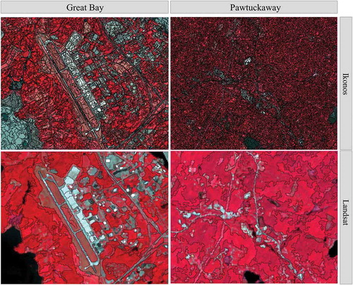
There is an interesting pattern to note here. Within each image type, the objective function suggested a higher scale parameter for the Pawtuckaway site. An indication such as this could be an indirect demonstration of the local approach proposed by Cánovas-García and Alonso-Sarría (2015). In their study, the authors utilized the objective function to identify an appropriate scale parameter to segment crops within a heterogeneous agricultural area. They found that by implementing a global approach to optimization (like done here), the objective function failed to pick an appropriate scale for some of the land cover types found in the diverse landscape they were working in. Instead when they segmented within a single agricultural field (localized approach), the objective function was better able to pinpoint a scale value that segmented the crops within that field. The key, they found, was spectral contrast. On a local scale, spectral contrast was larger between objects than on a global scale. The Pawtuckaway site was chosen because it was significantly less diverse than the Great Bay area, and comprised mostly of a single land cover type, forest. Segmentation within forested areas was very different between the two study sites. In the Great Bay areas, broader differences in forest reflectance were segmented (larger forest segments), compared to the Pawtuckaway area which segmented very fine differences. The Pawtuckaway site, in this case, may be acting as a localized approach to segmenting forest stands.

F-measure

Table 1 provides the single-scale and multi-scale values selected using the F-measure approach to selecting optimal scale parameters (Equation 4). It would appear that at a single-scale parameter, this formula was able to adjust for some of the problems noted with the values chosen by the objective function. The F-measure selected higher scale parameters for the Landsat imagery that seemed to have suffered from under-segmentation using the objective function. For the Ikonos imagery, the F-measure-chosen scale parameters were lower which adjusted for some of the over-segmentation.

Table 1. Optimal scale parameter values chosen for the single-scale and three-level multi-scale segmentations using the F-measure approach (Equation 4).

		Ikonos			Landsat
Site	Segmentation Type	Level 1	Level 2	Level 3	Level 1	Level 2	Level 3
Pawtuckaway	Single scale	38	-	-	84	-	-
	Three-level multi-scale	14	38	66	48	84	120
Great Bay	Single scale	34	-	-	64	-	-
	Three-level multi-scale	18	34	62	36	64	138

Despite the apparent improvement in scale parameters, under- and over- segmentation of features still remains a problem (Figure 6) because features on the landscape are best segmented at varying scales, not just one.

Several studies have found improved classifications when a multi-scale approach was implemented (Zhang et al. 2014; Drăguţ et al. 2014; Johnson and Xie 2013, 2011; Johnson et al. 2015). The F-measure equation contains an adjustable weight that controls the relative influences of the MI_norm and V_norm and thus the relative level of over- and under-segmentation. Examples of the three-level hierarchal segmentation for each image type and site are shown in Figure 7. The scale parameter selected is given in Table 1.

Figure 6. Each site and image segmented at their optimal single scale as determined by the F-measure approach (Equation 4).

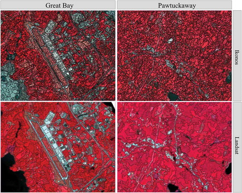
Figure 7. Optimal segmentations for the three-level hierarchical approach. The weighting parameter (a) used for each level is also given. Segmentation parameters are given in Table 1.

Higher weights allowed for finer scale parameters to be selected that will optimally segment small homogenous features. Smaller weights allowed for courser scale parameters to be selected that optimally segment larger homogenous features.

Conclusion

OBIA has become a popular tool for performing land cover classifications; however, the vital step of selecting the best segmentation scale parameters remains a difficult task. Empirical methods have been proposed with the goal of selecting an “optimal” set of scale parameters quickly and objectively compared to the commonly used trial and error approach. It is also assumed that selecting optimal scale parameters will result in the best accuracy. For these reasons, segmentation scale parameter optimization procedures are often implemented. The objective of this study was to test several unsupervised segmentation optimization procedures qualitatively and demonstrate that optimal parameters for a particular scene does not necessarily equate to optimal parameters for the chosen classification scheme. We tested several of these approaches with two different sets of imagery, moderate-resolution Landsat and high-resolution Ikonos, as well as in two study areas with different landscape characteristics.

The local variance approach was the least successful of those tested here, for both types of imagery at both study sites. Optimal scale parameters occur where LV_n ≤ LV_n−1 or when the LV at one scale is less than or equal to the LV of the previous scale. This criteria were not met for any of the scale parameters tested here leading to the use of the ROC-LV curve instead. Analysis of the ROC-LV curve is more time consuming and subjective as the user has to decide whether peaks in the curve suggest an optimal scale parameter and if so, what is being delineated and whether that is a feature of interest. Additionally, features of interest with low spectral contrast may not be indicated on this curve.

The objective function and F-measure approaches both work in a similar manner in that they use a combination of over- and under-segmentation measures to decide an optimal scale parameter. As a result of the way they are calculated, the user should always be able to compute a number. Both approaches worked reasonably well; however, there were some clear differences. Both approaches selected for finer scales in the Ikonos imagery and courser scales for the Landsat imagery. With the Ikonos imagery, this led to small features being well segmented but larger features were over-segmented. The problem was the opposite with Landsat imagery. When using the objective function, for both types of imagery, Pawtuckaway scales were much finer, most likely a result of the less diverse landscape within that image. The single-scale parameters selected by the F-measure approach seemed to correct for the over- and under-segmentation. Single-scale approaches; however, result in some locations being over-segmented and others being under-segmented. The adjustable weight on the F-measure approach allowed for multiple segmentation scale parameters to be determined to help alleviate this problem.

The key result and conclusion from this study is that there is currently no fool-proof method to determine optimal segmentation scale parameters for the purpose of feature extraction or land cover classification. Some limitations of these methods are described below.

1. Some methods may not provide meaningful results simply because of the image property it relies upon, for example the Local Variance method’s LV_n ≤ LV_n−1 rule.

2. Single-scale optimization approaches cannot ensure all the features of interest are segmented appropriately (e.g. The objective function or single-scale F-measure). As demonstrated, these methods help to select parameters that are optimal for the image in general which will vary based on the method used and the complexity of scene being segmented.

3. Optimization approaches that select for multiple scales can help to overcome the issues associated with only using a singular scale; however, the number of methods that accomplish this are far fewer and many require subjectively choosing or testing thresholds/weights. Johnson and Xie (2011) proposed the use of a heterogeneity index to refine over and under-segmentation, requiring the testing of several thresholds to decide what segments would be further refined since these values were unknown before-hand. The F-measure approach used here made use of weights which can control over and under-segmentation but the analyst must test values to find the number of levels and weights that best suit their purpose. This can reduce the objectivity of the segmentation process or increase processing time; two issues these optimization approaches are attempting to overcome.

Seeing as how these methods run independent of the features of interest, it is unrealistic to assume that these approaches will be able to select the best segmentation parameters for a wall-to-wall classification every time, even with a multi-scale approach demonstrated here. Supervised optimization approaches allow the analyst to incorporate information on the classes or features of interest into the process; however, they require the analyst to generate training data for all classes (Xun and Wang 2015; Yang, Li, and He 2014; Cheng et al. 2014) or already-existing GIS data (Guo and Du 2017) which might not always be available. With multiple classes, this can become time consuming.

Instead, these approaches can best be thought of as a way to narrow down parameter selection and save time, which has been suggested by others (Johnson et al. 2015; Belgiu and Drăguţ 2014; Cánovas-García and Alonso-Sarría 2015). Visual inspection will still be required to assess over- and under-segmentation or perform additional modifications. Räsänen et al. (2013) found the highest accuracy was achieved through visual inspection when compared to supervised methods, mentioning how, unlike the optimization methods used, they ultimately knew what they wanted from the segmentation.

Perhaps, determining the best or “optimal” scale based on image characteristics should not be the end goal when selecting segmentation scale parameters for classification. Belgiu and Drăguţ (2014) found classification accuracy was less dependent on the segmentation results. Instead they suggest as long as under-segmentation is kept to a minimum, high classification accuracies can still be achieved. For the purpose of performing a classification, the best segmentation should be considered the one that produces results with the highest accuracy. Campbell et al. (2015) used a multi-classification approaches to choose the best segmentations based on a particular classification scheme. While this would seem time consuming, the workflow can be semiautomated using programs such as R or eCognition (Trimble 2014) that allow have some programming capabilities and rule-set development (Cánovas-García and Alonso-Sarría 2015).

Acknowledgments

Partial funding was provided by the New Hampshire Agricultural Experiment Station. This is Scientific Contribution Number 2679. This work was supported by the USDA National Institute of Food and Agriculture McIntire Stennis Project #NH00077-M (Accession #1002519).

Disclosure statement

No potential conflict of interest was reported by the authors.

Additional information

Funding

Partial funding was provided by the New Hampshire Agricultural Experiment Station. This is Scientific Contribution number 2679. This work was supported by the USDA National Institute of Food and Agriculture McIntire Stennis Project number NH00077-M (Accession number 1002519).

References

- Baatz, M., and A. Schape. 2000. “Multiresolution Segmentation: An Optimization Approach for High Quality Multi-Scale Image Segmentation.” In Angewandte Geographische Informationsverarbeitung XII, edited by J. Strobl, T. Blaschke, and G. Griesebner, 12–23. Heidelberg: Wichmann-Verlag.
- Belgiu, M., and L. Drăguţ. 2014. “Comparing Supervised and Unsupervised Multiresolution Segmentation Approaches for Extracting Buildings from Very High Resolution Imagery.” ISPRS Journal of Photogrammetry and Remote Sensing 96: 67–75. doi:10.1016/j.isprsjprs.2014.07.002.
- Blaschke, T. 2010. “Object Based Image Analysis for Remote Sensing.” ISPRS Journal of Photogrammetry and Remote Sensing 65 (1): 2–16. doi:10.1016/j.isprsjprs.2009.06.004.
- Blaschke, T., C. Burnett, and A. Pekkarinen. 2004. “Image Segmentation Methods for Object-Based Analysis and Classification.” In Remote Sensing Image Analysis: Including the Spatial Domain, edited by S. M. De Jong and F. D. Van Der Meer, 211–236. Dordrecht, Netherlands: Kluver Academic Publishers. doi:10.1007/978-1-4020-2560-0.
- Campbell, M., R. G. Congalton, J. Hartter, and M. Ducey. 2015. “Optimal Land Cover Mapping and Change Analysis in Northeastern Oregon Using Landsat Imagery.” Photogrammetric Engineering & Remote Sensing 81 (1): 37–47. doi:10.14358/PERS.81.1.37.
- Cánovas-García, F., and F. Alonso-Sarría. 2015. “A Local Approach to Optimize the Scale Parameter in Multiresolution Segmentation for Multispectral Imagery.” Geocarto International 30 (8): 937–961. doi:10.1080/10106049.2015.1004131.
- Chabrier, S., B. Emile, C. Rosenberger, and H. Laurent. 2006. “Unsupervised Performance Evaluation of Image Segmentation.” EURASIP Journal on Advances in Signal Processing 2006: 1–12. doi:10.1155/ASP/2006/96306.
- Cheng, J., Y. Bo, Y. Zhu, and X. Ji. 2014. “A Novel Method for Assessing the Segmentation Quality of High-Spatial Resolution Remote-Sensing Images.” International Journal of Remote Sensing 35 (10): 3816–3839. doi:10.1080/01431161.2014.919678.
- Clinton, N., A. Holt, J. Scarborough, L. Yan, and P. Gong. 2010. “Accuracy Assessment Measures for Object-Based Image Segmentation Goodness.” Photogrammetric Engineering Remote Sensing 76 (3): 289–299. doi:10.14358/PERS.76.3.289.
- Conchedda, G., L. Durieux, and P. Mayaux. 2008. “An Object-Based Method for Mapping and Change Analysis in Mangrove Ecosystems.” ISPRS Journal of Photogrammetry and Remote Sensing 63 (5): 578–589. doi:10.1016/j.isprsjprs.2008.04.002.
- Dial, G., H. Bowen, F. Gerlach, J. Grodecki, and R. Oleszczuk. 2003. “IKONOS Satellite, Imagery, and Products.” Remote Sensing of Environment 88 (1–2): 23–36. doi:10.1016/j.rse.2003.08.014.
- Drăguţ, L., O. Csillik, C. Eisank, and D. Tiede. 2014. “Automated Parameterisation for Multi-Scale Image Segmentation on Multiple Layers.” ISPRS Journal of Photogrammetry and Remote Sensing 88: 119–127. doi:10.1016/j.isprsjprs.2013.11.018.
- Drǎguţ, L., D. Tiede, and S. R. Levick. 2010. “ESP: A Tool to Estimate Scale Parameter for Multiresolution Image Segmentation of Remotely Sensed Data.” International Journal of Geographical Information Science 24 (6): 859–871. doi:10.1080/13658810903174803.
- Duro, D. C., S. E. Franklin, and M. G. Dubé. 2012. “A Comparison of Pixel-Based and Object-Based Image Analysis with Selected Machine Learning Algorithms for the Classification of Agricultural Landscapes Using SPOT-5 HRG Imagery.” Remote Sensing of Environment 118: 259–272. doi:10.1016/j.rse.2011.11.020.
- Espindola, G. M., G. Camara, I. A. Reis, L. S. Bins, and A. M. Monteiro. 2006. “Parameter Selection for Region‐Growing Image Segmentation Algorithms Using Spatial Autocorrelation.” International Journal of Remote Sensing 27 (14): 3035–3040. doi:10.1080/01431160600617194.
- Ferguson, R. L., and K. Korfmacher. 1997. “Remote Sensing and GIS Analysis of Seagrass Meadows in North Carolina, USA.” Aquatic Botany 58 (3–4): 241–258. doi:10.1016/S0304-3770(97)00038-7.
- Flanders, D., M. Hall-Beyer, and J. Pereverzoff. 2003. “Preliminary Evaluation of Ecognition Object-Based Software for Cut Block Delineation and Feature Extraction.” Canadian Journal of Remote Sensing 29 (4): 441–452. doi:10.5589/m03-006.
- Fotheringham, A. S., C. Brunsdon, and M. E. Charlton. 2000. Quantitative Geography: Perspectives on Spatial Data Analysis. London: Sage. doi:10.1016/S0143-6228(97)90005-9.
- Gao, Y., J. Francois Mas, N. Kerle, and J. A. N. Pacheco. 2011. “Optimal Region Growing Segmentation and Its Effect on Classification Accuracy.” International Journal of Remote Sensing 32 (13): 3747–3763. doi:10.1080/01431161003777189.
- Guo, Z., and S. Du. 2017. “Mining Parameter Information for Building Extraction and Change Detection with Very High-Resolution Imagery and GIS Data.” Giscience & Remote Sensing 54 (1): 38–63. Taylor & Francis. doi:10.1080/15481603.2016.1250328.
- Jensen, J. R. 2016. Introductory Digital Image Processing: A Remote Sensing Perspective. 4th ed. Upper Saddle River, NJ: Pearson Prentice Hall.
- Johansen, K., L. A. Arroyo, S. Phinn, and C. Witte. 2010. “Comparison of Geo-Object Based and Pixel-Based Change Detection of Riparian Environments Using High Spatial Resolution Multi-Spectral Imagery.” Photogrammetric Engineering & Remote Sensing 76 (2): 123–136. doi:10.14358/PERS.76.2.123.
- Johnson, B., M. Bragais, I. Endo, D. M. Macandog, and P. Macandog. 2015. “Image Segmentation Parameter Optimization considering Within- and Between-Segment Heterogeneity at Multiple Scale Levels: Test Case for Mapping Residential Areas Using Landsat Imagery.” ISPRS International Journal of Geo-Information 4 (4): 2292–2305. doi:10.3390/ijgi4042292.
- Johnson, B., and Z. Xie. 2011. “Unsupervised Image Segmentation Evaluation and Refinement Using a Multi-Scale Approach.” ISPRS Journal of Photogrammetry and Remote Sensing 66 (4): 473–483. doi:10.1016/j.isprsjprs.2011.02.006.
- Johnson, B., and Z. Xie. 2013. “Classifying a High Resolution Image of an Urban Area Using Super-Object Information.” ISPRS Journal of Photogrammetry and Remote Sensing 83: 40–49. doi:10.1016/j.isprsjprs.2013.05.008.
- Kim, M., M. Madden, and T. Warner. 2008. “Estimation of Optimal Image Object Size for the Segmentation of Forest Stands with Multispectral IKONOS Imagery.” In Object-Based Image Analysis - Spatial Concepts for Knowledge-Driven Remote Sensing Applications, edited by T. Blaschke, S. Lang, and G. J. Hay, 291–307. Heidelberg, Germany: Springer. doi:10.1007/978-3-540-77058-9_16.
- Kim, M., M. Madden, and T. A. Warner. 2009. “Forest Type Mapping Using Object-Specific Texture Measures from Multispectral Ikonos Imagery : Segmentation Quality and Image Classification Issues.” Photogrammetric Engineering & Remote Sensing 75 (7): 819–829. doi:10.14358/PERS.75.7.819.
- Kim, M., T. A. Warner, M. Madden, and D. S. Atkinson. 2011. “Multi-Scale GEOBIA with Very High Spatial Resolution Digital Aerial Imagery: Scale, Texture and Image Objects.” International Journal of Remote Sensing 32 (10): 2825–2850. doi:10.1080/01431161003745608.
- Lathrop, R. G., P. Montesano, and S. Haag. 2006. “A Multi-Scale Segmentation Approach to Mapping Seagrass Habitats Using Airborne Digital Camera Imagery.” Photogrammetric Engineering & Remote Sensing 72 (6): 665–675. doi:10.14358/PERS.72.6.665.
- Lawrence, R. L., and A. Wright. 2001. “Rule-Based Classification Systems Using Classification and Regression Tree (CART) Analysis.” Photogrammetric Engineering and Remote Sensing 67 (10): 1137–1142.
- Liu, Y., L. Bian, Y. Meng, H. Wang, S. Zhang, Y. Yang, X. Shao, and B. Wang. 2012. “Discrepancy Measures for Selecting Optimal Combination of Parameter Values in Object-Based Image Analysis.” ISPRS Journal of Photogrammetry and Remote Sensing 68: 144–156. doi:10.1016/j.isprsjprs.2012.01.007.
- Möller, M., L. Lymburner, and M. Volk. 2007. “The Comparison Index: A Tool for Assessing the Accuracy of Image Segmentation.” International Journal of Applied Earth Observation and Geoinformation 9 (3): 311–321. doi:10.1016/j.jag.2006.10.002.
- Platt, R. V., and L. Rapoza. 2008. “An Evaluation of an Object-Oriented Paradigm for Land Use/Land Cover Classification.” The Professional Geographer 60 (1): 87–100. doi:10.1080/00330120701724152.
- Räsänen, Aleksi, Antti Rusanen, Markku Kuitunen, and Anssi Lensu. 2013. “What Makes Segmentation Good? A Case Study in Boreal Forest Habitat Mapping.” International Journal of Remote Sensing 34 (23): 8603–27. doi:10.1080/01431161.2013.845318
- Tong, H., T. Maxwell, Y. Zhang, and V. Dey. 2012. “A Supervised and Fuzzy-Based Approach to Determine Optimal Multi-Resolution Image Segmentation Parameters.” Photogrammetric Engineering & Remote Sensing 78 (10): 1029–1044. doi:10.14358/PERS.78.10.1029.
- Trimble. 2014. Ecognition Developer 9.0 User Guide. Munich, Germany: TrimbleGermany GmbH.
- Vogelmann, J. E., T. Sohl, and S. M. Howard. 1998. “Regional Characterization of Land Cover Using Multiple Sources of Data.” Photogrammetric Engineering & Remote Sensing 64 (1): 45–57.
- Whiteside, T. G., S. W. Maier, and G. S. Boggs. 2014. “Area-Based and Location-Based Validation of Classified Image Objects.” International Journal of Applied Earth Observation and Geoinformation 28 (May): 117–130. doi:10.1016/j.jag.2013.11.009.
- Witten, I. H., E. Frank, and M. A. Hall. 2011. Data Mining: Practical Machine Learning Tools and Techniques. 3rd ed. Burlington, MA: Morgan Kaufmann.
- Woodcock, C. E., and A. H. Strahler. 1987. “The Factor of Scale in Remote Sensing.” Remote Sensing of Environment 21 (3): 311–332. doi:10.1016/0034-4257(87)90015-0.
- Xun, L., and L. Wang. 2015. “An Object-Based SVM Method Incorporating Optimal Segmentation Scale Estimation Using Bhattacharyya Distance for Mapping Salt Cedar (Tamarisk Spp.) with Quickbird Imagery.” Giscience & Remote Sensing 52 (3): 257–273. Taylor & Francis. doi:10.1080/15481603.2015.1026049.
- Yang, J., P. Li, and Y. He. 2014. “A Multi-Band Approach to Unsupervised Scale Parameter Selection for Multi-Scale Image Segmentation.” ISPRS Journal of Photogrammetry and Remote Sensing 94: 13–24. doi:10.1016/j.isprsjprs.2014.04.008.
- Yu, Q., P. Gong, N. Clinton, G. Biging, M. Kelly, and D. Schirokauer. 2006. “Object-Based Detailed Vegetation Classification with Airborne High Spatial Resolution Remote Sensing Imagery.” Photogrammetric Engineering & Remote Sensing 72 (7): 799–811. doi:10.14358/PERS.72.7.799.
- Zhang, H., J. E. Fritts, and S. A. Goldman. 2008. “Image Segmentation Evaluation: A Survey of Unsupervised Methods.” Computer Vision and Image Understanding 110: 260–280. doi:10.1016/j.cviu.2007.08.003.
- Zhang, L., K. Jia, X. Li, Q. Yuan, and X. Zhao. 2014. “Multi-Scale Segmentation Approach for Object-Based Land-Cover Classification Using High-Resolution Imagery.” Remote Sensing Letters 5 (1): 73–82. doi:10.1080/2150704X.2013.875235.
- Zhang, X., X. Feng, P. Xiao, G. He, and L. Zhu. 2015. “Segmentation Quality Evaluation Using Region-Based Precision and Recall Measures for Remote Sensing Images.” ISPRS Journal of Photogrammetry and Remote Sensing 102: 73–84. doi:10.1016/j.isprsjprs.2015.01.009.
- Zhang, X., P. Xiao, and X. Feng. 2012. “An Unsupervised Evaluation Method for Remotely Sensed Imagery Segmentation.” IEEE Geoscience and Remote Sensing Letters 9 (2): 156–160. doi:10.1109/LGRS.2011.2163056.