Mapping drought-impacted vegetation stress in California using remote sensing

Abstract

Recent droughts and the profound effects they have on ecosystems, agriculture, and forests in California highlighted a critical need to understand drought impacts and develop remote sensing-based methods for drought monitoring. The objectives of this work were to evaluate drought-affected areas of northern and central California using remote sensing and aid in drought mitigation and prediction efforts for sustainable forest resource management and planning. Remote sensing provides direct measurement of spectral properties at moderate spatial resolution (30 m with Landsat) as compared to modeled environmental variables at 800 m spatial resolution, scaled to 270 m. Modified Perpendicular Drought Index derived from Landsat data and long term Climatic Water Deficit (CWD) data for the year 2014 were analyzed. MPDI was strongly correlated with CWD, precipitation and temperature data for various forest types with coefficient of determination in the range of 0.60–0.80. Our results demonstrate that MPDI is an effective and direct method to monitor vegetation stress and forest declines at landscape scale, thereby providing land managers and stakeholders guidance in forest management and planning.

Keywords:

• California Drought
• Mapping
• Landsat 8 OLI
• Drought Index

View correction statement:

Corrigendum

1. Introduction

The recent drought in California seriously affected not just the agricultural sector, but also the natural resources sector including forestry, wildlife, and fisheries. Some of the ecological implications that are predicted to worsen include water conservation, forest health (pest and disease), fire risk and severity, and other societal implications such as farm labor, livestock, and food prices (Howitt et al. 2014). California experienced the warmest January to June with a temperature of 2.67°C above average and 0.61°C warmer than the previous record (NOAA 2014). As of July 15, 2014, the National Weather Service drought monitor shows 81% of California in the category of extreme drought. While the State Water Resources Control Board has suspended its water conservation regulation due to relatively wet winter and spring during 2016, three-quarters of the state continued to experience moderate to severe drought (http://pacinst.org/).

Although drought is a complex natural phenomenon, it can be described and monitored by a simplified drought index, which is a single quantitative number assimilating a large amount of environmental data. The index allows scientists to quantify climate anomalies in terms of intensity, duration, and spatial extent, making it easier to communicate the information to diverse users (Wilhite et al. 2000). In the United States, great efforts have been made to develop a variety of drought indices (Heim, 2000); the most widely used are the Palmer Drought Severity Index (PDSI) (Palmer, 1965), the Crop Moisture Index (Palmer, 1968), the Surface Water Supply Index (Shafer and Dezman, 1982), and the Standardized Precipitation Index (SPI) (McKee et al., 1993 and McKee et al., 1995). About 150 drought indices have been proposed to characterize drought at regional to national levels (Zargar et al. 2011; Niemeyer 2008). All of these indices are continuous functions of one or more hydro-meteorological variables such as precipitation, temperature, soil water, streamflow, groundwater, potential evapotranspiration, etc. (WMO, 1975). Owing to this variation, most of the drought indices are developed for specific regions, and thus have inherent limitations under different climatic conditions.

In the last three decades, remote sensing has provided a useful tool for drought monitoring and a variety of remotely sensed drought indices based on vegetation indices, land surface temperature (LST), albedo, etc. have emerged. Several drought indices have been proposed based on normalized different vegetation index (NDVI, Rouse et al. 1974) to monitor drought severity such as the Anomaly Vegetation Index (AVI) and the Vegetation Condition Index (VCI) (Chen, Xiao, and Sheng 1994; Kogan 1995a), Modified Perpendicular Drought Index (MPDI) (Ghulam et al. 2007b), Temperature Drought Vegetation Index (TDVI) (Sandholt et al. 2002) and Vegetation Temperature Condition index (VTCI) (Wang et al. 2001; Ceccato et al. 2002).

Drought is a complex issue dependent upon evapotranspiration, temperature, rainfall, available soil moisture content and groundwater. Similar to other methods developed to estimate surface biophysical variables, remote sensing of drought is at the core of a common problem in algorithm development – the inability to generalize across studies spread over different geographic regions. Numerous case studies applied to varying climatic test sites are essential to generalize such new developments in both space and time.

A direct and simple method for the estimation of surface dryness, namely the perpendicular drought index (PDI), has been developed (Ghulam, Qin, and Zhan 2007a) and found to be effective in large-area applications over western China using Moderate Resolution Imaging Spectroradiometer (MODIS) data (Qin et al. 2008 and Rungsipanich and Chansury, 2008). In order to account for soil and vegetation cover heterogeneity, Ghulam et al. (2007b) modified the perpendicular drought index. The modified perpendicular drought index (MPDI) is a combination of two important indicators of drought – soil moisture (SM) and fraction of green vegetation (fv). The method shows potential advantages for regional surface dryness estimation (Ebrahimi et al. 2010; Shahabfar and Eitzinger 2011). In addition to the NDVI, the MPDI was selected for this data analysis. The literature indicates robustness of MPDI in estimating drought conditions with sensitivity to plant cover dynamics (Ghulam et al. 2007b; Shahabfar, Ghulam, and Eitzinger 2012; Qin et al. 2008).

The main objective of this paper was to map vegetation stress in the drought-affected areas of northern and central California using the MPDI with the overall intent to aid drought monitoring, mitigation and prediction efforts in California. We were especially interested in the relationship between MPDI (a remote sensing based approach) and Climate Water Deficit (an environmental modeling approach) to drought evaluation. If correlated, the remote sensing data could provide a direct measurement of spectral properties of the landscape at finer spatial resolution (30 m) than the modeled approach (800 m modeled to 270 m). Additionally, the approach could be easily applied to other newer sensor data such as the Sentinel – 2 that collect NIR-Red reflectance data.

2. Study area and data

Figure 1 shows the spatial extent of the study area in the state of California. The study area provides a representative sampling of important forested environments of the state along the Sierra Nevada range that extends more than 400-kms northward from the Mojave Desert to the Cascade Range of northern California (britanica.com/place/Sierra-Nevada-mountains). Out of the twelve national forests that span the state, the study area intersects nine of them, and the some of the major ones include the Lassen and Plumas National Forests in the North, Tahoe, and Eldorado in the central region, and Stainslaus and Sierra, and a small portion of Sequoia National Forests in the South. The elevation ranges from 500 to 2000 m above mean sea level as shown in Figure 1.

Figure 1. Map of the study area in California. The yellow polygon represents the spatial extent of the study, while the hashed boxes represent the footprint of the Landsat 8 OLI imagery. The green polygons represent the boundary of the national forests in the region. The lower inset shows the elevation contours (blue:500 m; yellow:1500 m; and red:2000 m). For full colour versions of the figures in this paper, please see the online version.

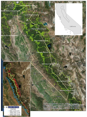
The mid-latitude location of the Sierras and its proximity to the moderating influence of the Pacific Ocean give the Sierra Nevada an unusually mild mountain climate, with precipitation averaging from about 760 mm in the western foothill zone to 1900 mm in the northern half of the range. The wind pattern over the Sierras, called the Pacific High anticyclone, is strong during the summer resulting in a seaward draw of dry air across the mountains. This high-pressure zone often during successive winters results in mid-latitude jet stream that is weak or pushed to the north. Most often this phenomenon results in drought as evidenced during the mid-1930s, mid-1970s, and mid-1980s to early 1990s.

The vegetation communities in the study area are distinguished based on slope and elevation gradients across the range. The lower foothills support mostly deciduous trees and shrubs, as well as the evergreen interior live oak. Black oak, Ponderosa pine, and incense cedar occur in the upper foothills. The montane forest, which constitutes the primary commercial timber zone, contains Douglas fir, red fir, Jeffrey pine, and the celebrated big tree, or giant sequoia, for which Sequoia National Park was designated a public preserve. Lodgepole pine, mountain hemlock, Sierra juniper, and western white pine are among the trees of the subalpine forest. Mosses, lichens, and low-flowering Alpine plants prevail above the tree line. The arid eastern slopes support sagebrush, bitterbrush, juniper, piñon pine, and aspen. Chaparral, a shrub-like assemblage of broad-leaved evergreen shrubs dominated by chamise, scrub oak, manzanita, and caeonothus, grows in all but the Alpine zones on both sides of the range.

A multisource geospatial database consisting of Landsat imagery and GIS data was assembled for analysis. Cloud-free Landsat-8 OLI (Operational Land Imager) imagery for the June-August 2014 time was downloaded from the USGS Earth Explorer website (http://earthexplorer.usgs.gov/). Specifically, seven Landsat image tiles (42p/35r, 27-Aug; 43p/33r, 18-Aug; 43p/34r, 01-July; 44p/31r, 24-Jul; 44p/33r, 24-Jul; 44p/32r, 24-Jul; and 42p/34r, 08-Jun) for the summer period (June-August) of 2014 were included in the analysis. Elevation data at 30-m spatial resolution was acquired from USGS National Elevation Dataset (USGS-NED, nationalmap.gov), while environmental data pertaining to long-term climate data (1981–2010) was downloaded from PRISM site maintained by the Oregon State University (prism.oregonstate.edu). Additionally, climatic Water Deficit (CWD) was collected from the USGS California Water Science Center (https://ca.water.usgs.gov/), and Landfire data from the USFS (landfire.gov).

Eight scenes (Dates: footprints shown in Figure 1) for the summer period of 2014 (May-June) that encompass the study area were downloaded. After stacking the individual data bands into a composite image, major preprocessing analysis of the satellite images involved radiometric correction and reprojection to the Albers USGS (CA) Teal coordinate system. The ATCOR3 module within ERDAS Imagine software was used to radiometrically correct the imagery using a 30-m USGS DEM to account to elevation variations. Other preprocessing analysis of the data involved clipping the image stack to the boundary of the study area and reprojecting to the NAD83 California Teale Albers coordinate system.

3. Methods

3.1. Modified perpendicular drought index (MPDI)

Numerous studies have documented the application of MPDI (Chen, Li, and Zhang 2015; Ghulam et al., 2007b; Li and Tan 2013). MPDI, as the name suggests is a modification of the PDI or the Perpendicular Drought Index (Figure 2), and it is the straight-line distance from the Vegetation Index line (PVI) and the Soil line BCD. If pixel values from the NIR and Red bands specific to bare soil area can be plotted, the pixel values would orient along the soil line (BCD), such that pixels representing higher moisture content would lie closer to the origin and those pixels that are having lower moisture content would be further from the origin. The pixels when having varying vegetation cover would orient more towards the NIR region as shown by the shaded area in Figure 2. These two distribution are represented by orthogonal lines and combined in the MPDI function. Additional details about the algorithm are available from Ghulam (2007b). The slope (M) of the soil line is an important parameter used in the MPDI algorithm along with the NDVI-based power function for vegetation fractional cover.

Figure 2. Important linear relationship of soil line and the vegetation response in the NIR-Red feature space used in the MPDI algorithm (Source: Ghulam et al., 2007a).

The MPDI expression is

where is defined as the fraction of ground surface covered by vegetation (Baret, Clevers, and Steven 1995). and are the pure vegetation reflectances in the Red and NIR bands, respectively. When other variables, such as leaf water content, leaf angle distribution, sun, and viewing geometry, are fixed, variations in canopy reflectance are dependent on that causes variations in canopy reflectance. (i.e., it is , not and Rv, NIR, that causes the canopy reflectance variations). In this study, and have estimated values of 0.05 and 0.5, respectively (Ghulam et al. 2007b). In addition to Red and NIR reflectance, the MPDI is dependent not only on soil moisture status but also on vegetative growth governed by activity rates, greenness, and stress levels.

A power function transforms the scaled NDVI (Jiang et al. 2006; Baret, Clevers, and Steven 1995; Matkan et al. 2010) to calculate vegetation fraction using:

where corresponds to vegetated surface with maximum NDVI and infinite leaf area index ( = 1), while corresponds to bare soil surface ( = 0). In this study, the vegetation fraction was calculated by visually querying for the maximum and minimum NDVI values.

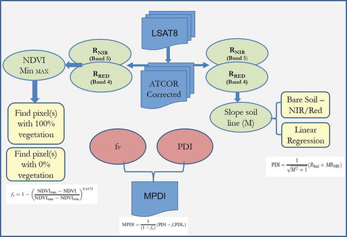
Figure 3 shows the workflow implemented for processing the radiometrically correct imagery. The workflow represents the image processing steps undertaken to implement the MPDI spectral index using parameters derived from the Landsat spectral band data, particularly the slope of the soil line and the vegetation fractional components.

Figure 3. Workflow routine for implementation of the Modified Perpendicular Drought Index.

3.2. Soil line derivation

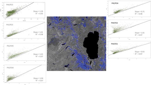
The soil line was derived based on the Red-NIR reflectance from sampled areas that represent bare soils. To focus on the bare soil areas, a unique approach was adopted. An unsupervised classification of the atmospherically corrected satellite image data was performed. The resulting 25 clusters of pixels were visually analyzed to identify the bare soil class. In general, clusters 19–25 were representative of the bare soil areas (see Figure 4). The pixels within these bare areas were sampled using a Latin Hypercube sampling method (Minasny and McBratney 2006). Basically, the sampling process adopts a stratification approach that constrains sampling based on ancillary information that included Red and NIR reflectance, location coordinates, and land cover information. The sampling process resulted in 2000 samples that were used to derive the soil line using a binning process implemented in R, to produce representative values within the grouping intervals of the large sampling reflectance data. The approach focused on deriving the soil regression line based on the mean of the bottom 1% of the pixel values in each bin. A sample of the regression modeling of the soil line is shown in Figure 4. Parameters pertaining to the MPDI algorithm such as Slope and Intercept were derived from the regression line.

Figure 4. Bare areas classification output (blue patches) that was used to derive the soil line for an example image tile (Lake Tahoe region). The plots show soil line plots extracted based on sampling the bare areas in each of the Landsat image tiles covering the study area.

3.3. Modified perpendicular drought index analysis

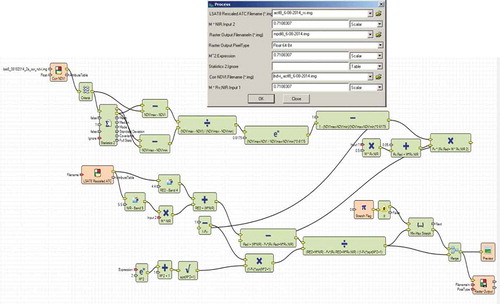
A spatial model (Figure 5) was developed in ERDAS Imagine (http://www.hexagongeospatial.com/) to implement the drought algorithm and batch process the Landsat image tiles for the study area. The model basically takes the atmospherically corrected Landsat image data file and the slope parameter as input and parses out the spectral bands relevant for the MPDI calculation. The user specifies the location of the image file along with the slope parameter extracted from the slope line derived for the same image file. The functions built within the spatial model extracts the bands specific for the vegetation fraction calculation and shunts the output to the MPDI algorithm function. The output is a raster image file where each pixel represents the MPDI value from a 0–1 scale.

Figure 5. Spatial model illustrating the calculation of the MPDI algorithm using the Landsat spectral bands and the soil parameter. The top chain of the model calculates the vegetation fraction and shunts it to the lower chain where the MPDI is calculated to output a raster grid.

3.4. Correlation analysis of MPDI to environmental data

In the absence of field level soil moisture data, the Climatic Water Deficit (CWD) data were acquired from the USGS Water Science Center, as mean monthly summary raster files for the summer months. The CWD and its related changes serve as a good surrogate for the soil moisture status since it represents the difference between the Potential ET and the Actual ET (Stephenson 1998, Cornwell et al. 2012). CWD effectively integrates the combined effects of solar radiation, evapotranspiration, and air temperature over watershed conditions given available soil moisture derived from precipitation. And so, CWD provides another interpretation of additional amount of water that would have evaporated or transpired had it been present in the soils given the temperature forcing. The CWD data sets are available as mean monthly values of water deficit represented as raster GIS layers. The raster GIS layers for the April–May period were averaged to produce a single raster output. Additionally, anomaly analysis of the 2014 CWD was conducted by comparing it to the mean CWD of the past 30 years of CWD. This map calculation involves:

CWD_Anom = MeanCWD₃₀  –  MeanCWD_2014 s

where, CWD_Anom refers to the Anomaly in CWD; MeanCWD₃₀ indicates 30 year mean CWD; and CWD_2014 s refers to the summer mean CWD for the 2014 year.

Land cover representing the different forest types for the study area was produced using a combination of analysis that included an unsupervised classification of the Landsat imagery and refining the output clusters using the USFS Landfire data.

30-year (1981–2010) normal of climate data for the summer months (May-August) acquired from PRISM (Precipitation-elevation Regressions on Independent Slopes Model, Daly et. al 1994) were processed to generate raster GIS layers for min temperature, maximum temperature, mean temperature, relative humidity, wind speed, and precipitation. The historical record was processed to extract the cell median for the summer months (May, June, July, August) specific to the study area region.

Additionally, using the forest classes as zones, the MPDI values were extracted using Zonal Statistics function within GIS. The extracted MPDI values for each of the zones were appended back to the forest class layer using join operation. Similarly, the CWD and the climate GIS data were extracted and appended to the forest layer to create a consolidated data table. This table was exported to a spreadsheet to further process and visualize the data as simple scatter plots with trend lines.

4. Results and discussion

The spatial distribution of MPDI calculated using the spatial model and acreage plots are shown in Figure 6. MPDI values between 0.15 and 0.35 are indicative of vegetation stress most likely associate with moisture stress. These thresholds were based on user interpretation of the outputs using 1-m 2014 NAIP (National Agricultural Imagery Program) data, and are also within the range (0.2–0.4) observed for ≤20% soil moisture that is usually associated with vegetation wilting and drought conditions (Ghulam et al., 2007). These areas are highlighted in orange-red colors on the map shown, green areas are non-stressed and tan areas are beginning to show stress. The higher values of the MPDI values above 0.4 are mostly associated with extremely arid areas of the landscape that are soil, rock, or dead annual vegetation.

Figure 6. Vegetation stress mapped using the MPDI along with the percent area covered (insert chart) for the study area.

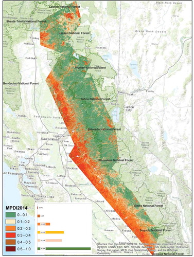
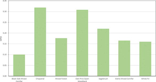
About 32.61% of the study area represents high impacts of drought based on the MPDI data, with about 20.32% of the area beginning to show vegetation stress. The spatial distribution of the vegetation stressed areas was evaluated using the classified forest types map produced derived by evaluating 51 clusters of spectral classes cross-walked with the Landfire forest types (Figure 7). Based on the zonal statistics of the MPDI values within the different forest types mapped, Oak-pine woodland, mixed forest, Sierra mixed Conifer, along with Chaparral and Sagebrush were some of the major forest types associated with the sensitive MPDI range (MPDI 0.15–0.35) of vegetation stress (Figure 8). Oak-Pine Open Woodland consisting mostly of Blue Oak along with Chaparral forest types showed high response (0.32 and 0.31 respectively), while Sagebrush and mixed forest (mostly Ponderosa and Jeffrey pine) showed relatively lower response of 0.22 and 0.18, respectively. Similar responses were observed for Sierra Mixed Conifer and White Fir forest types with 0.17 and 0.16 MPDI values, respectively, while Black Oak-Mixed Conifers showed an MPDI response of 0.10.

Figure 7. Forest types mapped using 2014 summer Landsat8 data.

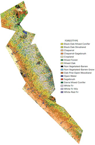
Figure 8. The distribution of MPDI values for the mapped forest types in the study area.

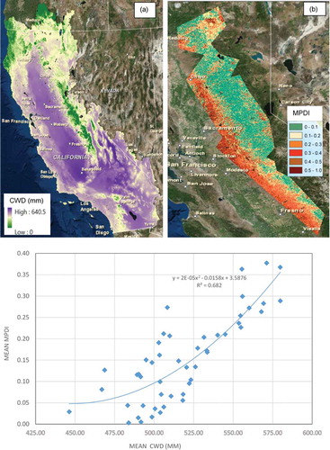
Additional analysis and validation of the MPDI output involved comparison to the environmental data, particularly the Climatic Water Deficit (CWD) data (Figure 9). The mean MPDI values for the forest classes (51 clusters) were extracted using Zonal Stats GIS function and compared to the corresponding mean CWD for the same zones. The comparison was evaluated using a scatter plot that showed a significantly high correlation (R² = 0.68).

Figure 9. Regression analysis fitting the Mean CWD (a) to the Mean MPDI (b) for the different forest types in the study area.

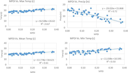
Anomaly analysis of the CWD for 2014 when compared to the past 30-year mean CWD is shown in Figure 10. Based on a deviation range of 0 to −420 mm from historical 30-year summer mean, forested areas within the study area showed high deviation. Similarly, analysis of the MPDI relationship to climate variables extracted from the PRISM database showed strong relationship as shown in (Figure 11).

Figure 10. Distribution of the CWD anomaly of summer 2014 data from historical 30-year summer mean.

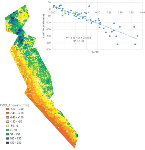
Figure 11. MPDI relationship to weather variables.

5. Conclusions

This study highlights an effective method for drought monitoring and assessment using the modified perpendicular drought index (MPDI) based on near-infrared and red reflectance data, readily available from Landsat 8 imagery. The general connotation of drought implying drier-than-normal conditions that result in water-related problems is mostly interpreted from an agro-meteorology context, depending on how water deficiency affects the system. There is the agricultural drought, signifying lack of soil moisture; meteorological drought, denoting a lack of observed precipitation; and hydrological drought, signifying reduced streamflow/groundwater levels.

While numerous studies have highlighted the use and application of drought indices mostly for agricultural and grassland ecosystems, little literature exists for specific applications within forested systems. There could be numerous reasons for this including the fact that forested systems are natural occurring landscape features with very high variability in terms of forest types, terrain and environmental conditions that provide a diverse canopy structure and conditions leading to challenges in implementing a spectral index. Owing to the robustness of the MPDI spectral index, the results of the analysis presented in this study demonstrate a unique capability and potential for drought monitoring in forested ecosystems of California. Additionally, the relevance of such remote sensing-based characterization of vegetation stress within forest communities is crucial due to California’s megadrought conditions, the impacts of which will exist for many years to come. When compared to hydrological models that use simulated/interpolated weather data and implement process/state modeling approach, the importance of using a satellite data-based spectral index such as the MPDI, clearly demonstrates the objectivity and usefulness of innovative applications of satellite data and algorithm for vegetation stress assessment in forest ecosystems, particularly at high spatial (30-m) and temporal resolutions (16-day), thereby providing land managers and stakeholders an operational framework for planning and management.

The MDPI study presented here was validated using climate water deficit (CWD) data. Our analysis revealed that MPDI was strongly correlated with CWD, precipitation and temperature data for various forest types with coefficients of determination in the range of 0.60–0.80. The CWD calculated as the amount of water by which potential evapotranspiration (PET) exceeds actual evapotranspiration, provides an effective proxy for quantifying drought stress, as the deficit index integrates the sum effects of solar radiation, evapotranspiration, and air temperatures under available soil moisture conditions derived from precipitation (Stephenson 1998, Cornwell et al. 2012, Flint and Flint 2012). An important outcome of our analysis provides a more robust and rapid assessment of vegetation stress and impacts due to drought conditions using the robust MPDI index.

Furthermore, MPDI analysis conducted in this study related to forested ecosystems, which contrasts with previous studies that focused predominantly on agricultural and grassland ecosystems. MPDI thresholds of 0.15–0.35 were identified as uniquely corresponding to vegetation stress zones in the forested cover types of the study region. Thus, our study provides valuable contribution to the knowledgebase of using remote sensing based spectral indices such as the MPDI to distinguish and map vegetation stress and drought severity for forested ecosystems.

One major limitation of MPDI identified in this study relates to the vegetation fraction component of the MPDI algorithm. While the main intent of using the power function of the scaled NDVI is to reduce effects of atmospheric perturbations, additional sensitivity analysis involving the NDVI_min and NDVI_max and related power term needs to be further investigated. Additionally, while sensitivity of the index to using other spectral bands has been demonstrated with respect to canopy water content (Ceccato et al. 2002; Zarco-Tejada, Rueda, and Ustin 2003) efforts are underway to understand the implications of thermal and SWIR wavelength bands within the MPDI algorithm.

Overall, MPDI characterizes vegetation cover types and moisture dynamics through a simple and effective model that integrates data from readily available NIR-Red spectral data. Ongoing efforts to understand drought conditions and related vegetation stress using MPDI in a spatio-temporal framework involving historical Landsat data are in progress to further demonstrate the robustness and applicability of the index.

Acknowledgments

This work was supported by a research grant funded by the Pacific Gas and Electric (PG&E) - Vegetation Management Program (2014/2015). The authors thank Drs. Lorraine Flint and Alan Flint (USGS California Water Science Center) for providing the climate water data and for valuable input in the data analysis. Also, special thanks to Melissa Kimble for help in preprocessing the Landsat data.

Disclosure statement

No potential conflict of interest was reported by the authors.

Additional information

Funding

This work was supported by a research grant funded by the Pacific Gas and Electric (PG&E) - Vegetation Management Program (2014/2015).

References

- Baret, F., J. G. P. W. Clevers, and M. D. Steven. 1995. “The Robustness of Canopy Gap Fraction Estimations from Red and Near-Infrared Reflectances: A Comparison of Approaches.” Remote Sensing Environment 54 (2): 14–151. doi:10.1016/0034-4257(95)00136-O.
- Ceccato, P., N. Gobron, S. Flasse, B. Pinty, and S. Tarantola. 2002. “Designing a Spectral Index to Estimate Vegetation Water Content from Remote Sensing Data: Part 1 Theoretical Approach.” Remote Sensing of Environment 82 (2–3): 188–197. doi:10.1016/S0034-4257(02)00037-8.
- Chen, N., J. Li, and X. Zhang. 2015. “Quantitative Evaluation of Observation Capability of GF-1 Wide Field of View Sensors for Soil Moisture Inversion.” Journal Applications Remote Sens 9 (1): 097097. 0001. doi:10.1117/1.JRS.9.097097.
- Chen, W., Q. Xiao, and Y. Sheng. 1994. “Application of the Anomaly Vegetation Index to Monitoring Heavy Drought in 1992.” Remote Sensing of Environment 9 (2): 106–112.
- Cornwell, W.K, S Stuart, A Ramirez, C.R Dolanc, J.H Thorne, and D.D. Ackerly 2012. "Climate Change Impacts On California Vegetation: Physiology,life History, and Ecosystem Change. California Energy Commission. Publication number: CEC-500-2012-023. Available from: http://www.energy.ca.gov/2012publications/CEC-500-2012-023/CEC-500-2012-023.pdf.
- Daly, C., R. P. Neilson, and D. L. Phillips. 1994. “A Statistical-Topographic Model for Mapping Climatological Precipitation over Mountainous Terrain.” Journal of Applied Meteorology 33: 140–158. doi:10.1175/1520-0450(1994)033<0140:ASTMFM>2.0.CO;2.
- Ebrahimi, M., A.A. Matkan, and R. Darvishzadeh, 2010. Remote sensing for drought assessment in arid regions (a case study of central part of Iran, Shirkooh Yazd).In: Wagner, W., Székely, B. (Eds.), ISPRS TC VII Symposium – 100 Years ISPRS. Vienna, Austria, July 5–7, 2010. Vol. XXXVIII, Part 7B, pp. 199–203.
- Flint, L. E., and A. L. Flint. 2012. “Downscaling Future Climate Scenarios to Fine Scales for Hydrologic and Ecological Modeling and Analysis.” Ecological Processes 1:2. doi:10.1186/2192-1709-1-2.
- Ghulam, A., Q. Qin, T. Teyip, and Z. L. Li. 2007b. “Modified Perpendicular Drought Index: A Real Time Drought Monitoring Method.” ISPRS Journal Photogramm 62 (2): 150–164. doi:10.1016/j.isprsjprs.2007.03.002.
- Ghulam, A., Q. Qin, and Z. Zhan. 2007a. “Designing of the Perpendicular Drought Index.” Environment Geological 52 (6): 1045–1052. doi:10.1007/s00254-006-0544-2.
- Heim, R. R. 2000. "Drought Indices: A Review", in Drought: A Global Assessment, Hazards Disasters Ser., vol. I, edited by D. A. Wilhite, 159–167. Routledge, New York.
- Howitt, R., J. Medellin-Azuara, D. MacEwan, J. Lund, and D. Summer. 2014. Economic Analysis of the 2014 Drought for California Agriculture. https://watershed.ucdavis.edu/files/content/news/Economic_Impact_of_the_2014_California_Water_ Drought.pdf
- Jiang, Z., A. Huete, J. Chen, Y. Chen, J. Li, G. Yan, and X. Zhang. 2006. “Analysis of NDVI and Scaled Difference Vegetation Index Retrievals of Vegetation Fraction.” Remote Sensing Environment 101 (3): 366–378. doi:10.1016/j.rse.2006.01.003.
- Kogan, F. N. 1995. “Droughts of the Late 1980s in the United States as Derived from NOAA Polar-Orbiting Satellite Data.” Bulletin of the American Meteorological Society 76 (5): 655–668. doi:10.1175/1520-0477(1995)076<0655:DOTLIT>2.0.CO;2.
- Li, Z., and D. Tan. 2013. “The Second Modified Perpendicular Drought Index (MPDI1): A Combined Drought Monitoring Method with Soil Moisture and Vegetation Index.” Journal of the Indian Society of Remote Sensing 41 (4): 873–881. doi:10.1007/s12524-013-0264-5.
- Matkan, A. A., R. Darvishzadeh, A. Hosseiniasl, and M. Ebrahimi. 2010. “Estimation of Vegetation Fraction in Arid Areas Using ALOS Imagery.” Proceedings SPIE 7824: (78242E). doi:10.1117/12.864826.
- McKee, T. B., N. J. Doesken, and J. Kleist. 1993. "The Relationship of Drought Frequency and Duration of Time Scales". Eighth Conference on Applied Climatology, American Meteorological Society, Jan17-23, 1993, Anaheim CA, pp.179–186.
- McKee, T. B., N. J. Doesken, and J. Kleist, 1995. "Drought Monitoring With Multiple Time Scales". Ninth Conference on Applied Climatology, American Meteorological Society, Jan15-20, 1995, Dallas TX, pp.233–236
- Minasny, B., and A. B. McBratney. 2006. “A Conditioned Latin Hypercube Method for Sampling in the Presence of Ancillary Information.” Computers & Geosciences 32: 1378–1388. doi:10.1016/j.cageo.2005.12.009.
- Niemeyer, S. 2008. “New Drought Indices. Options Méditerranéennes.” Série A: Séminaires Méditerranéens 80: 267–274.
- NOAA 2014. Significant Event of June 2014. http://www1.ncdc.noaa.gov/pub/data/cmb/images/us/2014/jun/monthlysigeventmap-062014.gif
- Palmer, W. C. 1965. Meteorological Drought, Res. Pap. 45, 58 pp., Weather Bur., U.S. Dept. of Commer., Washington, D. C
- Palmer, W. C. 1968. “Keeping Track Of Crop Moisture Conditions, Nationwide: The New Crop Moisture Index.” Weatherwise 21: 156–161. doi:10.1080/00431672.1968.9932814.
- Qin, Q., A. Ghulam, L. Zhu, L. Wang, J. Li, and P. Nan. 2008. “Evaluation of MODIS Derived Perpendicular Drought Index for Estimation of Surface Dryness over Northwestern China.” International Journal of Remote Sensing 29 (7): 1983–1995. doi:10.1080/01431160701355264.
- Rouse, J. W., R. H. Haas, J. A. Schell, D. W. Deering, and J. C. Harlan, 1974. Monitoring the Vernal Advancement of Retrogradation of Natural Vegetation. NASA/GSFC, Type III, Final Report, Greenbelt, MD.
- Rungsipanich, A., and W. Chansury. 2008. "Application of perpendicular drought index in the drought assessment in northeast region of Thailand using MODIS data."In: Proceedings of Asian Conference on Remote Sensing, http://www.a-a-rs.org/acrs/proceeding/ACRS2008/Papers/TS%2030.2.pdf
- Sandholt, I., K. Rasmussen, and J. Andersen. 2002. “A Simple Interpretation of the Surface Temperature/Vegetation Index Space for Assessment of Surface Moisture Status.” Remote Sensing of Environment 79: 213–224. doi:10.1016/S0034-4257(01)00274-7.
- Shafer, B.A. and L.E. Dezman. 1982. "Development Of A Surface Water Supply Index (Swsi) To Assess The Severity Of Drought Conditions In Snowpack Runoff Areas." In Proceedings Of The Western Snow Conference, pp. 164–175. Colorado State Univ., Fort Collins, CO
- Shahabfar, A., and J. Eitzinger. 2011. “Agricultural Drought Monitoring In Semi-arid And Arid Areas Using Modis Data.” J. Agric. Sci. 149: 403–414. doi:10.1017/S0021859610001309.
- Shahabfar, A., A. Ghulam, and J. Eitzinger. 2012. “Drought Monitoring in Iran Using the Perpendicular Drought Indices.” International Journal of Applied Earth Observation and Geoinformation 18: 119–127. doi:10.1016/j.jag.2012.01.011.
- Stephenson, N. L. 1998. “Actual Evapotranspiration And Deficit: Biologically Meaningful Correlates Of Vegetation Distribution Across Spatial Scales.” Journal Of Biogeography 25: 855–870. doi:10.1046/j.1365-2699.1998.00233.x.
- Wang, P., X. Li, J. Gong, and C. Song 2001. Vegetation Temperature Condition Index and Its Application for Drought Monitoring. International Geoscience and Remote Sensing Symposium, Sydney, Australia, 9–14 July 141–143.
- Wilhite, D. A., M. J. Hayes, C. Knutson, and K. H. Smith. 2000. “Planning for Drought: Moving from Crisis to Risk Management.” Journal of the American Water Resources Association 36: 697–710. doi:10.1111/jawr.2000.36.issue-4.
- World Meteorological Organization. (WMO). 1975. "Drought and Agriculture". Report of the CAgM working group on the assessment of drought 127 pp., Tech. Note 138, Geneva.
- Zarco-Tejada, P. J., C. A. Rueda, and S. L. Ustin. 2003. “Water Content Estimation in Vegetation with MODIS Reflectance Data and Model Inversion Methods.” Remote Sensing of Environment 85 (1): 109–124. doi:10.1016/S0034-4257(02)00197-9.
- Zargar, A., R. Sadiq, B. Naser, and F. I. Khan. 2011. “A Review of Drought Índices.” Environmental Reviews 19: 333–349. doi:10.1139/a11-013.