Monitoring canopy growth and grain yield of paddy rice in South Korea by using the GRAMI model and high spatial resolution imagery

Abstract

Monitoring crop conditions and forecasting crop yields are both important for assessing crop production and for determining appropriate agricultural management practices; however, remote sensing is limited by the resolution, timing, and coverage of satellite images, and crop modeling is limited in its application at regional scales. To resolve these issues, the Gramineae (GRAMI)-rice model, which utilizes remote sensing data, was used in an effort to combine the complementary techniques of remote sensing and crop modeling. The model was then investigated for its capability to monitor canopy growth and estimate the grain yield of rice (Oryza sativa), at both the field and the regional scales, by using remote sensing images with high spatial resolution. The field scale investigation was performed using unmanned aerial vehicle (UAV) images, and the regional-scale investigation was performed using RapidEye satellite images. Simulated grain yields at the field scale were not significantly different (p = 0.45, p = 0.27, and p = 0.52) from the corresponding measured grain yields according to paired t-tests (α = 0.05). The model’s projections of grain yield at the regional scale represented the spatial grain yield variation of the corresponding field conditions to within ±1 standard deviation. Therefore, based on mapping the growth and grain yield of rice at both field and regional scales of interest within coverages of a UAV or the RapidEye satellite, our results demonstrate the applicability of the GRAMI-rice model to the monitoring and prediction of rice growth and grain yield at different spatial scales. In addition, the GRAMI-rice model is capable of reproducing seasonal variations in rice growth and grain yield at different spatial scales.

Keywords:

• crop modeling
• GRAMI-rice
• remote sensing
• satellite image
• spatial variation

1. Introduction

Monitoring crop conditions during the growing season and forecasting potential crop yield are both important measures for assessing crop production and for determining appropriate agricultural management practices (Doraiswamy et al. 2003). Using remote sensing techniques, one can easily observe crop canopies and instantaneously determine crop conditions over large areas, because the techniques can provide spatial information at regional scales for spectral features and various other ground-level phenomena without direct contact (Kim and Yeom 2015). In addition, remote sensing can be used to estimate crop yield via empirical relationships between biomass and a vegetation index (VI). Numerous studies have analyzed the empirical relationships between crop yield and VI for various crops, and some of these studies have even shown that remote sensing information is capable of assessing crop conditions and accurately estimating yield (Asrar et al. 1985; Aparicio et al. 1999; Ma et al. 2001; Labus et al. 2002; Zhao et al. 2007). However, despite the simplicity of using VI data from remote sensing systems, the technique is still sensitive to soil and atmospheric conditions, and most remote sensing platforms are frequently unavailable to provide the required remotely sensed information required on time, either due to insufficient revisit time of the sensor or due to unfavorable weather conditions (Moran, Maas, and Pinter 1995; Moulin, Bondeau, and Delecolle 1998).

As an alternative, crop models are capable of closely representing crop conditions using various mechanisms of physiological development, including photosynthesis, dry matter production, and phenology. Several crop models, including EPIC (Williams et al. 1989), CropSyst (Stockle, Donatelli, and Nelson 2003), and DSSAT (Jones et al. 2003), have been widely used over the past decade and have been evaluated for their ability to predict regional yields for various crops. Most process-based crop models can simulate the growth and development of both continuous and seasonal progress. Nevertheless, the conventional crop models developed to date are limited in their usefulness at regional scales due to difficulties in obtaining input parameters and initial conditions at the corresponding regional scale (Ko et al. 2005). These models require extensive inputs and parameters to improve their accuracy, which makes their application difficult at regional scales (Padilla et al. 2012). An alternative to these models is to use less-complicated models that require fewer and less detailed inputs and parameters based on accurate estimation of these values using advanced observation techniques. Thus, to overcome the limitations of either remote sensing or crop modeling, some researchers have suggested integrating the two approaches (e.g., Wilkerson et al. 1985; Rosenthal et al. 1989).

Studies using field data have demonstrated that the inclusion of remote sensing information can improve model estimates of crop yield (Maas 1993b, 1993c; Padilla et al. 2012, Yeom, Ko, and Kim 2015), and crop conditions and yields at regional scales can be monitored using models if operational satellite images are available as input data. The Gramineae (GRAMI)-crop model (Maas 1993a, 1993b), for example, was designed to simulate the production of grain crops, such as wheat (Triticum spp.), corn (Zea mays), and sorghum (Sorghum bicolor), and was further developed to simulate cotton (Gossypium spp.) (Ko et al. 2005). In addition, the model was recently extended for modeling paddy rice and was also formulated to produce map projections of growth and yield (Ko et al. 2015).

In the present study, we examined the extended GRAMI-rice model to determine its ability to simulate paddy rice canopy growth and to predict grain yield at both field and regional scales. The model was first evaluated for its capability of reproducing spatiotemporal variations of growth conditions and yield variation due to different applications of nitrogen at the field scale, using unmanned aerial vehicle (UAV) remotely sensed data. The model was then evaluated for its ability to simulate crop growth and yield at the regional scale, using operational satellite imageries.

2. Materials and methods

2.1. Study site and data acquisition

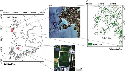
Ground-measured growth and yield and remote sensing data of paddy rice were obtained for two separate sites: one (field area of ~0.4 km²) at the experimental fields of Chonnam National University (CNU), Gwangju, Korea, and another (land area of ~250 km²) in TaeAn, South Chungcheong Province, Korea (Figure 1). The mean annual air temperature and the annual precipitation averaged over the past three decades are 14.3°C and 1395 mm yr⁻¹ in Gwangju and 12.3°C and 1310 mm yr⁻¹ in TaeAn, respectively. In these regions, the East Asian monsoon climate is dominant from June to October in these regions, with more than half of the annual precipitation falling during this time period.

Figure 1. (a) Locations of the two study sites. (b) True-color images of the two study sites: An unmanned aerial vehicle image of a paddy rice field at Chonnam National University (CNU), Gwangju, and a RapidEye image of TaeAn, South Chungcheong Province, Korea. (c) A digitized rice paddy cover map of TaeAn.

Crop growth simulation of paddy rice at the field scale was performed using remotely sensed input data from UAV images taken at the CNU site in 2013. Thirty-day-old seedlings of the rice cultivar Unkwang were transplanted in a paddy field with three separate blocks at this site on 20 May 2013 (day of year (DOY) 140). Nitrogen (N), phosphate (P), and potassium (K) fertilizer with each mass ratio of 0:5:6, 5:5:6, and 11:5:6 was mixed to generate three fertilizer application rates, i.e., 0 kg N ha⁻¹ (plot size of ~511 m²), 50 kg N ha⁻¹ (plot size of ~511 m²), and 115 kg N ha⁻¹ (plot size of ~1387 m²). The three nutrient treatments were applied to each experimental block to investigate spatiotemporal variations of growth conditions and yield variation due to the different applications of N. The nutrient treatment groups were separated by 35-cm-wide cement ways inserted into the soil to a depth of 1 m. Eighty percent of the total N fertilizer was applied by hand spreading 2 days before transplanting, and the rest was used at the active tillering phase of the vegetative stage. P fertilizer was applied as 100% basal dosage, and K fertilizer was applied as 65% basal dosage and 35% tillering phase application. We measured several indicators of plant growth and development, including leaf area index (LAI), using a LI-2200 Plant Canopy Analyzer (LI-COR Inc., Lincoln, NE, USA), and above-ground dry mass (AGDM). LAI was measured with four replications on DOY 172, 190, 206, 220, and 233 for the 0 and 50 kg ha⁻¹ plots and on DOY 159, 168, 172, 178, 183, 190, 198, 206, 220, 231, and 241 for the 115 kg ha⁻¹ plot. Plant samples were collected and dried in an oven at 70°C for 1 week, and then dry mass was measured. The plant samples for AGDM determination were obtained with four replications on DOY 158, 164, 184, 205, 225, and 241 for the 0- and 50-kg ha⁻¹ plots and on DOY 175, 190, 204, and 222 for the 115-kg ha⁻¹ plot. The yield was estimated by multiplying four yield components, which were measured three times in the sample plots based on random sampling at maturity. The yield components were panicle number per m², spikelet number per panicle, percent filled grain, and weight of 1000 grains. Weather data were measured using an automated weather station (WS-GP1, Delta-T Devices, Cambridge, UK).

The TaeAn site was selected, along with the availability of RapidEye satellite images (BlackBridge, Berlin, Germany) for 2010, to perform simulation at the regional scale. According to the Korean Statistical Information Service (KOSIS), two rice cultivars, Samkwang and Hopum, were transplanted at TaeAn between 20 and 27 May 2010, and a N application of 90 kg ha⁻¹ was applied to the fields. The whole regional TaeAn rice yield reported by KOSIS was used as the rice yield representing the study site of interest at the regional scale. Climate data for simulation were obtained from the Korea meteorological weather station located at Seosan (36°46′N, 126°29′E), South Chungcheong Province.

2.2. Model description

The GRAMI-rice model (Ko et al. 2015) was previously framed to project maps of growth and grain yield using remotely sensed images from any given day of interest during the growing season. Unlike detailed crop models, the GRAMI-rice model requires relatively simple input data, including planting date, daily observations of average air temperature and incident solar irradiance, and infrequent observations of remotely sensed VI or LAI data. The GRAMI-rice model is capable of using infrequent remotely sensed data of VI or ground cover to adjust the values of certain model parameters and minimize the error between the remotely sensed data and the model estimates of crop growth. In other words, the model’s parameters and the initial conditions that affect leaf growth and senescence can be adjusted so that the simulated LAI matches the one estimated from remotely sensed crop canopy reflectance (i.e., within-season calibration). This methodology was demonstrated to work well in the model (Maas 1993c; Ko et al. 2005, 2015). In some situations, the model calibrated using remotely sensed crop vegetation can reproduce crop growth conditions more accurately than that calibrated using ground-based observations (Maas 1993c). The model performs four processes for simulating daily paddy rice growth: calculation of (1) growing degree days (GDD), (2) AGDM production, (3) absorption of incident photosynthetically active radiation (PAR) by the canopy, and (4) LAI partitioning or senescence.

The daily change in accumulated GDD (ΔD) is calculated as follows:

(1)

where T is the average daily air temperature (°C) and T_b is a base temperature specific to the crop species. For example, T_b for paddy rice is 12°C. In addition, when T is ≤T_b, the value of ΔD is zero.

The daily increase in AGDM (ΔM) is calculated as follows:

(2)

where is the crop-specific radiation use efficiency (RUE) and Q is the total PAR (MJ m⁻²) absorbed by the crop canopy per day. In the present study, RUE () was estimated as the slope of the regression of dry matter produced and the amount of light energy absorbed over a given time period (Charles-Edwards 1982; Rosenthal and Gerik 1991). The value for paddy rice is 3.49 g MJ⁻¹ (Table 1).

Table 1. GRAMI-rice model parameters for simulation at both the field and regional scales.

Parameter	Symbol	Unit	Value
Radiation use efficiency (RUE)	ε	g MJ^−1	3.49
Light extinction coefficient	k	–	0.6
Specific leaf area	SLA	m^2 g^−1	0.016
Harvest index	HI	–	0.4
Base temperature	Tb	°C	12.0
Leaf area index at transplanting	L0	m^2 m^−2	0.2
Leaf partitioning parameter, A	a	–	0.325
Leaf partitioning parameter, B	b	–	0.00125
Leaf senescence parameter	c	–	0.00125

The amount of incident PAR absorbed by the crop canopy (Q) is calculated as follows:

(3)

where R is the daily incident solar irradiance (MJ m⁻²), is the PAR fraction of the incident solar irradiance, and is a light extinction coefficient that is specific to the given crop. For paddy rice, the value of is 0.6 (Charles-Edwards, Doley, and Rimmington 1986), and the value of is 0.45 (Monteith and Unsworth 2008). The value was estimated according to the relationship between the proportion of daily light energy intercepted by the crop canopy and a range of values. In this estimation, we assumed that the values agreed with the rice canopies of the measured fields at ~0.8, because this is when LAI reached its maximum and the rice canopy covered ~80% of the fields, according to the relationship between the measured normalized difference vegetation index (NDVI) and LAI field data (data not shown). The k value was slightly higher than the range (0.3–0.5) for plants with upright leaves but lower than that (0.7–1.0) for plants with horizontal leaves, as hypothesized by Rosenberg, Blad, and Verma (1983).

The daily increase in LAI from new leaf growth is calculated as follows:

(4)

where is the daily increase in AGDM, P₁ is the fraction of from new leaf growth, and is the specific leaf area of the leaf tissues, which was calculated as 0.016 (Table 3) from the relationship between leaf dry weight and LAI (Rhoads and Bloodworth 1964; Reddy et al. 1989).

Table 2. Pearson’s correlation coefficients (r) and linear regression equations between unmanned aerial vehicle (UAV)-based digital numbers (y) and CROPSCAN reflectance values (x) for wavelengths of interest at different dates during the growing season in 2013.

Day of year	Wavelength (nm)	r	Linear regression
172	450	0.96^ns	y = 0.226x − 4.411
	550	0.94^ns	y = 0.201x − 4.373
	650	0.98^ns	y = 0.224x − 0.047
	800	0.99**	y = 0.427x − 7.863
	880	0.99**	y = 0.578x + 6.285
192	450	0.77^ns	y = 0.191x − 0.351
	550	0.82^ns	y = 0.184x − 1.605
	650	0.92^ns	y = 0.211x − 0.660
	800	0.98^ns	y = 0.311x − 3.616
	880	0.98^ns	y = 0.507x + 1.082
206	450	0.99***	y = 0.433x − 7.315
	550	0.99**	y = 0.429x − 10.996
	650	0.99***	y = 0.438x − 6.492
	800	0.99***	y = 0.576x − 14.43
	880	0.99***	y = 0.887x − 6.821
220	450	0.99**	y = 0.004x − 0.060
	550	0.99**	y = 0.004x − 0.101
	650	0.99***	y = 0.004x − 0.057
	800	0.99***	y = 0.005x − 0.087
	880	0.99***	y = 0.007x − 0.050
233	450	0.99**	y = 0.492x − 2.330
	550	0.99**	y = 0.511x − 4.555
	650	0.99***	y = 0.630x − 3.180
	800	0.99***	y = 0.975x − 8.533
	880	0.99***	y = 1.587x − 2.061

The symbols ** and *** represent significance at the 95% and the 99% probability levels, respectively, and “ns” indicates no significance (n = 3). Criteria for correlations : 0.1–0.3: small; 0.3–0.5: medium; and 0.5–1.0: large.

Table 3. Specifications of the RapidEye satellite system.

Mission characteristic	Information
Number of satellites	5
Spacecraft lifetime	7 years
Orbit altitude	630 km in sun-synchronous orbit
Sensor type	Multispectral push-broom imager
Spectral bands (nm)	Blue (440–510)
	Green (520–590)
	Red (630–685)
	Red edge (690–730)
	Near-infrared (760–850)
Ground sampling distance (nadir)	6.5 m
Pixel size (ortho-rectified)	5 m
Swath width	77 km
Onboard data storage	Up to 1500 km of image data per orbit
Revisit time	Daily (off nadir), 5.5 days (at nadir)
Image capture capacity	4 million km^2 per day
Dynamic range	Up to 12 bits

Finally, the dimensionless leaf-partitioning fraction () was calculated as follows:

(5)

where a and b are parameters that control the magnitude and shape of the fraction, and D is the cumulative GDD. In Equation (4), P₁ functions to reduce the partitioning of new dry mass to new leaf growth as the crop approaches its reproductive phase.

The leaf senescence used in the model was formulated by assuming that the leaves start to senesce after attaining the maximum LAI and that the senescence rate varies depending on plant genetic traits and environmental conditions. These aspects were incorporated into the model by re-parameterizing the parameter c (see Table 1), according to within-season calibration (for detailed information, see Maas 1993a, 1993b).

The GRAMI model incorporates a within-season calibration procedure that calibrates simulated crop growth based on actual observations (Figure 2). The model produces a growth simulation that consists of daily estimates of crop state variables, such as LAI and AGDM, from daily climate input data, such as air temperate and solar irradiance, and then the simulated LAI or VI values are compared with the corresponding observed corresponding values. The two data sets are compared and the calibration procedure is initiated if the data sets do not match completely. In this procedure, the parameter values that control the response of the model to the climate data are revised, and the model is restarted to produce a growth simulation with the new parameter values. The new simulation is also compared with the observed LAI or VI values to determine whether the parameter values require further adjustment (Maas 1993b). Although the rice model is capable of using five VIs (i.e., enhanced vegetation index (EVI); modified triangular vegetation index (MTVI); NDVI; optimized soil-adjusted vegetation index (OSAVI); and renormalized difference vegetation index (RDVI)) as inputs for the within-season calibration, only NDVI was used in the current study as it is considered a more representative VI than the others.

Figure 2. Schematic representation of crop growth mapping using the GRAMI-rice model. NDVI, LAI, and AGDM represent normalized difference vegetation index, leaf area index, and above-ground dry mass, respectively.

Four parameters (L₀, a, b, and c) are used to simulate crop growth in the model, and the previously determined initial values of the four parameters for paddy rice (Ko et al. 2015) are 0.2, 0.325, 0.00125, and 0.00125, respectively (Table 1). The initial value of LAI (L₀) at crop emergence is determined in the first step. The parameters of a, b, and c are then re-parameterized systematically during the model calibration, as described by Maas (1993a, 1993b).

2.3. Remote sensing data for mapping crop growth and yield

The crop simulation procedure was performed iteratively for each pixel of field VI data using the GRAMI model to project maps of crop growth and yield (see Figure 2). A crop information delivery system (CIDS) was previously designed to deliver information on crop growth and yield with predictive maps using the GRAMI model with remote sensing data inputs (refer to Ko et al. 2015). The CIDS is an extended version of GRAMI, capable of simulating pixel-based crop growth and yield maps using remotely sensed imageries. The core component of the CIDS is a version of the GRAMI-rice model that was parameterized and evaluated for its capability to reproduce rice field conditions. In order to simulate maps of crop growth and yield, the CIDS needs to use pixel-based remotely sensed data and climate data as inputs. The CIDS can use climate data from either one station or multiple stations, depending on the situation. The GRAMI model simulates the crop in each pixel using both input data.

Remotely sensed images from the two different locations mentioned earlier (see Figure 1) were used to perform these simulation studies, and climate conditions were represented with point climate data for both locations. Remotely sensed information pertaining to rice canopy growth (i.e., scene reflectance) at the CNU site was acquired using a Miniature Multiple Camera Array (Mini-MCA6; Tetracam Inc., Chatsworth, CA, USA) that was mounted on a UAV. The UAV was previously constructed with eight propellers, a radius of 515 mm, a height of 495 mm, and a total weight of 5 kg (Jeong et al. 2016). The UAV could fly at an altitude of up to approximately 1000 m and hover for 15–20 min. The Mini-MCA6 weighs 750 g and has horizontal and vertical viewing angles of 38.26° and 30.97°, respectively. The field of view of the camera is 208 × 166 m, and the ground resolution of a pixel is approximately 16 cm at an altitude of 300 m. The Mini-MCA consisted of six spectral sensors with wavebands of 450, 550, 650, 800, 830, and 880 nm, and images from each individual sensor comprised 1280 × 1024 pixels. Single-scene images acquired at ~300 m above the ground were taken at around noon, between 12:10 and 13:10, due to the need to minimize the change of reflectance due to the sun angle and shadow effects on multiple days of the year during the crop season of 2013: DOY 172, DOY 192, DOY 206, DOY 220, and DOY 233. These dates were selected according to the significant rice growth stages and were mostly on clear days.

Radiometric and geometric corrections were applied to the acquired UAV images. To make the radiometric corrections of the UAV images, calibration targets were placed on a flat surface next to the study site. Each target was made from an aluminum plate (2.4 × 2.4 m each) and was marked with nonreflective black, gray, and white paint. The reflectance values derived from the UAV system were estimated from linear relationships between the digital numbers of UAV images and ground reflectance (Table 2), according to the empirical line method, and the ground reflectance values were measured using a portable multispectral radiometer (CROPSCAN Inc., Rochester, MN, USA). Because raw UAV images contain no geographic information, we also conducted geo-referenced image processing, using a number of ground control points, to match pixels in images from different dates. This process was used for the geometric correction of the images, and the entire image correction process was performed using IDL/ENVI software (EXELIS Inc., Rochester, NY, USA).

We also used satellite remotely sensed images taken by RapidEye (BlackBridge), which collects 4 million square kilometers of data per day with a 6.5 m ground resolution (Table 3). RapidEye satellite images comprise five spectral wavebands (red, green, blue, red edge, and near-infrared) and are provided commercially with two processing levels: (1) geometrically uncorrected images and (2) radiometrically and geometrically corrected images (BlackBridge 2015). For the present study, we obtained radiometrically and geometrically corrected RapidEye images of the TaeAn site that were acquired on DOY 152, 174, 220, and 250 in 2010. These images were further processed using the Fast Line-of-sight Atmospheric Analysis of Spectral Hypercubes atmospheric correction method (Adler-Golden et al. 1998), and paddy areas were identified in the corrected RapidEye images using a digitized paddy cover map from the Ministry of Agriculture, Food and Rural Affairs, Korea (Figure 1(c)).

NDVI images were then produced using the red and near-infrared reflectance values of the remotely sensed images (Figures 3 and 4). The NDVI maps of the rice field were specifically resampled to generate maps with a ground resolution of 1 m. This procedure was performed because we assumed that the spatial resolution of 1.0 m was the best option for analyzing crop growth and development at a plant canopy scale. Average values from each NDVI image were extracted to assemble a sequential set of NDVI values for each study field, and the NDVI images were also utilized as inputs for the GRAMI-rice model to simulate two-dimensional growth and estimate grain yield.

Figure 3. Time series maps (a–e) of the normalized difference vegetation index (NDVI) of paddy rice fields at Chonnam National University, Gwangju, Korea, in 2013. The NDVI maps were generated for several days of the year (DOY): (a) DOY 172, (b) DOY 192, (c) DOY 206, (d) DOY 220, and (e) DOY 233.

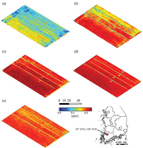
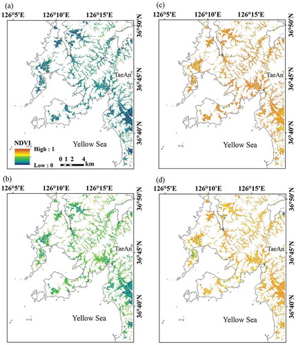
Figure 4. Time series maps (a–d) of the normalized difference vegetation index (NDVI) of classified paddy rice fields at TaeAn, South Chungcheong Province, Korea, in 2010. The NDVI maps were generated for several days of the year (DOY): (a) DOY 152, (b) DOY 174, (c) DOY 220, and (d) DOY 250.

2.4. Statistical evaluation

For model evaluation, the mean values of simulated crop yield, AGDM, LAI, and NDVI were compared with the measured values. We used the paired t-test (SAS v9.2, SAS Institute, Cary, NC, USA) and the three statistical indices of root mean square error (RMSE, Equation (6)), mean absolute error (MAE, Equation (7)), and model efficiency (ME, Equation (8); Nash and Sutcliffe 1970):

(6)

(7)

(8)

where S_i is the ith simulated value, M_i is the ith measured value, M_avg is the averaged measured value, and n is the whole number of data. ME values are equivalent to the coefficient of determination (R²) if the values fall around the 1:1 line of simulated versus measured data, but ME is generally lower than R² and can be negative when the predictions are very biased.

3. Results

At the field scale, the GRAMI-rice model reproduced our field observations of paddy rice growth and grain yield, using UAV-based spatial NDVI data of paddy rice fields at CNU (see Figure 3), and the accuracy of the model’s simulations was examined. We found that the GRAMI-rice model reproduced our field observations of paddy rice growth (i.e., NDVI, LAI, and AGDM) with reasonable accuracy (Figure 5), although there were some disagreements between the field measurements and the simulations of AGDM (i.e., DOY 190 and 240 for 0 kg of N ha⁻¹ and DOY 190 for 50 kg of N ha⁻¹) and NDVI (i.e., DOY 239). For NDVI, the RMSE and MAE values for the fields with the 0, 50, and 115 kg ha⁻¹ N applications ranged from 0.03 to 0.07 and 0.02 to 0.03, whereas the ME values were 0.97, 0.89, and 0.97, respectively (Table 4). For LAI, the RMSE values for the fields with the 0, 50, and 115 kg ha⁻¹ N applications were 0.26, 0.33, and 0.38 m² m⁻², the MAE values were 0.15, 0.25, and 0.26 m² m⁻², and the ME values were 0.94, 0.91, and 0.95, respectively. For AGDM, the RMSE values for the fields with the 0, 50, and 115 kg ha⁻¹ N applications were 18.13, 9.67, and 2.65 kg ha⁻¹, the MAE values were 6.75, 2.71, and 2.44 kg ha⁻¹, and the ME values were 0.86, 0.96, and 0.99, respectively.

Table 4. Error statistics (root mean square error, RMSE, mean absolute error, MAE, and model efficiency, ME) for comparisons between simulated and measured normalized difference vegetation index (NDVI), leaf area index (LAI), and above-ground dry mass (AGDM) values under nitrogen applications of 0, 50, and 115 kg ha⁻¹ at Chonnam National University, Gwangju, Korea, in 2013.

Nitrogen application (kg ha^−1)	NDVI			LAI			AGDM
	RMSE	MAE	ME	RMSE (m^2 m^−2)	MAE (m^2 m^−2)	ME	RMSE (kg ha^−1)	MAE (kg ha^−1)	ME
0	0.030	0.018	0.972	0.259	0.149	0.948	18.126	6.751	0.861
50	0.066	0.024	0.885	0.331	0.248	0.913	9.671	2.714	0.958
115	0.065	0.026	0.889	0.375	0.259	0.947	2.653	2.437	0.995

Figure 5. Simulated and measured values of normalized difference vegetation index (NDVI), leaf area index (LAI), and above-ground dry mass (AGDM) of paddy rice during the growing season in 2013 at Chonnam National University, Gwangju, Korea, under nitrogen (N) applications of 0, 50, and 115 kg ha⁻¹. The data points and vertical error bars represent the mean measured values ±1 SE (n = 4).

There were no significant statistical differences between the model’s simulated field-scale grain yields and our measured field values for any of the 0, 50, or 115 kg ha⁻¹ N application levels (Figure 6) according to paired t-tests (p = 0.45, p = 0.27, and p = 0.52, respectively). In addition, the RMSE values for the fields with the 0, 50, and 115 kg ha⁻¹ N applications were 340.1, 574.6, and 251.7 kg ha⁻¹, the MAE values were 254.9, 430.5, and 144.5 kg ha⁻¹, and the ME values were 0.24, −0.54, and 0.18, respectively.

Figure 6. Comparison of simulated and measured grain yields of paddy rice during the growing season in 2013 at Chonnam National University, Gwangju, Korea, under nitrogen (N) applications of 0, 50, and 115 kg ha⁻¹. The p values were obtained from paired t-tests (α = 0.05). The vertical error bars represent ±1 SE of the simulated and measured mean values (n = 3).

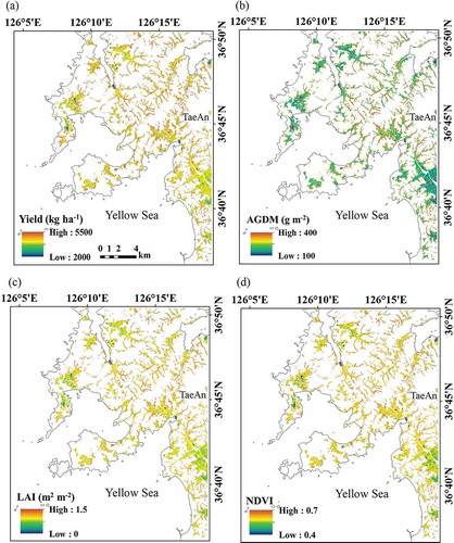
At the regional scale, simulation was performed for the TaeAn site using RapidEye satellite NDVI images (5 m pixel resolution). Maps of the rice growth variables and grain yield prediction were projected at 57 days after planting, which corresponded to the booting stage (Figure 7). The predicted NDVI, LAI, AGDM, and grain yield values ranged from 0.6 to 0.8, 1.9 to 3.0 m² m⁻², 200 to 500 g m⁻², and 3697.2 to 5548.4 kg ha⁻¹, respectively. We found that the simulated grain yields of the classified paddy rice fields at TaeAn, with a mean value of 4622.8 kg ha⁻¹ ± 1 SD of 850.3 kg ha⁻¹, were in correspondence with the reported grain yield value of 4290 kg ha⁻¹. The absolute error was 332.8 kg ha⁻¹ while the relative error was 0.08.

Figure 7. Maps of (a) grain yield; (b) above-ground dry mass, AGDM; (c) leaf area index, LAI; and (d) normalized difference vegetation index, NDVI, of classified paddy fields in TaeAn, South Chungcheong Province, Korea, at 57 days after transplanting in 2010.

4. Discussion

In the present study, we evaluated the ability of the GRAMI-rice model to simulate crop growth and grain yield at both the field scale and the regional scale using UAV images and RapidEye satellite images, respectively. We found that the recently extended GRAMI-rice model, which uses remotely sensed data, successfully monitored canopy growth and accurately estimated grain yield of paddy rice via map projections at various spatial resolutions. The current simulation study result at the field scale specifically demonstrated that it is possible to simulate spatiotemporal variations of crop growth and yield variation due to different N applications in the field. The simulation result using the RapidEye satellite imageries also showed that the GRAMI-rice model can reproduce spatiotemporal variations of rice growth conditions and yield due mainly to different field conditions at the regional scale with the spatial resolution of a resampling pixel resolution of 5 m and a swath width of 77 km. In addition, our findings also verified the ability of the GRAMI-rice model to use LAI or VI data to minimize the error between simulated and observed canopy growth variables (Ko et al. 2015).

The ability to perform within-season calibration allows the GRAMI model to reproduce crop growth and grain yields using remotely sensed data, a process that requires minimal environmental input data (Maas et al., 1993b; Ko et al. 2005), and the method has been validated for several staple crops using inputs from different remote sensing platforms (Maas 1993c; Moran, Maas, and Pinter 1995; Doraiswamy et al. 2003; Padilla et al. 2012; Yeom, Ko, and Kim 2015). Thus, the model should be useful for monitoring crop growth conditions and determining grain yield. However, because of the model’s strong dependence on remote sensing data, some limitations exist. Therefore, we hereafter discuss the dependence of the GRAMI-rice model on the timing, spatial resolution, and area coverage of the required remotely sensed data.

The current GRAMI model estimates LAI from VI using an empirical modeling approach when remotely sensed data are used as an input. Previously, VI has been used as a representative indicator of the canopy conditions of crops and has provided valuable information for determining crop growth and grain yield (Zarco-Tejada, Ustin, and Whiting 2005; Bolton and Friedl 2013; Johnson 2014). However, VI data collected too early or too late during the growing season may provide poor estimates of the actual canopy conditions. Ko et al. (2015), for example, reported that the GRAMI model was incapable of reproducing observations when single data points were used as input but that acceptable agreement between the simulation and field measurements could be obtained when four evenly distributed data points were used to represent crop conditions over the growing season. Therefore, the timing of remote sensing data acquisition can be crucial for increasing the model’s accuracy.

At field scales, UAV remote sensing systems can be used to monitor crop growth conditions easily and flexibly with high spatial resolution (Hunt et al. 2010; Jannoura et al. 2015; Ko et al. 2015), and obtaining UAV remote sensing images is less limited, in terms of acquisition timing, than obtaining satellite images. UAVs can provide remote sensing data for running the GRAMI model more securely than any other remote sensing platform as the operating costs are decreasing, increasing the availability of these systems for use in many areas and countries. The limitation of using UAV remote sensing systems is that UAVs are less suitable than satellite platforms in their capacities of broader coverage for regional scale simulations using the GRAMI model. In cases when satellite images are not available, application of the GRAMI model may be unable to provide regional scale simulations. Thus, for application of the GRAMI-rice model at the regional scale, this constraint should be satisfied with appropriate acquisition of satellite images, in terms of number and timing, for example, evenly distributed at four times representing crop conditions over the growing season (Ko et al. 2015).

High spatial resolution and wide coverage area are conflicting criteria for crop monitoring missions that use satellite remote sensing. Although the GRAMI-rice model can simulate crop growth for large areas, it is restricted in simulation performance because of the inaccurate representation of crop canopy conditions that results from the coarse spatial resolution of satellite images with mixed pixels. The spatial resolution of individual satellite systems depends on the orbital height, swath width, and revisit time of the satellites (Wertz and Larson 1999). However, it is also difficult to obtain data over a broad area within a short temporal period using satellites with very high spatial resolutions (e.g., GeoEye-2, KOMPSAT-3, and WorldView-3) because such systems are generally designed to view relatively narrow swaths. In addition, some other satellite systems, such as MODIS, have the advantage of higher revisit rates and broader area coverage; however, they are incapable of measuring the precise spectral characteristics of homogeneous crop field conditions due to their low spatial resolution, i.e., 250 m or less (Ozdogan and Woodcock 2006). Therefore, it is worthwhile to define the optimum spatial resolution of satellite remote sensing data for the GRAMI-rice model so that the spectral characteristics of crop scenes can be classified with homogeneous conditions from the mixed satellite image pixels without complicated data processing. The GRAMI-rice model could then be utilized to produce cost-effective CIDS, using satellite remote sensing data with rapid data processing. In this context, RapidEye, which has a resampling pixel resolution of 5 m and a swath width of 77 km, would be one of the optimal resolution satellites for monitoring and mapping regions of interest (Kim and Yeom 2015). Although solving the issue of spectral resolution is out of the scope of the current study, it would be worthwhile to investigate the optimum ranges of spectral resolution for the wavelengths applied to determine vegetation indices.

5. Conclusion

We demonstrated that the GRAMI-simulated rice growth variables NDVI, LAI, and AGDM were in statistical agreement with corresponding field measurements and that the model was capable of reproducing accurate grain yield measurements. In addition, the results of this study demonstrated that the model’s map projections of paddy rice growth and grain yield could accurately represent the spatial variation of observed field conditions from RapidEye satellite images. Thus, we demonstrated the potential use of the GRAMI-rice model and satellite images for mapping the growth and grain yield of rice at both field and regional scales of interest within the coverages of a UAV or the RapidEye satellite. The GRAMI-rice model can provide a reasonably dependable simulation of seasonal variations in rice growth and grain yield at different spatial scales. Nevertheless, further studies are needed to extend the GRAMI-rice model to simulate growth and production for much larger regions such as entire countries and/or continents at high spatial scales.

Acknowledgements

The present study was supported by the Basic Science Research Program through the National Research Foundation of Korea (NRF), funded by the Ministry of Education, Science, and Technology (NRF-2011-0009827 and NRF-2015R1D1A1A01057586).

Disclosure statement

No potential conflict of interest was reported by the authors.

Additional information

Funding

This present study was supported by the Basic Science Research Program through the National Research Foundation of Korea, funded by the Ministry of Education, Science and Technology [NRF-2011-0009827 and NRF-2015R1D1A1A01057586].

References

- Adler-Golden, S., A. Berk, L. S. Bernstein, S. Richtsmeier, P. K. Acharya, M. W. Matthew, G. P. Anderson, C. L. Allred, L. S. Jeong, and J. H. Chetwynd 1998. “FLAASH, A MODTRAN4 Atmospheric Correction Package for Hyperspectral Data Retrievals and Simulations.” Proceedings of the 7th Annual JPL Airborne Earth Science Workshop, December 9–14. https://www.researchgate.net/profile/Bo-Cai_Gao/publication/
- Aparicio, N., D. Villegas, J. Casadesus, J. L. Araus, and C. Royo. 1999. “Spectral Vegetation Indices as Nondestructive Tools for Determining Durum Wheat Yield.” Agronomy Journal 92 (1): 83–91. doi:10.2134/agronj2000.92183x.
- Asrar, G., E. T. Kanemasu, R. D. Jackson, and P. J. Pinter. 1985. “Estimation of Total Above-Ground Phytomass Production Using Remotely Sensed Data.” Remote Sensing of Environment 17 (3): 211–220. doi:10.1016/0034-4257(85)90095-1.
- BlackBridge. 2015. “Satellite imagery product specifications, Version 6.1.” Accessed September 29, 2015. http://blackbridge.com/rapideye/upload/RE_Product_Specifications_ENG.pdf
- Bolton, D. K., and M. A. Friedl. 2013. “Forecasting Crop Yield Using Remotely Sensed Vegetation Indices and Crop Phenology Metrics.” Agricultural and Forest Meteorology 173: 74–84. doi:10.1016/j.agrformet.2013.01.007.
- Charles-Edwards, D. A. 1982. Physiological Determinants of Crop Growth. Orlando, FL: Academic Press.
- Charles-Edwards, D. A., D. Doley, and G. M. Rimmington. 1986. Modeling Plant and Development. Orlando, FL: Academic Press.
- Doraiswamy, P. C., S. Moulin, P. W. Cook, and A. Stern. 2003. “Crop Yield Assessment from Remote Sensing.” Photogrammetric Engineering Remote Sensing 69 (6): 665–674. doi:10.14358/PERS.69.6.665.
- Hunt, E. R., W. D. Hively, S. J. Fujikawa, D. S. Linden, C. S. Daughtry, and G. W. McCarty. 2010. “Acquisition of NIR-Green-Blue Digital Photographs from Unmanned Aircraft for Crop Monitoring.” Remote Sensing 2 (1): 290–305. doi:10.3390/rs2010290.
- Jannoura, R., K. Brinkmann, D. Uteau, C. Bruns, and R. G. Joergensen. 2015. “Monitoring of Crop Biomass Using True Color Aerial Photographs Taken from a Remote Controlled Hexacopter.” Biosystems Engineering 129: 341–351. doi:10.1016/j.biosystemseng.2014.11.007.
- Jeong, S., J. Ko, M. Kim, and J. Kim. 2016. “Construction of an Unmanned Aerial Vehicle Remote Sensing System for Crop Monitoring.” Journal of Applied Remote Sensing 10 (2): 026027. doi:10.1117/1.jrs.10.026027.
- Johnson, D. M. 2014. “An Assessment of Pre- and Within-Season Remotely Sensed Variables for Forecasting Corn and Soybean Yields in the United States.” Remote Sensing of Environment 141: 116–128. doi:10.1016/j.rse.2013.10.027.
- Jones, J. W., G. Hoogenboom, C. H. Porter, K. J. Boote, W. D. Batchelor, L. A. Hunt, P. W. Wilkens, U. Singh, A. J. Gijsman, and J. T. Ritchie. 2003. “The DSSAT Cropping System Model.” European Journal of Agronomy 18: 235–265. doi:10.1016/S1161-0301(02)00107-7.
- Kim, H., and J. Yeom. 2015. “sensitivity Of Vegetation Indices To Spatial Degradation Of Rapideye Imagery For Paddy Rice Detection: A Case Study Of South Korea.” Giscience & Remote Sensing 52: 1-17. doi: 10.1080/15481603.2014.1001666.
- Ko, J., S. Jeong, J. Yeom, H. Kim, J. O. Ban, and H. Y. Kim. 2015. “Simulation and Mapping of Rice Growth and Yield Based on Remote Sensing.” Journal of Applied Remote Sensing 9 (1): 096067–096067. doi:10.1117/1.JRS.9.096067.
- Ko, J., S. J. Maas, R. J. Lascano, and D. Wanjura. 2005. “Modification of the GRAMI Model for Cotton.” Agronomy Journal 97 (5): 1374–1379. doi:10.2134/agronj2004.0267.
- Labus, M. P., G. A. Nielsen, R. L. Lawrence, R. Engel, and D. S. Long. 2002. “Wheat Yield Estimates Using Multi-Temporal NDVI Satellite Imagery.” International Journal of Remote Sensing 23 (20): 4169–4180. doi:10.1080/01431160110107653.
- Ma, B. L., L. M. Dwyer, C. Costa, E. R. Cober, and M. J. Morrison. 2001. “Early Prediction of Soybean Yield from Canopy Reflectance Measurements.” Agronomy Journal 93 (6): 1227–1234. doi:10.2134/agronj2001.1227.
- Maas, S. J. 1993a. “Parameterized Model of Gramineous Crop Growth: I. Leaf Area and Dry Mass Simulation.” Agronomy Journal 85 (2): 348–353. doi:10.2134/agronj1993.00021962008500020034x.
- Maas, S. J. 1993b. “Parameterized Model of Gramineous Crop Growth: II. Within-Season Simulation Calibration.” Agronomy Journal 85 (2): 354–358. doi:10.2134/agronj1993.00021962008500020035x.
- Maas, S. J. 1993c. “Within-Season Calibration of Modeled Wheat Growth Using Remote Sensing and Field Sampling.” Agronomy Journal 85 (3): 669–672. doi:10.2134/agronj1993.00021962008500030028x.
- Monteith, J. L., and M. H. Unsworth. 2008. Principles of Environmental Physics. 3rd ed. Burlington, MA: Academic Press.
- Moran, M. S., S. J. Maas, and P. J. Pinter Jr. 1995. “Combining Remote Sensing and Modeling for Estimating Surface Evaporation and Biomass Production.” Remote Sensing Reviews 12 (3–4): 335–353. doi:10.1080/02757259509532290.
- Moulin, S., A. Bondeau, and R. Delecolle. 1998. “Combining Agricultural Crop Models and Satellite Observations: From Field to Regional Scales.” International Journal of Remote Sensing 19 (6): 1021–1036. doi:10.1080/014311698215586.
- Nash, J. E., and J. V. Sutcliffe. 1970. “River Flow Forecasting through Conceptual Models: Part I. A Discussion of Principles.” Journal of Hydrology 10 (3): 282–290. doi:10.1016/0022-1694(70)90255-6.
- Ozdogan, M., and C. E. Woodcock. 2006. “Resolution Dependent Errors in Remote Sensing of Cultivated Areas.” Remote Sensing of Environment 103: 203–217. doi:10.1016/j.rse.2006.04.004.
- Padilla, F. L. M., S. J. Maas, M. P. González-Dugo, F. Mansilla, N. Rajan, P. Gavilán, and J. Domínguez. 2012. “Monitoring Regional Wheat Yield in Southern Spain Using the GRAMI Model and Satellite Imagery.” Field Crops Research 130: 145–154. doi:10.1016/j.fcr.2012.02.025.
- Reddy, V. R., B. Acock, D. N. Baker, and M. Acock. 1989. “Seasonal Leaf Area–Leaf Weight Relationships in the Cotton Canopy.” Agronomy Journal 81: 1–4. doi:10.2134/agronj1989.00021962008100010001x.
- Rhoads, F. M., and M. E. Bloodworth. 1964. “Area Measurement of Cotton Leaves by Dry Weight Method.” Agronomy Journal 56: 520–522. doi:10.2134/agronj1964.00021962005600050024x.
- Rosenberg, N. J., B. L. Blad, and S. B. Verma. 1983. Microclimate: The Biological Environment. 2nd ed. New York: John Wiley & Sons.
- Rosenthal, W. D., and T. J. Gerik. 1991. “Radiation Use Efficiency among Cotton Cultivars.” Agronomy Journal 83: 655–658. doi:10.2134/agronj1991.00021962008300040001x.
- Rosenthal, W. D., R. L. Vanderlip, B. S. Jackson, and G. F. Arkin. 1989. SORKAM: A Grain Sorghum Crop Model. Miscellaneous Publication MP-1669. College Station: Texas Agricultural Experiment Station.
- Stockle, C. O., M. Donatelli, and R. Nelson. 2003. “Cropsyst a Cropping System Model.” European Journal Agronomy 18: 289–307. doi:10.1016/S1161-0301(02)00109-0.
- Wertz, J. R., and W. J. Larson. 1999. Space Mission Analysis and Design. 3rd ed. El Segundo: Space Technology Library.
- Wilkerson, G. G., J. W. Jones, K. J. Boot, and J. W. Mishoe. 1985. SOYGRO V5.0: Soybean Crop Growth and Yield Model. Technical Documentation. Gainesville, FL: Univ. of Florida.
- Williams, J. R., C. A. Jones, J. R. Kiniry, and D. A. Spanel. 1989. “The EPIC Crop Growth Model.” Transactions of the ASAE 32: 497–511. doi:10.13031/2013.31032.
- Yeom, J., J. Ko, and H. Kim. 2015. “Application of GOCI-Derived Vegetation Index Profiles to Estimation of Paddy Rice Yield Using the GRAMI Rice Model.” Computers and Electronics in Agriculture 118: 1–8. doi:10.1016/j.compag.2015.08.017.
- Zarco-Tejada, P. J., S. L. Ustin, and M. L. Whiting. 2005. “Temporal and Spatial Relationships between Within-Field Yield Variability in Cotton and High-Spatial Hyperspectral Remote Sensing Imagery.” Agronomy Journal 97: 641–653. doi:10.2134/agronj2003.0257.
- Zhao, D., K. R. Reddy, V. G. Kakani, J. J. Read, and S. Koti. 2007. “Canopy Reflectance in Cotton for Growth Assessment and Lint Yield Prediction.” European Journal of Agronomy 26 (3): 335–344. doi:10.1016/j.eja.2006.12.001.