Sensitivity analysis and accuracy assessment of the land transformation model using cellular automata

Abstract

This study evaluates the effects of cellular automata (CA) with different neighborhood sizes on the predictive performance of the Land Transformation Model (LTM). Landsat images were used to extract urban footprints and the driving forces behind urban growth seen for the metropolitan areas of Tehran and Isfahan in Iran. LTM, which uses a back-propagation neural network, was applied to investigate the relationships between urban growth and the associated drivers, and to create the transition probability map. To simulate urban growth, the following two approaches were implemented: (a) the LTM using a top-down approach for cell allocation grounding on the highest values in the transition probability map and (b) a CA with varying spatial neighborhood sizes. The results show that using the LTM-CA approach increases the accuracy of the simulated land use maps when compared with the use of the LTM top-down approach. In particular, the LTM-CA with a 7 × 7 neighborhood size performed well and improved the accuracy. The level of agreement between simulated and actual urban growth increased from 58% to 61% for Tehran and from 39% to 43% for Isfahan. In conclusion, even though the LTM-CA outperforms the LTM with a top-down approach, more studies have to be carried out within other geographical settings to better evaluate the effect of CA on the allocation phase of the urban growth simulation.

Keywords:

• Land Transformation Model
• cellular automata
• accuracy assessment
• sensitivity analysis

1. Introduction

Urban land consumption changes the ecosystem functions with substantial consequences for humans, biodiversity, and natural resources (Grekousis and Mountrakis 2015). Monitoring and modeling land use and land cover (LULC) changes are thus essential for understanding the dynamic processes in cities (Serneels and Lambin 2001; Corner, Dewan, and Chakma 2014). It is key for LULC models to produce accurate and reliable simulation maps of past and future urban growth (Veldkamp and Lambin 2001). An extensive body of literature has been produced dealing with the importance of LULC changes in relation to the environment, biodiversity, and climate change (e.g., Pijanowski et al. 2002; Verburg et al. 2002; Lambin, Geist, and Lepers 2003; Dewan and Yamaguchi 2009b; Thapa and Murayama 2011; Dewan et al. 2012; Taubenböck et al. 2012; Grekousis, Mountrakis, and Kavouras 2016). Consistently, these studies have confirmed the importance of using accurate LULC maps and models for environmental planning and land use purposes. More precisely, LULC maps support sustainable and environment-oriented decision-making; helping to avoid the unwanted effects of human activity on vulnerable natural resources. In addition, they can also be utilized to aid the land management aspects of urban expansion.

Technological developments such as remote sensing, geographic information systems, and the use of data on a detailed spatial and temporal scale, have together led to the development of an increasing number of LULC change models. Such models range from cellular automata (CA)and statistical techniques (e.g., logistic regression and multivariate adaptive spline regression) to machine learning and data mining algorithms (e.g., artificial neural networks, ANNs), as well as support vector machines (Pijanowski et al. 2002; Yang, Li, and Shi 2008; Corner, Dewan, and Chakma 2014; Mozumder and Tripathi 2014; Azari et al. 2016; Newman, Lee, and Berke 2016). Previous studies have reported on the highly complex relationships that exist between LULC change and the driving forces behind such change, revealing them to be exceedingly nonlinear in nature (e.g., Pijanowski et al. 2002; Almeida et al. 2008; Mozumder and Tripathi 2014). These nonlinearities can be properly modeled by means of nonparametric techniques such as ANNs (e.g., Li and Yeh 2001; Grekousis, Manetos, and Photis 2013; Mozumder and Tripathi 2014), which are well known for their computational speed, representational flexibility, and excellent levels of performance when compared with conventional statistical techniques (Fischer 2006; Hagenauer and Helbich 2012). For these reasons, ANNs have become integral to many land use studies (e.g., Shafizadeh-Moghadam et al. 2015; Tayyebi et al. 2016; Tayyebi and Pijanowski 2014).

Pijanowski et al. (2002) developed the LTM, which utilizes a back-propagation ANN to explore associations between input variables (i.e., driving forces) and output variables (i.e., cells experiencing land use change). Within the LTM, the estimation and allocation routines used to calculate the number of cells that have experienced land use change can be described as follows. The amount of change in the model can be identical to the number of changed cells during the previous time interval, or be calculated by referring to the population rate of a given region and over a given period of time. An alternative approach to determining the quantity of cells likely to change is the Markov chain (Ozturk 2015), which calculates the transition probability between every pair of cell states in the form of a transition probability matrix. While this technique has been widely utilized within land change modeling circles (e.g., Pontius and Malanson 2005; Olmedo et al. 2015), it has also been criticized for its nonspatial nature (Boerner et al. 1996). To allocate land use change, Pijanowski et al. (2002) have developed a cell allocation model in which cells with the highest likelihood values are supposed to change first. This means target cells are assigned to the maximum likelihood values on a transition probability map, thereafter generating a simulated map. This process is referred to as a top-down cell allocation process. At the end, by overlaying the simulated maps onto the observed maps, an error map can be produced.

In spite of the fact that the cell allocation used by LTM seems logical and the results obtained by the model have been encouraging (e.g., Pijanowski et al. 2002; Shafizadeh-Moghadam et al. 2015; Newman, Lee, and Berke 2016), the model disregards the influence of neighboring cells, something that CA does take into account. CA is basically a neighborhood function which reflects the first law of geography, that is, that “everything is related to everything else, but near things are more related than distant things” (Tobler 1970). Alluding to this law, CA assumes that if a target cell has already been developed, the chance of a neighboring cell also developing is increased. CA is a rather simple approach based on predefined transition rules, but is able to create complex land use patterns (White and Engelen 1993; Clarke and Gaydos 1998; Batty, Xie, and Sun 1999), as transition rules exhibited in the form of neighborhood functions are used to model cell changes (Li and Yeh 2000). Past studies have developed different CA models to investigate LULC change (White and Engelen 1993; Clarke and Gaydos 1998; Wu and Webster 1998; Batty, Xie, and Sun 1999); for example, CA has been employed both in isolation and in combination with other methods such as ANNs (e.g., Li and Yeh 2001), SVMs (e.g., Yang, Li, and Shi 2008), logistic regressions (e.g., Lin et al. 2011), and random forests (e.g., Kamusoko and Gamba 2015). While ANN is a nonspatial model used for modeling the relationship between urban growth and its drivers, CA is spatially explicit, and is able to account for the influence of neighborhood effects as part of the cell allocation process. However, tuning the CA and defining neighborhood functions so as to capture the complexity of urban dynamics is still a challenging task since it incorporates a high-dimensional search space (Blecic, Cecchini, and Trunfio 2014).

When referring to the numerous CA applications, and when considering the successful implementations of Land Transformation Model (LTM), using a top-down approach, one pressing question remains: Which approach produces more accurate LULC simulations? This study seeks to answer this question by comparing the effectiveness of LTM with and without CA. More specifically, it investigates whether implementing the CA model during the cell allocation process increases the accuracy of simulated land use maps produced by the LTM. To the best of our knowledge, no study has yet explored this issue.

2. Study area and data

2.1 Study area

In this paper, we used two metropolitan areas, namely Tehran and Isfahan, in Iran as case studies (Figure 1). While the former represents a megacity, the latter is among the large cities in Iran which manifests different urban growth dynamics and patterns. Therefore, both cities are an excellent choice for the present analyses.

Figure 1. Study areas (false color images of Landsat 8 for the year 2014).

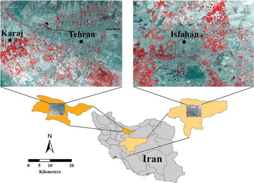
Tehran, the capital of Iran, is the country’s most populated city. Located at 35° 45´ N and 51° 30´ E, the city incorporates 22 districts which cover 700 km² (Madanipour 2006). Nowadays, according to the official census, over 8 million people live in the city (Census Information 2011). Tehran is the primary destination for immigrants, as it is the focus of Iran’s commercial, financial, cultural, and educational activities. Tehran’s morphology is characterized by high-rise buildings, vertical and horizontal growth and a high-density population. Not only have cropland and green spaces been converted to built-up areas but also hilly areas have been turned into construction sites. Based on this trend, it is expected that any nonurban land that still exists between Tehran and Karaj¹ will soon disappear, and that both cities will eventually merge.

The second study area was Isfahan. Isfahan is located at 32°38′ N and 51°38′ E next to the Zagros mountain in Central Iran. The city covers 340 km² (Figure 1). The height of the city ranges from 1550 m to 2232 m. Isfahan is divided into a southern and northern part through the Zayanderood river. This river has been considered as a leading urban growth factor (Bihamta et al. 2015). Due to the historical and economic values, Isfahan is one of the important cities in Iran attracting a large number of tourists annually. The population of the city was about 1,800,000 people in 2011 (Census Information 2011). Currently, the number of inhabitants is on the rise due to economic, industrial, and cultural developments. This trend increased the demand for constructions sites for industrial and residential areas as well as transportation infrastructure (Soffianian et al. 2010) challenging the city’s environmental quality (Bihamta et al. 2015).

2.2 Data

Remote sensing is an important data source, especially in developing countries where data scarcity is a serious issue (Shafizadeh-Moghadam and Helbich 2015); data are mostly incomplete or at least unavailable for the public (Dewan and Yamaguchi 2009a). Landsat data in particular are an irreplaceable source of satellite images, as they offer an extensive archive for retrospective LULC studies.

For Tehran, Landsat data for 1985 (TM), 1999 (ETM+), and 2014 (Landsat 8) were obtained from the US Geological Survey. By utilizing a supervised maximum likelihood algorithm, the Landsat images were classified in six land use types (e.g., built-up areas, road network, water bodies, cropland, open land, and green space). Ground truth samples for the land use classification and accuracy assessment were collected from topographic maps acquired from Iran National Cartographic Center, Google Earth, and expert knowledge. By constructing a confusion matrix, an overall accuracy between 85% and 86% was obtained for the land use maps of 1986, 1999, and 2014. To construct the subsequent LULC models, the maps for 1985, 1999, and 2014 were then reclassified into a binary map, with 0 representing no change in land use type and 1 signifying a change in land use type to built-up. Nine factors, including distance to cropland, distance to open land, distance to built-up areas, distance to green spaces, distance to the nearest road, height, slope, and easting and northing were considered as explanatory variables (Pijanowski et al. 2002, 2009; Shafizadeh-Moghadam et al. 2015). Distances were represented as Euclidean distances. An exclusionary zone covering built-up areas, road networks, public parks, and green spaces was also created; a class considered key for areas where new construction activities are strictly forbidden. All spatial layers were then projected onto the Universal Transverse Mercator zone 39 with a spatial resolution of 30 m × 30 m.

A similar procedure was applied for Isfahan. Landsat data for 1994 (TM), 2004 (TM), and 2014 (Landsat 8) were processed and similar land use classes were extracted with an overall accuracy ranging from 84% to 87%. Nine factors, including distance to cropland, distance to open land, distance to built-up areas, distance to salt marsh, distance to the nearest road, height, slope, and easting and northing, were considered as explanatory variables (Table 1).

Table 1. Variables used for urban growth simulation.

Variables (Tehran, 1985)	Range	Mean	Variable (Isfahan, 1994)	Range	Mean
Distance to agricultural land (m)	0–16,030	1650	Distance to built-up areas (m)	0–6638	831
Distance to open land (m)	0–2468	164	Distance to agricultural land (m)	0–4968	308
Distance to built-up areas (m)	0–8750	1168	Distance to open land (m)	0–5528	815
Distance to green spaces (m)	0–8361	732	Distance to nearest road (m)	0–5209	517
Distance to nearest road (m)	0–15,944	2150	Distance to salt marsh (m)	0–24,282	8912
Height (m)	956–2119	1199	Height (m)	1512–2391	1939
Slope (°)	0–45	2.36	Slope (°)	0–72	4.5
Northing parameter (m)	3,926,423–3,965,063	3,943,571	Northing parameter (m)	3,600,872–3,630,842	3,615,857
Easting parameter (m)	505,846–555,466	531,411	Easting parameter (m)	551,011–580,981	565,996

3. Methods

The workflow comprised multiple steps. First, the underlying driving forces of urban growth (i.e., inputlayers) were prepared. These factors were then entered into the LTM, to obtain a likelihood transition map. Subsequently, the allocation process was performed using first a top-down approach and then CA with varying neighborhood sizes. The results produced referred to simulated urban growth. Finally, the spatial accuracy of both approaches was evaluated using statistical measures. The entire workflow is summarized in Figure 2, while the individual steps are explained in detail below.

Figure 2. Workflow showing the LTM-based urban change simulation using a top-down approach and cellular automata.

3.1 Land Transformation Model

Application of the LTM involved three steps (Pijanowski et al. 2002): Step (i) comprised data preparation and processing, which meant generating and coding a set of spatial and environmental predictors (e.g., land use data). Step (ii) quantified the influences of the spatial predictors on the target cells (i.e., cells that changed to the built-up class). In this step, some cells such as water bodies and already built-up areas were labeled as exclusionary zones and omitted from further processing. This step resulted in a transition probability map showing the likelihood that a cell would change into built-up areas. The ANN that is embedded in the LTM performs this task and includes a set of hierarchically organized layers consisting of interconnected nodes. A common form of ANN is a multilayer perceptron with three layers: an input, a hidden, and an output layer. Using nonlinear functions and weights, the ANN determines numerical connections between the input variables (i.e., urban growth drivers) and the location of changes occurring between two time stamps (Pijanowski et al. 2005). The model can be expressed as follows:

(1) $y_k={\mathrm{\varnothing }}_0\left({\alpha }_k+\sum _{i\to k}{w}_{ik}{x}_i+\sum _{j\to k}{w}_{jk}{\mathrm{\varnothing }}_j\left({\alpha }_j+\sum _{i\to j}{w}_{ij}{x}_i\right)\right),$(1)

where $y_k$ is the prediction value of a dependent variable, ${\mathrm{\varnothing }}_0$ is the transformation on the hidden layer, ${\alpha }_k$ is the bias accompanying each observation $k$, $w_{ik}$ are weights assigned to variable $x_i$, and ${\mathrm{\varnothing }}_j$ is the transformation employed on the units in the hidden layer. Using a back-propagation algorithm, the weights were iteratively adopted for each node. Following sigmoid activation function computed the output of each node:

(2) ${\mathrm{y}}_{\mathrm{j}}=\frac{1}{1+\mathrm{e}\mathrm{x}\mathrm{p}(-{\nu }_{\mathrm{j}})},$(2)

where ${\nu }_{\mathrm{j}}$ is the weighted sum of all input factors (including a bias term) and ${\mathrm{y}}_{\mathrm{j}}$ is the output of the node.

With regard to the expected outputs, the weights were adjusted over a number of iterations until the desired output was achieved (i.e., the prediction error is minimized). During the last step (iii), the number of cells which were going to change was calculated. This parameter, in LTM, is taken from the historical land use maps, meaning that the rate of change in the future is considered identical to the rate of change in the past (Pijanowski et al. 2000). For a detailed description of the LTM, we refer to Pijanowski et al. (2000; 2002).

3.2 Cellular automata

CA-based models incorporate the spatial interaction that takes place between the land use in a cell and its neighborhood (Verburg and Overmars 2009). The results of such models rely on the use of neighborhood interaction rules, those which play a fundamental role in the calculation of cellular transition probabilities (Liao et al. 2016). CA models have been proven to be particularly good at modeling the spatial dynamics of land-use systems, due to their natural affinity for representing complex spatial patterns (Verburg and Overmars 2009).The global structures of CA evolve from local cell interactions by independently changing their states based on transition rules, a procedure known as a “bottom-up” approach (Batty 2007). Due to the simplicity, flexibility, and intuitiveness of CA models, they have received a lot of attention in land use science (e.g., Batty 2000; Verburg et al. 2002; Yeh and Li 2002; Yang, Li, and Shi 2008; Mitsova, Shuster, and Wang 2011).

A CA model consists of five essential parts (Liu 2008; Verstegen et al. 2014): (i) cells arranged in a spatial tessellation, (ii) a cell’s land use status (e.g., built-up class), (iii) neighborhoods, which constitute a set of cells around the cell being processed, (iv) transition rules which control future changes in a cell based on its current state and that of its neighbors, and (v) the times at which the status of cells are simultaneously updated. Within a CA model, the probability of change occurring can be formulated as follows (Liu 2008; Verstegen et al. 2014):

(3) $P_{ij}^t=(P_l{)}_{ij}.(P_{\mathrm{\Omega }}{)}_{ij}.con().P_r,$(3)

where $P_{ij}^t$ is the development probability of cell $\left(ij\right)$ at time $t$,$(P_l{)}_{ij}$ is the assessed local development suitability value based on spatial factors such as slope and distance to the nearest road, which can be obtained from models such as ANN or logistic regression, $(P_{\mathrm{\Omega }}{)}_{ij}$ is the development situation within the neighborhood of location $ij$, $con()$ represents constraining conditions and $P_r$ is the urban evolution stochastic disturbance factor; which is used to ensure the simulation is better at representing the observed maps (White and Engelen 1993; Wu 2002; Feng et al. 2011). The stochastic disturbance factor is computed as follows:

(4) $P_r=\left(1+{\left(-l{n}_{\gamma }\right)}^{\alpha }\right),$(4)

where $\gamma$ is a random number between [0, 1], and $\alpha$ is an integer number between 1 and 10 that controls the effect of the stochastic factor (White and Engelen 1993). The neighborhood function is computed as:

(5) $(P_{\mathrm{\Omega }}{)}_{ij}=\frac{{\sum }_{\mathrm{n}\times \mathrm{n}}con\hspace{0.17em}\left(S_{ij}^t=dev\right)}{\mathrm{n}\times \mathrm{n}-1},$(5)

where $\hspace{0.17em}(P_{\mathrm{\Omega }}{)}_{ij}$ is the development density of the neighborhood, ${\sum }_{\mathrm{n}\times \mathrm{n}}con\hspace{0.17em}\left(S_{ij}^t=dev\right)$ is the number of developed cells in the neighborhood window and n is the dimension of the neighborhood window. Two widely used neighborhood settings are the von Neumann setting with four neighboring cells and the Moor neighborhood setting which has eight neighbors placed according to the cardinal and intermediate directions. Liao et al. (2016) have criticized previous studies for only using a small neighborhood size with a short distance from the central cell. They state that a small neighborhood size fails to incorporate complex neighborhood effects over a larger area. To circumvent this issue, and to assess the model’s sensitivity to the size of the neighborhood, we used CA with varying kernel sizes, including 3 × 3, 5 × 5, 7 × 7 and 9 × 9.

After calculating the development probability of the central cell according to Equation (3), a threshold value in the range of [0, 1] is generally assumed. The model operates if a particular cell is converted by comparing the development probability with the threshold value in each iteration.

(6) $S_{ij}^t=\left\{\begin{array}{c}Developed,P_{ij}^t\ge P_{threshold}\\ Undeveloped,P_{ij}^t\le P_{threshold}\end{array}\right),$(6)

where $S_{ij}^t$ is the cell’s state at moment $t,P_{ij}^t$ is the value of development probability, and $P_{threshold}$ is the threshold value of the cellular conversion.

3.3 Coupling the Land Transformation Model with cellular automata

Appropriately calibrating a land use model is a key task (Liao et al. 2016). In the LTM-CA model used here, the parameters were obtained from the ANN in the form of a transition probability map with the results then connected to the CA model. Such a combination allowed to capture the complex relationships that exist between influential urban change variables, while also considering neighborhood effects. The integration of Equations (1) and (3) define the LTM-CA model, as follows:

(7) $P_{ij}^t=y_k={\mathrm{\varnothing }}_0\left({\alpha }_k+\sum _{i\to k}{w}_{ik}{x}_i+\sum _{j\to k}{w}_{jk}{\mathrm{\varnothing }}_j\left({\alpha }_j+\sum _{i\to j}{w}_{ij}{x}_i\right)\right).(P_{\mathrm{\Omega }}{)}_{ij}.con().P_r.$(7)

3.4 Accuracy assessment

Evaluating model performance is critical in LUC modeling. The main goal of this study was to evaluate the spatial accuracy of the maps simulated by the LTM and the LTM-CA models using a proper set of statistical tools. For consistent model assessment, we followed the metrics suggested by Pontius et al. (2008), which included the figure of merit (FoM), producer accuracy (PA), and overall accuracy (OA) indices. Descriptions of these metrics are furnished in Table 2. For the FoM, PA and OA in Table 2, A is the proportion of error cells due to the observed change – predicted as persistence, B is the proportion of correct cells due to observed change – predicted as change, C is the proportion of error cells due to observed change modeling – predicted as a wrong gaining category, D is the proportion of error cells due to observed persistence – predicted as change and E denotes the area of correct cells due to observed persistence – predicted as persistence.

Table 2. Spatial metrics used for model evaluation (Pontius et al. 2008).

Metrics	Formula	Description
Figure of merit (FOM)	$\mathrm{F}\mathrm{o}\mathrm{M}=\frac{\mathrm{B}}{\mathrm{A}+\mathrm{B}+\mathrm{C}+\mathrm{D}}$	FOM is the intersection of the observed and predicted change divided by the union of the observed and predicted change
Producer accuracy (PA)	$PA=\frac{B}{A+B+C}$	PA indicates the proportion of pixels that the model predicts accurately as change, given that the reference maps indicate observed change
Overall accuracy (OA)	$OA=\frac{B+E}{A+B+C+D+E}$	OA provides the overall agreement between the reference and predicted maps

4. Model implementation

For calibration of the model, data between the first time intervals were used, while for the model evaluation, data between the second time interval was utilized. Those cells which changed to built-up class between the first time intervals were coded as 1, while those that remained the same were coded as 0. A set of potential factors was used as explanatory variables (see Table 1). The selected factors were transformed into values between 0 and 1 to avoid inconsistency among the different ranges and units of the input layers, and so having a potential impact on the results (Feng and Liu 2013). The number of nodes in the hidden layer was set to 9; identical to the number of explanatory variables (input layer). The dataset was then divided into two sets, 70% for training and 30% for validation. To model land use change between 1999 and 2014, the parameters obtained from the calibration phase were employed on the updated explanatory variables for that period.

5. Results and discussion

5.1 Urban change simulation

After running the LTM, a transition probability map, called a pattern file, was obtained. A pattern file presents the relationship between urban change and its driving forces in a numeric format. For Teheran 370,949 cells had switched to the developed class (780,224 cells had remained the same) between the second time interval and for Isfahan 227,094 ones changed to built-up cells (711,848 cells had remained the same). To allocate the changed cells, a top-down approach was used, which started by searching for the highest values in the transition probability map, then stopped when the aggregate number of cells which should change had been allocated (Pijanowski et al. 2002). The output was an urban growth map simulated by the LTM. Next, the pattern file was presented to the CA model. By providing transition rules and presenting the required parameters (Li and Yeh 2002), the LTM model’s outputs made the use of CA more convenient. The CA’s role was to allocate the number of cells which would change between the second time interval, considering the existing state of the cells and their neighboring cells, to see if the state of the central cell should change or not. Neighborhood size as a parameter defined how many of the periphery cells influenced the central cell. This parameter could be circular or rectangular in nature, and its size affected the results, though there were not too many choices available in the determination of neighborhood sizes. We implemented the CA with four neighborhood sizes, these being: 3 × 3, 5 × 5, 7 × 7, and 9 × 9.

5.2 Model evaluation

To assess how well the models performed, it was essential to quantify the amount of urban growth and how it was allocated. To do this, the maps simulated by the LTM and LTM-CA were compared with the observed maps. From the cells in Tehran that changed to built-up between 1999 and 2014, the LTM resulted in the lowest accuracy by correctly specifying the location of 57.98% of the cells, while the LTM-CA using a 7 × 7 neighborhood size achieved the highest accuracy and correctly specifying 60.84% of the cells. The lowest spatial accuracy for Isfahan was also obtained by the LTM so that it has correctly simulated 38.92% of the changed cells which was less than LTM-CA models. LTM-CA using a 5 × 5 and 7 × 7 increased the accuracy of simulated cells up to 42.69%.

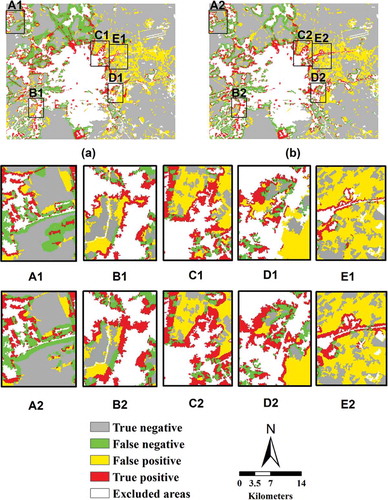
To better understand the spatial patterns contained within the simulated maps, the model’s error maps were determined by overlaying the simulated maps for 2014 on to the observed maps for 1999 and 2014 in Tehran (Figure 3) and overlaying the simulated maps for 2014 on to the observed maps for 2004 and 2014 in Isfahan (Figure 4). Consequently, the following categories were identified: (1) True positive: Changed cells correctly predicted by both the models and the reference maps, (2) True negative: Unchanged cells correctly predicted by both the models and the reference maps, (3) False positive: Cells for which the reference maps predicted a change, but for which the models predicted no change, and (4) False negative: Cells identified as unchanged by the reference map, but identified by the models as changed. As seen from Figures 3 and 4 the overall performance of the models seems similar. However, by enlarging the LTM and LTM-CA with a 7 × 7 filter size, the discrepancy between the least and most accurate models becomes evident (Figures 5 and 6).

Figure 3. Error maps for Tehran (a) LTM-CA with a 3 × 3 neighborhood size, (b) LTM-CA with a 5 × 5 neighborhood size, (c) LTM-CA with a 7 × 7 neighborhood size, (d) LTM-CA with a 9 × 9 neighborhood size, and (e) LTM with a top-down approach. The maps show the levels of agreement and disagreement between the simulated and reference maps.

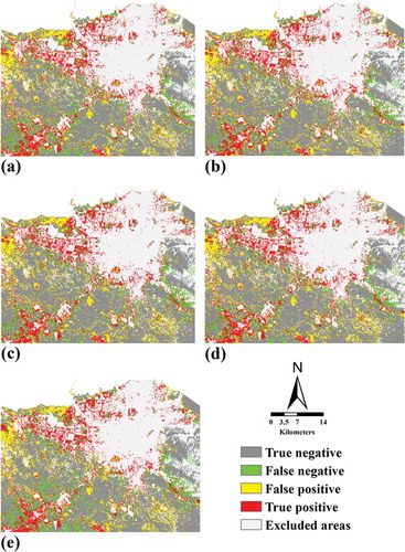
Figure 4. Error maps for Isfahan (a) LTM-CA with a 3 × 3 neighborhood size, (b) LTM-CA with a 5 × 5 neighborhood size, (c) LTM-CA with a 7 × 7 neighborhood size, (d) LTM-CA with a 9 × 9 neighborhood size, and (e) LTM with a top-down approach. The maps show the levels of agreement and disagreement between the simulated and reference maps.

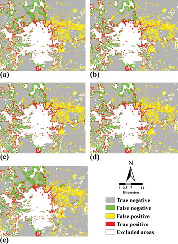
Figure 5. The difference between the LTM with a top-down approach (a, A1, B1, C1, D1, and E1) and LTM-CA with 7 × 7 neighborhood size (b, A2, B2, C2, D2, and E2) for Tehran.

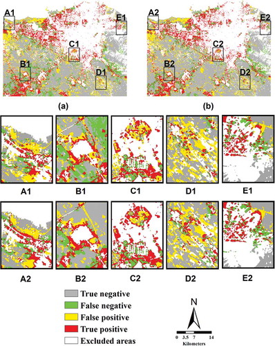
Figure 6. The difference between the LTM with a top-down approach (a, A1, B1, C1, D1, and E1) and LTM-CA with 7 × 7 neighborhood size (b, A2, B2, C2, D2, and E2) for Isfahan.

For Teheran, the results of the statistical measures (Table 3) also show that the FoM values were 40.82%, 42.72%, 43.66%, 43.72%, and 43.66%, the PA values were 57.98%, 59.87%, 60.78%, 60.84%, and 60.78%, and the OA values were 82.92%, 84.14%, 84.73%, 84.76%, and 84.73%, for the ANN (LTM), ANN-CA with a 3 × 3 neighborhood size, ANN-CA with a 5 × 5 neighborhood size, ANN-CA with a 7 × 7 neighborhood size, and ANN-CA with a 9 × 9 neighborhood size models, respectively.

Table 3. Accuracy assessment of the models indicated by the FOM, OA, and PA.

Tehran	PA	OA	FOM	Isfahan	PA	OA	FOM
LTM	57.98	82.92	40.82	LTM	38.92	70.49	24.19
LTM-CA 3 × 3	59.87	84.14	42.72	LTM-CA 3 × 3	41.56	71.77	26.26
LTM-CA 5 × 5	60.78	84.73	43.66	LTM-CA 5 × 5	42.54	72.24	27.05
LTM-CA 7 × 7	60.84	84.76	43.72	LTM-CA 7 × 7	42.69	72.31	27.16
LTM-CA 9 × 9	60.78	84.73	43.66	LTM-CA 9 × 9	42.17	72.06	26.74

For Isfahan, the FoM values were 24.19%, 26.26%, 27.05%, 27.16%, and 26.74%, the PA values were 38.92%, 41.56%, 42.54%, 42.69%, and 42.17%, and the OA values were 70.49%, 71.77%, 72.24%, 72.31%, and 72.06%, for the ANN (LTM), ANN-CA with a 3 × 3 neighborhood size, ANN-CA with a 5 × 5 neighborhood size, ANN-CA with a 7 × 7 neighborhood size, and ANN-CA with a 9 × 9 neighborhood size models, respectively.

As revealed by the statistical measures, both the LTM and the LTM-CA with varying neighborhood sizes achieved promising results, that is, they were all able to simulate at least 57% of the observed changed cells for Tehran and over 82% of the unchanged cells. For Isfahan, roughly 39% of the observed changed cells were correctly predicted and over 70% of the unchanged cells. However, the use of CA was able to improve the spatial accuracy of LTM for simulating urban growth by approximately 3% for Tehran and almost 4% for Isfahan. Even though this accuracy gain seems minor, this highlights the importance of using CA and also taking into account neighborhood effects within the LTM allocation process.

6. Conclusions

Since there is an extensive body of literature on the utility of CA in land change simulation, the focus of this paper was to evaluate the importance of a CA model in correctly allocating the cells which are going to change. The LTM was used to project urban growth in Tehran and Isfahan, using two spatial allocation strategies, namely a CA and a top-down approach.

Based on the empirical findings, it can be concluded that even though both the CA and top-down strategies were able to satisfactorily simulate urban growth, the CA model effectively improved the accuracy of the simulated land use maps. This is due to the fact that CA considers the spatial vicinity of a cell. The CA was implemented using varying neighborhood sizes, and although the CA model with a 7 × 7 neighborhood size proved to be the most accurate, the various neighborhood sizes used produced rather similar outcomes in view of the correct allocation rate.

However, this paper was limited to only two study areas, and thus implementation of the same framework is highly recommended for other cities in different geographical regions. Further, evaluating the effect of CA on the random forest, logistic regression and support vector machine is recommended, because CA has also been integrated with these techniques for the land change simulation.

Disclosure statement

No potential conflict of interest was reported by the authors.

Notes

1. One of the top 10 biggest cities in Iran located in the west of Tehran.

References

- Almeida, C. M., J. M. Gleriani, E. F. Castejon, and B. S. Soares‐Filho. 2008. “Using Neural Networks and Cellular Automata for Modelling Intra‐Urban Land‐Use Dynamics.” International Journal of Geographical Information Science 22 (9): 943–963. doi:10.1080/13658810701731168.
- Azari, M., A. Tayyebi, M. Helbich, and M. A. Reveshty. 2016. “Integrating Cellular Automata, Artificial Neural Network and Fuzzy Set Theory to Simulate Threatened Orchards: Application to Maragheh, Iran.” Giscience & Remote Sensing 53 (2): 183–205. doi: 10.1023/A:1022960300693.
- Batty, M. 2000. “Geocomputation Using Cellular Automata.” In Geocomputation, 95–126. New York: Taylor and Francis.
- Batty, M. 2007. Cities and Complexity: Understanding Cities with Cellular Automata, Agent-Based Models, and Fractals. The MIT press.
- Batty, M., Y. Xie, and Z. Sun. 1999. “Modeling Urban Dynamics through GIS-Based Cellular Automata.” Computers, Environment and Urban Systems 23 (3): 205–233. doi:10.1016/S0198-9715(99)00015-0.
- Bihamta, N., A. Soffianian., S. Fakheran., and M. Gholamalifard. 2015. “Using the SLEUTH Urban Growth Model to Simulate Future Urban Expansion of the Isfahan Metropolitan Area, Iran.” Journal of the Indian Society of Remote Sensing 43 (2): 407–414. doi:10.1007/s12524-014-0402-8.
- Blecic, I., A. Cecchini, and G. A. Trunfio. 2014. “Training Cellular Automata to Simulate Urban Dynamics: A Computational Study Based on GPGPU and Swarm Intelligence.” In Cellular Automata, 300–309. Springer International Publishing.
- Boerner, R. E., M. N. DeMers, J. W. Simpson, F. J. Artigas, A. Silva, and L. A. Berns. 1996. “Markov Models of Inertia and Dynamism on Two Contiguous Ohio Landscapes.” Geographical Analysis 28 (1): 56–66. doi:10.1111/j.1538-4632.1996.tb00921.x.
- Census Information. 2011. “Census Information, Tehran: The Statistical Centre of Iran.” http://amar.sci.org.ir/indexe.aspx.
- Clarke, K. C., and L. J. Gaydos. 1998. “Loose-Coupling a Cellular Automaton Model and GIS: Long-Term Urban Growth Prediction for San Francisco and Washington/Baltimore.” International Journal of Geographical Information Science 12 (7): 699–714. doi:10.1080/136588198241617.
- Corner, R. J., A. M. Dewan, and S. Chakma. 2014. “Monitoring and Prediction of Land-Use and Land-Cover (LULC) Change.” In Dewan, A. and Corner, R. (ed)Dhaka Megacity, 75–97. Springer Netherlands.
- Dewan, A. M., M. H. Kabir, K. Nahar, and M. Z. Rahman. 2012. “Urbanisation and Environmental Degradation in Dhaka Metropolitan Area of Bangladesh.” International Journal of Environment and Sustainable Development 11 (2): 118–147. doi:10.1504/IJESD.2012.049178.
- Dewan, A. M., and Y. Yamaguchi. 2009a. “Land Use and Land Cover Change in Greater Dhaka, Bangladesh: Using Remote Sensing to Promote Sustainable Urbanization.” Applied Geography 29 (3): 390–401. doi:10.1016/j.apgeog.2008.12.005.
- Dewan, A. M., and Y. Yamaguchi. 2009b. “Using Remote Sensing and GIS to Detect and Monitor Land Use and Land Cover Change in Dhaka Metropolitan of Bangladesh during 1960–2005.” Environmental Monitoring and Assessment 150 (1–4): 237–249. doi:10.1007/s10661-008-0226-5.
- Feng, Y., and Y. Liu. 2013. “A Heuristic Cellular Automata Approach for Modelling Urban Land-Use Change Based on Simulated Annealing.” International Journal of Geographical Information Science 27 (3): 449–466. doi:10.1080/13658816.2012.695377.
- Feng, Y., Y. Liu, X. Tong, M. Liu, and S. Deng. 2011. “Modeling Dynamic Urban Growth Using Cellular Automata and Particle Swarm Optimization Rules.” Landscape and Urban Planning 102 (3): 188–196. doi:10.1016/j.landurbplan.2011.04.004.
- Fischer, M. M. 2006. “Neural Networks: A General Framework for Non‐Linear Function Approximation.” Transactions in GIS 10 (4): 521–533. doi:10.1111/tgis.2006.10.issue-4.
- Grekousis, G., P. Manetos, and Y. N. Photis. 2013. “Modeling Urban Evolution Using Neural Networks, Fuzzy Logic and GIS: The Case of the Athens Metropolitan Area.” Cities 30: 193–203. doi:10.1016/j.cities.2012.03.006.
- Grekousis, G., and G. Mountrakis. 2015. “Sustainable Development under Population Pressure: Lessons from Developed Land Consumption in the Conterminous US.” PLoS One 10 (3): e0119675. doi:10.1371/journal.pone.0119675.
- Grekousis, G., G. Mountrakis, and M. Kavouras. 2016. “Linking Modis-Derived Forest and Cropland Land Cover 2011 Estimations to Socioeconomic and Environmental Indicators for the European Union’s 28 Countries.” Giscience & Remote Sensing 53 (1): 122–146. doi:10.1080/15481603.2015.1118977.
- Hagenauer, J., and M. Helbich. 2012. “Mining Urban Land-Use Patterns from Volunteered Geographic Information by Means of Genetic Algorithms and Artificial Neural Networks.” International Journal of Geographical Information Science 26 (6): 963–982. doi:10.1080/13658816.2011.619501.
- Kamusoko, C., and J. Gamba. 2015. “Simulating Urban Growth Using a Random Forest-Cellular Automata (RF-CA) Model.” ISPRS International Journal of Geo-Information 4 (2): 447–470. doi:10.3390/ijgi4020447.
- Lambin, E. F., H. J. Geist, and E. Lepers. 2003. “Dynamics of Land-Use and Land-Cover Change in Tropical Regions.” Annual Review of Environment and Resources 28 (1): 205–241. doi:10.1146/annurev.energy.28.050302.105459.
- Li, X., and A. G. O. Yeh. 2000. “Modelling Sustainable Urban Development by the Integration of Constrained Cellular Automata and GIS.” International Journal of Geographical Information Science 14 (2): 131–152. doi:10.1080/136588100240886.
- Li, X., and A. G. O. Yeh. 2001. “Calibration of Cellular Automata by Using Neural Networks for the Simulation of Complex Urban Systems.” Environment and Planning A 33 (8): 1445–1462. doi:10.1068/a33210.
- Li, X., and A. G. O. Yeh. 2002. “Neural-Network-Based Cellular Automata for Simulating Multiple Land Use Changes Using GIS.” International Journal of Geographical Information Science 16 (4): 323–343. doi:10.1080/13658810210137004.
- Liao, J., L. Tang, G. Shao, X. Su, D. Chen, and T. Xu. 2016. “Incorporation of Extended Neighborhood Mechanisms and Its Impact on Urban Land-Use Cellular Automata Simulations.” Environmental Modelling & Software 75: 163–175. doi:10.1016/j.envsoft.2015.10.014.
- Lin, Y.-P., H.-J. Chu, C.-F. Wu, and P. H. Verburg. 2011. “Predictive Ability of Logistic Regression, Auto-Logistic Regression and Neural Network Models in Empirical Land-Use Change Modeling–A Case Study.” International Journal of Geographical Information Science 25 (1): 65–87. doi:10.1080/13658811003752332.
- Liu, Y. 2008. Modelling Urban Development with Geographical Information Systems and Cellular Automata. Boca Raton: CRC Press.
- Madanipour, A. 2006. “Urban Planning and Development in Tehran.” Cities 23 (6): 433–438. doi:10.1016/j.cities.2006.08.002.
- Mitsova, D., W. Shuster, and X. Wang. 2011. “A Cellular Automata Model of Land Cover Change to Integrate Urban Growth with Open Space Conservation.” Landscape and Urban Planning 99 (2): 141–153. doi:10.1016/j.landurbplan.2010.10.001.
- Mozumder, C., and N. K. Tripathi. 2014. “Geospatial Scenario Based Modelling of Urban and Agricultural Intrusions in Ramsar Wetland Deepor Beel in Northeast India Using a Multi-Layer Perceptron Neural Network.” International Journal of Applied Earth Observation and Geoinformation 32: 92–104. doi:10.1016/j.jag.2014.03.002.
- Newman, G., J. Lee, and P. Berke. 2016. “Using the Land Transformation Model to Forecast Vacant Land.” Journal of Land Use Science 11(4): 450–475.
- Olmedo, M. T. C., R. G. Pontius, M. Paegelow, and J.-F. Mas. 2015. “Comparison of Simulation Models in Terms of Quantity and Allocation of Land Change.” Environmental Modelling & Software 69: 214–221. doi:10.1016/j.envsoft.2015.03.003.
- Ozturk, D. 2015. “Urban Growth Simulation of Atakum (Samsun, Turkey) Using Cellular Automata-Markov Chain and Multi-Layer Perceptron-Markov Chain Models.” Remote Sensing 7 (5): 5918–5950. doi:10.3390/rs70505918.
- Pijanowski, B. C., D. G. Brown, B. A. Shellito, and G. A. Manik. 2002. “Using Neural Networks and GIS to Forecast Land Use Changes: A Land Transformation Model.” Computers, Environment and Urban Systems 26 (6): 553–575. doi:10.1016/S0198-9715(01)00015-1.
- Pijanowski, B. C., S. H. Gage, D. T. Long, and W. C. Cooper. 2000. “A Land Transformation Model: Integrating Policy, Socioeconomics and Environmental Drivers Using A Geographic Information System.” In Landscape Ecology: A Top-Down Approach, edited by L. Harris and J. Sanderson. Boca Raton: Lewis Publishers.
- Pijanowski, B. C., S. Pithadia, B. A. Shellito, and K. Alexandridis. 2005. “Calibrating a Neural Network‐Based Urban Change Model for Two Metropolitan Areas of the Upper Midwest of the United States.” International Journal of Geographical Information Science 19 (2): 197–215. doi:10.1080/13658810410001713416.
- Pijanowski, B. C., A. Tayyebi, M. R. Delavar, and M. J. Yazdanpanah. 2009. “Urban Expansion Simulation Using Geospatial Information System and Artificial Neural Networks.” International Journal of Environmental Research 3 (4): 493-502.
- Pontius, G. R., and J. Malanson. 2005. “Comparison of the Structure and Accuracy of Two Land Change Models.” International Journal of Geographical Information Science 19 (2): 243–265. doi:10.1080/13658810410001713434.
- Pontius, R. Jr, G. W. Boersma, J.-C. Castella, K. Clarke, T. De Nijs, C. Dietzel, Z. Duan, et al. 2008. “Comparing the Input, Output, and Validation Maps for Several Models of Land Change.” The Annals of Regional Science 42 (1): 11–37. doi:10.1007/s00168-007-0138-2.
- Serneels, S., and E. F. Lambin. 2001. “Proximate Causes of Land-Use Change in Narok District, Kenya: A Spatial Statistical Model.” Agriculture, Ecosystems & Environment 85 (1–3): 65–81. doi:10.1016/S0167-8809(01)00188-8.
- Shafizadeh-Moghadam, H., J. Hagenauer, M. Farajzadeh, and M. Helbich. 2015. “Performance Analysis of Radial Basis Function Networks and Multi-Layer Perceptron Networks in Modeling Urban Change: A Case Study.” International Journal of Geographical Information Science 29 (4): 606–623. doi:10.1080/13658816.2014.993989.
- Shafizadeh-Moghadam, H., and M. Helbich. 2015. “Spatiotemporal Variability of Urban Growth Factors: A Global and Local Perspective on the Megacity of Mumbai.” International Journal of Applied Earth Observation and Geoinformation 35: 187–198. doi:10.1016/j.jag.2014.08.013.
- Soffianian, A., M. A. Nadoushan, L. Yaghmaei, and S. Falahatkar. 2010. “Mapping and Analyzing Urban Expansion Using Remotely Sensed Imagery in Isfahan, Iran.” World Applied Sciences Journal 9 (12): 1370–1378.
- Taubenböck, H., T. Esch, A. Felbier, M. Wiesner, A. Roth, and S. Dech. 2012. “Monitoring Urbanization in Mega Cities from Space.” Remote Sensing of Environment 117: 162–176. doi:10.1016/j.rse.2011.09.015.
- Tayyebi, A., and B. C. Pijanowski. 2014. “Modeling Multiple Land Use Changes Using ANN, CART and MARS: Comparing Tradeoffs in Goodness of Fit and Explanatory Power of Data Mining Tools.” International Journal of Applied Earth Observation and Geoinformation 28: 102–116. doi:10.1016/j.jag.2013.11.008.
- Tayyebi, A., A. H. Tayyebi, J. J. Arsanjani, H. Shagizadeh-Moghadam, and H. Omrani. 2016. “Fsaua: A Framework For Sensitivity Analysis And Uncertainty Assessment In Historical And Forecasted Land Use Maps.” Environmental Modelling & Software 84: 70-84. doi:10.1016/j.envsoft.2016.06.018.
- Thapa, R. B., and Y. Murayama. 2011. “Urban Growth Modeling of Kathmandu Metropolitan Region, Nepal.” Computers, Environment and Urban Systems 35 (1): 25–34. doi:10.1016/j.compenvurbsys.2010.07.005.
- Tobler, W. R. 1970. “A Computer Movie Simulating Urban Growth in the Detroit Region.” Economic Geography 46: 234–240. doi:10.2307/143141.
- Veldkamp, A., and E. F. Lambin. 2001. “Predicting Land-Use Change.” Agriculture, Ecosystems & Environment 85 (1–3): 1–6. doi:10.1016/S0167-8809(01)00199-2.
- Verburg, P. H., and K. P. Overmars. 2009. “Combining Top-Down and Bottom-Up Dynamics in Land Use Modeling: Exploring the Future of Abandoned Farmlands in Europe with the Dyna-CLUE Model.” Landscape Ecology 24 (9): 1167–1181. doi:10.1007/s10980-009-9355-7.
- Verburg, P. H., W. Soepboer, A. Veldkamp, R. Limpiada, V. Espaldon, and S. S. Mastura. 2002. “Modeling the Spatial Dynamics of Regional Land Use: The CLUE-S Model.” Environmental Management 30 (3): 391–405. doi:10.1007/s00267-002-2630-x.
- Verstegen, J. A., D. Karssenberg, F. Van der Hilst, and A. P. Faaij. 2014. “Identifying a Land Use Change Cellular Automaton by Bayesian Data Assimilation.” Environmental Modelling & Software 53: 121–136. doi:10.1016/j.envsoft.2013.11.009.
- White, R., and G. Engelen. 1993. “Cellular Automata and Fractal Urban Form: A Cellular Modelling Approach to the Evolution of Urban Land-Use Patterns.” Environment and Planning A 25 (8): 1175–1199. doi:10.1068/a251175.
- Wu, F. 2002. “Calibration of Stochastic Cellular Automata: The Application to Rural-Urban Land Conversions.” International Journal of Geographical Information Science 16 (8): 795–818. doi:10.1080/13658810210157769.
- Wu, F., and C. J. Webster. 1998. “Simulation of Land Development through the Integration of Cellular Automata and Multicriteria Evaluation.” Environment and Planning B: Planning and Design 25 (1): 103–126. doi:10.1068/b250103.
- Yang, Q., X. Li, and X. Shi. 2008. “Cellular Automata for Simulating Land Use Changes Based on Support Vector Machines.” Computers & Geosciences 34 (6): 592–602. doi:10.1016/j.cageo.2007.08.003.
- Yeh, A. G. O., and X. Li. 2002. “A Cellular Automata Model to Simulate Development Density for Urban Planning.” Environment and Planning B: Planning and Design 29 (3): 431–450. doi:10.1068/b1288.