CO₂ concentration and its spatiotemporal variation in the troposphere using multi-sensor satellite data, carbon tracker, and aircraft observations

Abstract

Satellite-based atmospheric CO₂ observations have provided a great opportunity to improve our understanding of the global carbon cycle. However, thermal infrared (TIR)-based satellite observations, which are useful for the investigation of vertical distribution and the transport of CO₂, have not yet been studied as much as the column amount products derived from shortwave infrared data. In this study, TIR-based satellite CO₂ products – from Atmospheric Infrared Sounder, Tropospheric Emission Spectrometer (TES), and Thermal And Near infrared Sensor for carbon Observation – and carbon tracker mole fraction data were compared with in situ Comprehensive Observation Network for Trace gases by AIrLiner (CONTRAIL) data for different locations. The TES CO₂ product showed the best agreement with CONTRAIL CO₂ data resulting in R² ~ 0.87 and root-mean-square error ~0.9. The vertical distribution of CO₂ derived by TES strongly depends on the geophysical characteristics of an area. Two different climate regions (i.e., southeastern Japan and southeastern Australia) were examined in terms of the vertical distribution and transport of CO₂. Results show that while vertical distribution of CO₂ around southeastern Japan was mainly controlled by horizontal and vertical winds, horizontal wind might be a major factor to control the CO₂ transport around southeastern Australia. In addition, the vertical transport of CO₂ also varies by region, which is mainly controlled by anthropogenic CO₂, and horizontal and omega winds. This study improves our understanding of vertical distribution and the transport of CO₂, both of which vary by region, using TIR-based satellite CO₂ observations and meteorological variables.

Keywords:

• atmospheric CO₂
• TES
• CONTRAIL
• vertical distribution
• CO₂ transport

1. Introduction

Carbon dioxide (CO₂) is the most important anthropogenic greenhouse gas. An increase in the amount of CO₂ in the atmosphere forces the Earth’s radiation budget by absorbing radiation from energy and therefore accelerates the greenhouse effect (Forster et al. 2007). The major causes of increased atmospheric CO₂ concentration include the combustion of fossil fuels, cement production, and land-use change (Keeling, Piper, and Heimann 2013). The seasonal cycle of atmospheric CO₂ has been investigated using in situ field measurements since the mid-1950s (Keeling, Chin, and Whorf 1996) and the network of field measurements has been expanded throughout the world (Baldocchi et al. 2001). However, field measurements are not spatially continuous and one cannot measure data easily over inaccessible regions such as the Amazon, which results in large uncertainty about the spatial distribution of CO₂ concentration (Gurney et al. 2008). In this context, spaceborne remote sensing is very appealing because of its ability to collect data over vast areas (Chevallier, Bréon, and Rayner 2007).

There are three satellite-based techniques for the estimation of atmospheric CO₂ concentration. One approach is the differential absorption technique, which uses CO₂ absorption wavelengths in the shortwave infrared region (SWIR; ~1.6–2.0 m) (Bréon and Ciais 2010). For example, Thermal And Near infrared Sensor for carbon Observation (TANSO) onboard the Greenhouse gases Observing SATellite (GOSAT) uses an inverse method, which is an iterative retrieval based on Bayesian optimal estimation. It corrects simulated spectral radiance data from measured spectral radiance (Rodgers 2000). While the wavelengths are sensitive to CO₂ and can be used to distinguish CO₂ from other trace gases, the approach requires a clear sky with sunlight above the horizon. The other approach is to use thermal infrared (TIR; >4 m) remote sensing to quantify the vertical distribution of CO₂ concentration based on the fact that radiance emitted by CO₂ gases in the atmosphere is a function of temperature (Bréon and Ciais 2010). The SWIR-based CO₂ estimation shows better sensitivity to the surface than TIR-based CO₂ estimation because SWIR gives approximately constant sensitivity through the troposphere. Solar occultation is another method to retrieve a CO₂ profile, which provides better profile information at about 5 km (Patra et al. 2008; Foucher et al. 2011; Sioris et al. 2014). Additionally, Active Sensing of CO₂ emissions over Nights, Days, and Seasons can also measure atmospheric CO₂ in a unique way by using an active laser sensor (Numata et al. 2011).

Atmospheric CO₂ observation using satellite sensors started in 2002 with SCanning Imaging Absorption spectroMeter for Atmospheric CartograpHY (SCIAMACHY) onboard Envisat by the European Space Agency. Due to the large footprint of SCIAMACHY, a considerable amount of observations was spoiled by clouds, which can influence the accuracy of the SCIAMACHY observations (Ceos 2014). Atmospheric Infrared Sounder (AIRS) onboard Aqua launched by the National Aeronautics Space Administration (NASA) had been mainly used to measure water vapor and temperature profiles in the atmosphere (Ceos 2014). Chédin et al. (2003) and Engelen and Stephens (2004) showed the potential of AIRS for retrieving vertical concentrations of atmospheric CO₂. AIRS has been used to monitor atmospheric CO₂ in relation to meteorological and climatic phenomena (Chédin et al. 2003; Jiang et al. 2012). The Tropospheric Emission Spectrometer (TES) on Aura is also used to produce CO₂ concentration products, which were evaluated with airborne measurements, models (i.e., Carbon Tracker), and AIRS products (Kulawik et al., 2010; Kulawik et al. 2013). Inverse modeling, based on TES CO₂ observations, was used to estimate CO₂ surface fluxes (Nassar et al. 2011). The Infrared Atmospheric Sounding Interferometer (IASI) onboard the Meteorological Operational satellite program (MetOp-A) has similar spectral characteristics to TES. IASI observes atmospheric CO₂ only in the tropical belt (i.e., 20–20) (Crevoisier et al. 2009). The TANSO onboard the GOSAT was the first project developed to measure greenhouse gases such as CO₂ and CH₄ with SWIR and TIR bands. TANSO has been used to develop and improve the retrieval algorithms of CO₂ column abundance (Yoshida, Kikuchi, and Yokota 2012; Crisp et al. 2012; O’Dell et al. 2012; Yoshida et al. 2013). Orbiting Carbon Observatory-2, NASA’s first dedicated CO₂ mission, was launched in July 2014 (Crisp et al. 2004; Miller et al. 2007) and provides Level 1 geolocated spectra and Level 2 XCO₂ products.

While many studies on the estimation of CO₂ column abundance have been carried out based on SWIR and its retrieval algorithms, the vertical distribution of CO₂ concentration based on TIR has not been fully investigated. There are several reasons why the quantification of vertical distribution of CO₂ is important. First, the vertical profile of CO₂ is essential to calculate CO₂ fluxes at the small scale using a boundary-layer budget method. Second, the vertical distribution of CO₂ helps us to understand the vertical transport of CO₂ in the troposphere. There have been efforts to study and understand the vertical distribution and transport of CO₂ using satellite data. Crevoisier et al. (2009) investigated the vertical transport of CO₂ based on the fact that the CO₂ seasonal cycles between IASI and Comprehensive Observation Network for Trace gases by AIrLiner (CONTRAIL) have a 1-month time lag. While Crevoisier et al. (2009) did not analyze drivers to transport CO₂, Kumar, Revadekar, and Tiwari (2014) proposed that vertical wind motion via convection might transport CO₂ from the surface to the mid-troposphere over India. In addition to satellite remote-sensing data, aircraft and tethered balloon-derived data were used to analyze the vertical distribution of CO₂ and its characteristics (Li et al. 2014; Sawa, Machida, and Matsueda 2012; Sweeney et al. 2015). However, the vertical distribution of CO₂ varies by region because of different environmental characteristics, such as vegetation phenology, land composition, distribution of geographical features, atmospheric conditions, wind patterns, and anthropogenic emissions.

This study extends our preliminary research in Lee, Im, and Lee (2015), which compared multiple CO₂ satellite products from AIRS, TES, and TANSO with aircraft observations (i.e., CONTRAIL). This present study compares the TIR-based CO₂ products and carbon tracker data with CONTRAIL data in more detail over four study sites. We further investigated mechanisms of vertical distribution and transport of CO₂ using the satellite product that showed the best agreement with the in situ CONTRAIL and the carbon tracker data. Two regions with different environmental and climatic characteristics were selected for this purpose, including southeastern Japan and southeastern Australia.

2. Materials and methods

2.1. Satellite data

AIRS onboard Aqua collects data across 2378 channels between 3.7 and 15.4  with a 13.5 km field of view at nadir (Aumann and Pagano, 2003). In order to eliminate the effects of clouds, it is combined with the Advanced Microwave Sounding Unit (AMSU) and produces temperature profiles as well as the concentrations of trace gases, including CO₂, CO, SO₂, and CH₄ (Pagano, Chahine, and Olsen 2011). It is known that the accuracy of AIRS CO₂ is around 1–2 ppm between 30 and 80 when compared to aircraft measurements and Fourier Transform Interferometers (Chahine et al. 2008). AIRS Version 5 Level 2 CO₂ data (ftp://airsl2.gesdisc.eosdis.nasa.gov/ftp/data/s4pa/Aqua_AIRS_Level2/AIRX2STC.005ftp://airsl2.gesdisc.eosdis.nasa.gov/ftp/data/s4pa/Aqua_AIRS_Level2/AIRX2STC.005) were used in this study. This product assumes a global average linear time-variable CO₂ climatology throughout the atmosphere (Olsen 2009). AIRS data until 28 February 2012 were used due to the degradation of AMSU for consistent comparison.

TES on AURA collects data at very high spectral resolution with nadir measurements of TIR emission (3.2–15.4 ). It was launched on 15 July 2004 at an altitude of approximately 686 km with a coverage between 40 and 40. The peak sensitivity of TES was reported near 511 hPa atmospheric pressure level (Nassar et al. 2011). The number of TES CO₂ observations was largest in 2007 and 2008. However, it has consistently decreased since 2009. In order for comparisons with airborne observations, this study used the TES CO₂ product between 2006 and 2012. The data version is TES L2 CO₂ v7 lite product, which provides the concentration values at 14 atmospheric pressure layers from the ground to the altitude of 64 km (http://avdc.gsfc.nasa.gov/index.php?site=635564035&id=10&go=list&path=/CO2).

GOSAT, launched on 23 January 2009, is the first satellite dedicated to the retrieval of the amount of greenhouse gases such as CO₂ and CH₄ in the atmosphere (Kuze et al. 2009). TANSO is the main sensor of GOSAT. It has two main instruments: the Fourier Transform Spectrometer (FTS) and the Cloud and Aerosol Imager. TANSO-FTS has three narrow SWIR bands (i.e., 0.76, 1.6, and 2.0 ) and a wide thermal band (5.5–14.3  (Yokota et al. 2009). While the SWIR bands are used to retrieve CO₂ column concentration, the TIR band is used to retrieve the vertical profile of CO₂ concentration (Imasu et al. 2008). In this study, TANSO-FTS TIR level 2 v00.01 data was used (http://data.gosat.nies.go.jp/GosatUserInterfaceGateway/guig/GuigPage/open.do), which was available for only 9 months from March to November 2010 with three altitudes (i.e., 3, 5.5, and 9.1 km).

2.2. CONTRAIL

The CONTRAIL project was developed to automatically measure atmospheric CO₂ concentrations using the Continuous CO₂ Measuring Equipment (CME) and Automatic Air Sampling Equipment that are installed in commercial aircraft from 1993 to the present (Machida et al. 2008). The CME CO₂ concentration data were used in this study. The CME observation device records the CO₂ concentrations every 10 s when an aircraft ascends or descends, with an approximately 100 m interval in vertical (Sawa, Machida, and Matsueda 2012). The CO₂ data were obtained from Japan Airlines’ (JAL) regular flight at the airports of major cities such as Narita and Nagoya in Japan, Bangkok in Thailand, and Paris in France in the Northern Hemisphere and Sydney in Australia in the Southern Hemisphere.

2.3. Ancillary data

To estimate the horizontal and vertical transport of CO₂, this study used the four-dimensional wind data from the National Centers for Environmental Prediction (NCEP) Department of Energy Reanalysis 2 (Kanamitsu et al. 2002), which was derived through a data assimilation technique using various in situ and satellite-based meteorological observations. The temporal coverage of NCEP R2 is from January 1979 to June 2015 and the spatial coverage is global with 2.5 grid spacing. Monthly-mean vertical (a.k.a. omega velocity in Pa s⁻¹) and horizontal winds (zonal U- and meridional V-wind) from NCEP R2 between 2006 and 2011 were downloaded from the data archive (http://www.esrl.noaa.gov/psd/data/gridded/data.ncep.reanalysis2.pressure.html#references).

Carbon tracker is the leading edge data assimilation system of CO₂ based on dry-air mole fraction observations (Peters et al. 2007). The assimilation system estimates atmospheric CO₂ mole fractions using global CO₂ surface exchange models and an atmospheric transport model derived by meteorological fields from the European Centre for Medium-Range Weather Forecasts atmospheric reanalysis. Carbon tracker 2013B mole fraction data was used from 2006 to 2011 to investigate horizontal CO₂ transport. Monthly Normalized Difference Vegetation Index (NDVI) and Net Primary Productivity (NPP) derived by Moderate Resolution Imaging Spectroradiometer from NASA Earth Observations (NEO) were used in this study. Since NDVI is a key parameter documenting vegetation phenology (Ding et al., 2016; Kim and Yeom, 2015; Yagci, Di, and Deng 2015; Zhang et al. 2017), it is useful to investigate the relationship between vegetation activity and atmospheric CO2.

2.4. Study area

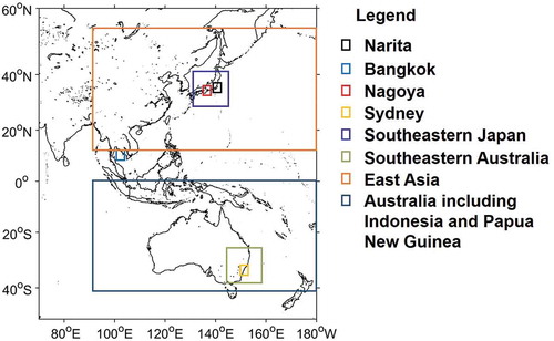
The study sites are given in Table 1 and Figure 1. Multiple regions were chosen to investigate CO₂ concentrations. Four local sites near the Narita, Bangkok, and Nagoya airports in the Northern Hemisphere, and Sydney airport in the Southern Hemisphere were chosen to compare TIR-derived satellite products with CONTRAIL data. The vertical variation of CO₂ was investigated over larger areas including southeastern Japan and southeastern Australia. East Asia and Australia, including Indonesia and Papua New Guinea, were chosen to examine the transportation of CO₂ on a continental scale.

Table 1. Study sites investigated in this research.

Location	Latitude ()	Longitude ()
Narita	35N–37N	140E–142E
Bangkok	13N–15N	100E–102E
Nagoya	34N–36N	136E–138E
Sydney	33S–35S	150E–152E
Southeastern Japan	31N–41N	136E–146E
Southeastern Australia	29–39	145E–155E
East Asia	15N–55N	90E–180E
Australia including Indonesia and Papua New Guinea	0–40	90E–180E

Figure 1. Geographical locations and spatial extent of the study sites used in this research: from Narita to Australia including Indonesia and Papua New Guinea correspond to Table 1.

2.5. A comparison between TIR-based sensors, carbon tracker, and CONTRAIL

CO₂ products from TIR-based sensors have limited spatiotemporal coincidence with the airborne CONTRAIL data. Thus, a 2 × 2 grid box for each CONTRAIL sample location was used to extract TIR-based CO₂ samples for comparison with the airborne data (Figure 1). In addition, a vertical buffer (i.e., was needed because it is hard to compare satellite-derived data with airborne observations at the exact same altitude. When both the satellite and airborne data were available for the same day regardless of time within the 500 m vertical buffer in a 2 × 2 grid box, the data pair was used for the comparison. The temporal difference for coincidences may increase the uncertainty for the comparison, which is a major limitation. However, when we used the time difference less than 1 or 2 h, the number of pairs was dramatically reduced, which made it difficult to examine the statistical significance of the relationship. In addition, carbon tracker data was provided daily; it is considered that the temporal difference for the coincidences can be negligible when compared to the carbon tracker data. The averaged time difference between CONTRAIL and TIR-based CO₂ samples was about 6 h. The number of the pairs by sensor is summarized in Table 2. Four airport sites (Narita, Bangkok, Nagoya, and Sydney) were selected for the comparison between TES and CONTRAIL since there were sufficient samples. On the other hand, the comparisons between CONTRAIL and the data from the other sensors (i.e., AIRS and TANSO) were conducted only at Narita due to the limited number of samples. When more than one CONTRAIL sample was located in a grid of the daily carbon tracker data, they were averaged.

Table 2. The number of pairs by sensor at each location of CONTRAIL observations.

Sensor	Location	The number of pairs
TES	Narita	229
TES	Bangkok	97
TES	Nagoya	70
TES	Sydney	55
AIRS	Narita	56
TANSO	Narita	25

2.6. Averaging kernels

The averaging kernel represents atmospheric physical states, such as surface and atmospheric molecular scattering, for each satellite observation point (Emmons et al. 2004; Figure 2). Since the airborne data did not contain regular pressure grids, it should be interpolated to a regular grid (Nassar et al. 2008; Kulawik et al., 2010). The A_TES, TES averaging kernel and a priori constraint vector X_prior were considered as the TES operator. The X_{airborneTESop} was produced by applying TES averaging kernel, considering the TES sensitivity and vertical resolution (Nassar et al. 2008; Kulawik et al., 2010).

(1)

Figure 2. Examples of averaging kernels for TES CO₂ lite product version 7 over East Asia (Latitude: 15N–55N, longitude: 90E–180E).

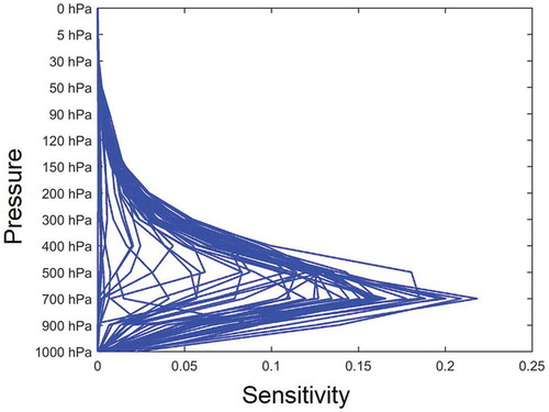
The averaging kernel of TES was applied to airborne CONTRAIL data to remove the residual between them. The sensitivity of TES is the highest around 500–700 hPa. It should be noted that the averaging kernel of AIRS was not used to keep the sensitivity of CO₂ measurements by altitude (Maddy et al. 2008). In addition, since TANSO-FTS TIR level 2 v00.01 data does not provide parameters associated with an averaging kernel, the averaging kernel was not applied to TANSO data.

3. Results and discussion

3.1. Comparison of TIR-based CO₂ and carbon tracker CO₂ concentrations with CONTRAIL data

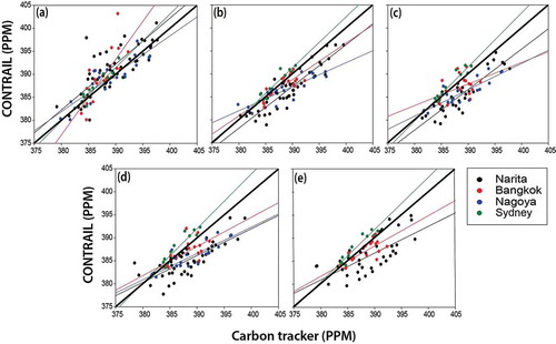
CO₂ concentrations derived from TIR-based sensors (i.e., TES, TANSO, and AIRS) during 2006–2011 were validated with CONTRAIL data (Figures 3 and 4). TES-derived CO₂ concentrations were estimated somewhat lower than CONTRAIL at 910 hPa in most sites except Sydney (i.e., the black dots in Figure 3), which implies that the TES product might not effectively capture CO₂ emitted from airplanes or other man-made sources from the ground. In addition, there is a significant diurnal cycle of CO₂ concentrations near the ground surface as observed from CONTRAIL, and the nighttime increase of CO₂ through respiration by vegetation may not be correctly represented in TES near the ground. Statistics of R² and the root-mean-square error (RMSE), and bias between TES and CONTRAIL are summarized in Table 3. The difference between TES-derived CO₂ and CONTRAIL data becomes smallest in the mid-troposphere, resulting in R² ~ 0.98, RMSE ~ 1.24 ppm, and bias ~ 0.4 ppm at 505 hPa in Narita, and R² ~ 0.93, RMSE ~ 0.92 ppm, and bias ~ −0.03 at 380 hPa in Bangkok (Figure 3 and Table 3). Sydney resulted in relatively higher R² values than the other sites, as the number of samples was small and the samples were clustered into two groups of low and high concentrations. As TES is not optimized for carbon cycle research, it has low accuracy for CO₂ concentrations near the surface (Nassar et al. 2011).

Table 3. Statistics (i.e., R² and RMSE) of the relationship between TES CO₂ product and CO₂ concentrations measured by CONTRAIL. No data available at 280 hPa in Nagoya.

Elevation (hPa)		Narita	Bangkok	Nagoya	Sydney
910	R^2	0.56	0.45	0.77	0.81
	RMSE (ppm)	5.5	4.0	3.26	2.72
	Bias (ppm)	−3.92	2.07	2.16	−1.84
675	R^2	0.95	0.9	0.95	0.90
	RMSE (ppm)	1.29	0.85	1.27	1.63
	Bias(ppm)	0.67	0.04	0.59	−1.47
505	R^2	0.98	0.91	0.94	0.91
	RMSE (ppm)	1.23	0.77	1.38	1.62
	Bias(ppm)	0.4	0.1	0.63	−1.45
380	R^2	0.94	0.93	0.92	0.84
	RMSE (ppm)	1.03	0.62	0.66	1.37
	Bias(ppm)	0.43	−0.03	0.14	−1.0
280	R^2	0.88	0.87		0.87
	RMSE (ppm)	1.15	1.02		1.36
	Bias(ppm)	0.24	−0.02		−1.1

Figure 3. Comparison between TES and CONTRAIL at different elevations: (a) 910, (b) 675, (c) 505, (d) 380, and (e) 280 hPa.

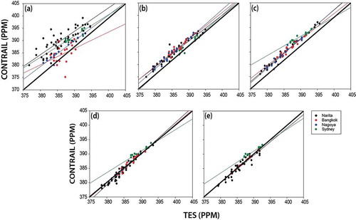
Figure 4. Comparison of TANSO-derived CO₂ and AIRS-derived CO₂ with CONTRAIL for Narita.

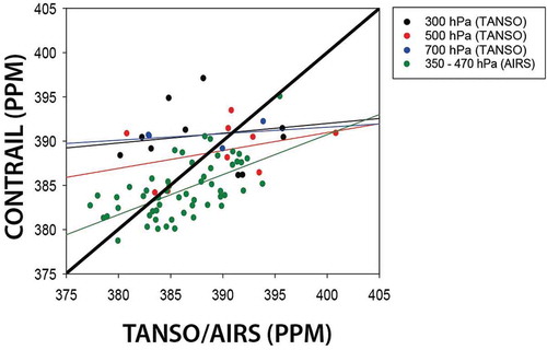
While it is known that TANSO–SWIR-derived CO₂ column concentrations have a generally good agreement with aircraft observations (Maddy et al. 2008), TANSO–TIR-derived CO₂ concentrations produced a relatively poor relationship with CONTRAIL data (Figure 4), with much lower R² and higher RMSE values at all three altitudes (Table 4), when compared with TES data. The small number of samples would be one of the reasons for such a low correlation. More samples of CO₂ measured by TANSO could improve R², RMSE, and bias. It should be noted that TANSO-derived CO₂ concentrations have not been provided since 14 July 2014.

Table 4. Statistics (i.e., R² and RMSE) of the relationship between TANSO/AIRS CO₂ products and CO₂ concentrations measured by CONTRAIL at Narita.

TANSO and CONTRAIL
Elevation (hPa)		Narita
700	R^2	0.53
	RMSE(ppm)	4.35
	Bias(ppm)	−0.29
500	R^2	0.45
	RMSE(ppm)	3.2
	Bias(ppm)	0.9
300	R^2	0.33
	RMSE(ppm)	5.6
	Bias(ppm)	−4.13
AIRS and CONTRAIL
350–470	R^2	0.5
	RMSE(ppm)	2.99
	Bias(ppm)	1.67

The peak sensitivity of AIRS-derived CO₂ varies by latitude, in which it is found at altitudes from 6 to 8 km in the mid-latitudes (i.e., 25–60 and 25–60 N) (Inoue et al. 2013). For the comparison with AIRS-derived concentrations, the CONTRAIL data was averaged for the altitudes between 6 and 8 km in Narita. AIRS-derived CO₂ produced R² ~ 0.5 and RMSE ~ 2.99 ppm in the upper troposphere at 250 hPa (Table 4). It should be noted that an averaging kernel was not used to keep the sensitivity of CO₂ measurements by altitude (Inoue et al. 2013). Maddy et al. (2008) used National Oceanic and Atmospheric Administration Earth System Research Laboratory/Global Monitoring Division aircraft flask measurements to compare AIRS CO₂ product around North America, resulting in R² ~ 0.58 and RMSE ~ 2.05 ppm. While AIRS CO₂ concentrations in the present study are generally higher than the AIRS data used in Maddy et al. (2008), both are higher than CONTRAIL data tending to overestimate CO₂ concentrations.

Although the carbon tracker has a very coarse spatial resolution, the agreement between carbon tracker CO₂ and CONTRAIL CO₂ is moderate because CO₂ is a well-mixed gas (Figure 4). The carbon tracker CO₂ near the surface (i.e., 910 hPa) better matched the CONTRAIL data when compared with TES CO₂ (Figure 5 and Table 5). The carbon tracker mole fraction data were used to show the vertical distribution of CO₂ concentrations in the Sections 3.2 and 3.3.

Table 5. Statistics (i.e., R² and RMSE) of the relationship between carbon tracker CO₂ and CO₂ concentrations measured by CONTRAIL. No data available at 280 hPa in S3.

Elevation (hPa)		Narita	Bangkok	Nagoya	Sydney
910	R^2	0.48	0.62	0.76	0.87
	RMSE (ppm)	5.28	4.08	2.37	1.47
675	R^2	0.83	0.68	0.76	0.89
	RMSE (ppm)	3.27	1.67	3.37	1.4
505	R^2	0.79	0.22	0.75	1.91
	RMSE (ppm)	3.76	2.8	3.62	1.34
380	R^2	0.57	0.47	0.66	1.88
	RMSE (ppm)	4.2	2.25	4.46	1.82
280	R^2	0.48	0.58		0.89
	RMSE (ppm)	4.4	1.97		1.65

Figure 5. Comparison between carbon tracker and CONTRAIL at different elevations: (a) 910, (b) 675, (c) 505, (d) 380, and (e) 280 hPa.

3.2. Spatiotemporal analysis of TES and carbon tracker CO₂

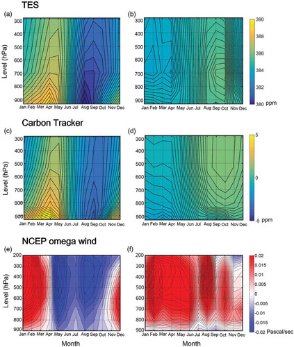
Since TES produced the best agreement with CONTRAIL data for the four local sites, TES-derived CO₂ was further investigated on the spatiotemporal domain. Figure 6(a,b) shows the seasonal and vertical variations of CO₂ at two different sites (i.e., southeastern Japan and southeastern Australia in Figure 1), which are obtained for five vertical layers at 910, 675, 505, 380, and 280 hPa from TES and averaged for 2006–2011. The two sites exhibit quite distinctive seasonal and vertical variations of CO₂. While southeastern Japan shows a strong seasonal cycle (Figure 6(a)) (Gurney et al. 2002; Tian et al. 2003; Shim, Lee, and Wang 2013), southeastern Australia shows a relatively weak seasonal cycle (Figure 6(b)). The carbon tracker CO₂ anomaly was calculated during 2006–2011 (Figure 6(c,d)). While there is a slight difference between TES and carbon-tracker-derived CO₂ concentrations for the CO₂ minimum month, the overall vertical distribution of carbon tracker CO₂ is very similar to that of TES CO₂. Since the CO₂ concentration at southeastern Japan is significantly influenced by the seasonal variations of the terrestrial biosphere in the Northern Hemisphere as well as by many nearby anthropogenic sources, it shows stronger seasonal variations, with the maximum in April (Figure 6). It is the lowest in August because of the vegetation uptake during summer (Harazono et al. 2003; Stephens et al. 2007; Garbulsky et al. 2008). Myneni et al. (2001) suggested that the Russian tundra plays a meaningful role in absorbing the atmospheric CO₂. Meanwhile, the seasonal variation of CO₂ at southeastern Australia is much smaller, presumably due to less natural and anthropogenic CO₂ sources in the Southern Hemisphere. The relationship between seasonal variations of CO₂ and omega wind is analyzed in the next section.

Figure 6. Vertical TES and carbon tracker monthly CO₂ variations and omega wind (vertical pressure velocity) averaged during 2006–2011 at southeastern Japan (a, c, e) and southeastern Australia (b, d, f).

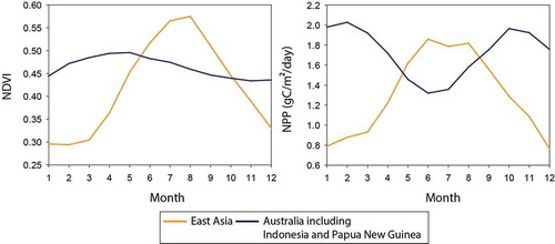
Figure 7 shows the monthly NDVI and NPP averaged for 2006–2011 in two larger regions (i.e., East Asia and Australia including Indonesia and Papua New Guinea) to examine the influence of vegetation activities. It is known that NDVI is often saturated over dense vegetation such as tropical forests (Forkel et al. 2016), which makes NPP more sensitive to the phenology of vegetation than NDVI over dense vegetation especially at Australia including Indonesia and Papua New Guinea. The amplitude of the seasonal cycle of NDVI and NPP at East Asia is larger than that of NDVI and NPP at Australia including Indonesia and Papua New Guinea. The seasonal variation of CO₂ is closely related to the phenological cycle of vegetation (Mutanga and Skidmore 2004). Especially, vegetation activities have a great impact on the dynamics of the carbon cycle in the Northern Hemisphere (Mutanga and Skidmore 2004). A large variation of NDVI and NPP at East Asia may explain the large fluctuation of CO₂ concentrations at southeastern Japan (Figure 7) (Shim, Lee, and Wang 2013; Fan et al. 1998; Angert et al. 2005). The seasonal cycle of NDVI and NPP at Australia including Indonesia and Papua New Guinea (darker (blue) line in Figure 7) is totally out of phase with that at East Asia, with a smaller amplitude. The difference in the biomass between the Northern and the Southern Hemisphere and the saturation effect of NDVI should explain the difference in the amplitude of the NDVI seasonal cycle between the two sites.

Figure 7. Monthly NDVI and NPP averaged during 2006–2011 provided by NASA Earth Observation (NEO) over two regions (i.e., East Asia and Australia including Indonesia and Papua New Guinea). For full color versions of the figures in this paper, please see the online version.

3.3. Vertical and horizontal transport of CO₂

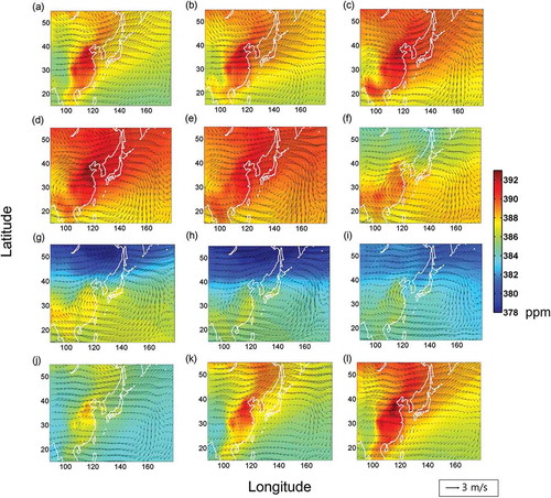
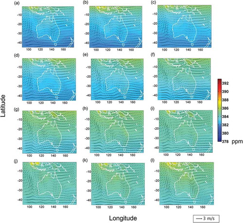
The vertical transport of CO₂ can be inferred from vertical motion given in Figure 6, where the two regions (i.e., southeastern Japan and southeastern Australia) have quite different characteristics. Both the maximum in April and the minimum in August are located near the ground level at southeastern Japan, suggesting the major sources and sinks of CO₂ should be located near the surface in this region (Figure 6(a)) (Gurney et al. 2002). The peak CO₂ concentration is found near the ground level between 900 and 700 hPa in April, just before the vegetation growing season, and this peak is delayed in time to May in the middle to upper levels between 600 and 400 hPa. The vertical distribution of carbon tracker CO₂ also explains the movement of the peak of CO₂ concentrations (Figure 6(c)). This suggests that CO₂ is transported vertically by large-scale atmospheric circulation, which is also explained by omega and horizontal winds. While the omega wind is positive (i.e., the descending motion) during November to April (Figure 6(e)), CO₂ concentration shows a strong gradient in vertical, thereby implying a suppressed vertical upward transport of CO₂ in this season. When the vertical motion changes into the ascending motion during May–September, the vertical stratification becomes weaker due to the increased vertical transport. We further examine the horizontal transport of CO₂ in this region in Figure 7. High CO₂ concentrations around northeastern China, where much of natural and anthropogenic CO₂ is emitted into the atmosphere, tend to move to the east by northwesterlies or westerlies from November to April (Figure 8(a–d,k,l). This flow pattern corresponds to the East Asian winter monsoon. During the active vegetation season from May to September, the oceanic region in East Asia is dominated by large-scale anticyclonic circulation. This pattern drives southerly or southwesterly flow over China and Korea, thereby transporting CO₂ to the north. This flow pattern corresponds to the East Asian summer monsoon. Note that CO₂ concentration decreases to the north during the active vegetation season from May to September, which is totally opposite to the case from November to April, with the maximum in the south and the minimum in the north. This suggests that the seasonal variation of CO₂ concentration is much higher in the boreal continent, presumably caused by much larger seasonal variation in vegetation (Shim, Lee, and Wang 2013; Fan et al. 1998; Angert et al. 2005; Van Breemen et al. 1998).

Figure 8. Monthly CO₂ concentration from carbon tracker and horizontal wind at 1000–700 hPa from NCEP reanalysis 2 data averaged during 2006–2011 at East Asia; (a) through (l) correspond to January–December.

Unlike the case of southeastern Japan, southeastern Australia in the Southern Hemisphere shows the maximum in October and the minimum in February. In addition, the highest concentration exists not near the ground level but above at 700 hPa (Figure 6(b)). This suggests that the column concentration is affected more by horizontal transport above the planetary boundary layer, rather than being affected by any significant sources or sinks at the ground. The vertical distribution and transport of CO₂ concentrations at southeastern Japan are not significantly related to the omega wind. Instead, the zonal wind transports relatively high CO₂ concentrations from the Northern Hemisphere to southeastern Australia area in the Southern Hemisphere. The movement and pattern of zonal wind correspond to the horizontal transport of CO₂ around Australia including the Indonesian and Papua New Guinean area (Figure 9). Unlike southeastern Japan (Figures 6(a,c)), the vertical motion of omega wind at southeastern Australia is downward all year around, which tends to suppress the vertical transport (Figure 6(e)). In the Southern Hemisphere, the meridional gradient of CO₂ concentration is consistent with the maxima in the equatorward and the minima in the poleward, although its gradient is largest in austral summer from January to April (Figure 9).

Figure 9. Monthly CO₂ concentration from carbon tracker and horizontal wind from NCEP reanalysis 2 data averaged during 2006–2011 in Australia including Indonesia and Papua New Guinea; (a) through (l) correspond to January–December.

Several studies have investigated the vertical transport of CO₂ (Crevoisier et al. 2009; Li et al. 2014; Lee, Im, and Lee 2015). Crevoisier et al. (2009) investigated the vertical transport of CO₂ from 0 to 20N using IASI and aircraft measurements. Nevertheless, this study did not explain factors that cause the vertical transport of CO₂. Kumar, Revadekar, and Tiwari (2014) proposed that vertical motion derived by convection may cause the vertical transport of CO₂ from surface to mid-troposphere using AIRS over India. However, since the vertical transport of CO₂ is mainly driven by vertical wind and dispersion, which vary by region, it should be investigated for various regions with different characteristics such as atmospheric conditions, geographical features, and climate conditions. Vegetation activities and phenology are crucial to control the quantity of CO₂ in the atmosphere, especially near the ground.

3.4. Comparison of monthly vertical variations between TES and CONTRAIL CO₂

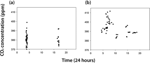
Figure 10 shows the vertical variation of monthly CO₂ between 2006 and 2011 at southeastern Japan using TES and CONTRAIL CO₂ concentration data. There was no data for some months: the number of TES CO₂ observations started to decrease since 2009 and JAL airplanes did not pass over southeastern Japan in certain months. While both TES- and CONTRAIL-derived CO₂ concentrations show a secular increasing trend with time, the seasonal cycle each year basically resembles the multiyear averaged one that is presented in Figure 10(a). It is intriguing that, although CO₂ concentrations at lower altitude (i.e., near 910 hPa; 850–950 m) in August are generally lowest because of active photosynthesis of vegetation (Figure 10(a)), the CONTRAIL data show exceptionally high values in August 2007, 2010, and 2011 (Figure 10(b)). It was found that there were many CONTRAIL samples collected during early morning for the months mentioned earlier, which showed relatively high CO₂ concentrations (>390 ppm) (Figure 11). Relatively high CO₂ concentration values in the early morning or nighttime (Li et al. 2014) by active respiration of terrestrial biosphere might cause the bias of overestimation in the time average. In addition, the nocturnal boundary layer is stable and suppresses the vertical dilution of CO₂. However, TES usually measured CO₂ concentration in August 2007 and 2010 in the morning, and thus, high CO₂ concentrations were not captured near the surface (Figure 11). Very limited sensitivity of TES CO₂ product near the ground level may also explain such discrepancy. The diurnal cycle might be more significant than other factors such as anthropogenic emissions and winds in the regional scale during summertime when CO₂ concentrations are relatively low on the ground.

Figure 10. CO₂ monthly vertical variation around southeastern Japan from 2006 to 2011. (a) TES CO₂ yearly variation. (b) CONTRAIL CO₂ yearly variation.

Figure 11. CO₂ concentrations measured by TES and CONTRAIL by time. (a) CO₂ concentrations measured by TES in August 2007 and 2010 around southeastern Japan. (b) CO₂ concentrations measured by CONTRAIL in August 2007 and 2010 around southeastern Japan.

4. Conclusions

This study compared various types of TIR-based satellite products and carbon tracker mole fraction data for CO₂ concentrations with the airborne CONTRAIL data. In addition, the vertical and horizontal distribution of CO₂ was examined in an attempt to understand the dynamical and physical mechanisms that drive such distribution. The comparison results varied by satellite product and the TES-derived CO₂ concentrations showed the best agreement with CONTRAIL data resulting in R² ~ 0.95, RMSE ~ 0.7 ppm, and bias ~–0.05 ppm. The AIRS-derived CO₂ concentrations also showed good agreement with CONTRAIL data while the TANSO-derived ones did not yield good agreement. The vertical distribution of CO₂ was investigated using TES and the large-scale winds from the atmospheric reanalysis, which revealed that the vertical distribution of CO₂ is significantly related to geophysical characteristics, vegetation phenology, land composition, and the emission of anthropogenic CO₂ from the surrounding areas. While the vertical distribution of CO₂ around southeastern Japan is largely controlled by horizontal and vertical winds, horizontal wind is a dominant factor ruling CO₂ transport around southeastern Australia. Finally, the results showed that TIR-derived CO₂ concentrations at lower altitudes might not be able to represent the diurnal cycle of CO₂ and thus special care should be given when using such satellite-derived products. In order to better understand the dynamics of atmospheric CO₂ at the mesoscale level, the emission of CO₂, meteorological environment, and geophysical characteristics of a region should be carefully considered.

Acknowledgments

This research was supported by Technology Development Program to Solve Climate Changes through the National Foundation of Korea (NRF) funded by the Ministry of Science, ICT, & Future Planning of Korea (Grant: NRF-2012M1A2A2671851), and “Development of satellite based ocean carbon flux model for seas around Korea” funded by the Ministry of Ocean and Fisheries, Republic of Korea. The authors are thankful to the CONTRAIL team (PIs: Toshinobu Machida, Hidekazu Matsueda, and Tousuke Sawa) in Japan for providing airborne CO₂ observation data.

Disclosure statement

No potential conflict of interest was reported by the authors.

Additional information

Funding

This research was supported by Technology Development Program to Solve Climate Changes through the National Foundation of Korea (NRF) funded by the Ministry of Science, ICT, & Future Planning of Korea [Grant: NRF-2012M1A2A2671851], and “Development of satellite based ocean carbon flux model for seas around Korea” funded by the Ministry of Ocean and Fisheries, Republic of Korea.

References

- Angert, A., S. Biraud, C. Bonfils, C. C. Henning, W. Buermann, J. Pinzon, and I. Fung. 2005. “Drier Summers Cancel Out the CO2 Uptake Enhancement Induced by Warmer Springs.” Proceedings of the National Academy of Sciences of the United States of America 102: 10823–10827. doi:10.1073/pnas.0501647102.
- Aumann, H. H., and T. S. Pagano. 2003. Early Results from AIRS on the EOS, International Symposium on Remote Sensing, Crete, Greece, 131–136.
- Baldocchi, D., E. Falge, L. Gu, and R. Olson. 2001. “FLUXNET: A New Tool to Study the Temporal and Spatial Variability of Ecosystem-Scale Carbon Dioxide, Water Vapor, and Energy Flux Densities.” Bulletin of the American Meteorological Society 82: 2415. doi:10.1175/1520-0477(2001)082<2415:FANTTS>2.3.CO;2.
- Bréon, F.-M., and P. Ciais. 2010. “Spaceborne Remote Sensing of Greenhouse Gas Concentrations.” Comptes Rendus Geoscience 342: 412–424. doi:10.1016/j.crte.2009.09.012.
- Ceos, C. 2014. “Strategy for Carbon Observations from Space.” The Committee on Earth Observation Satellites (CEOS) Response to the Group on Earth Observations (GEO) Carbon Strategy. (Issued Date: September 30: 2014.
- Chahine, M. T., L. Chen, P. Dimotakis, X. Jiang, Q. Li, E. T. Olsen, T. Pagano, J. Randerson, and Y. L. Yung. 2008. “Satellite Remote Sounding of Mid-Tropospheric CO2.” Geophysical Research Letters 35: L17807. doi:10.1029/2008GL035022.
- Chédin, A., R. Saunders, A. Hollingsworth, N. Scott, M. Matricardi, J. Etcheto, C. Clerbaux, R. Armante, and C. Crevoisier. 2003. “The Feasibility of Monitoring CO2 from High-Resolution Infrared Sounders.” Journal of Geophysical Research: Atmospheres 108: 4064. doi:10.1029/2001JD001443.
- Chevallier, F., F.-M. Bréon, and P. J. Rayner. 2007. “Contribution of the Orbiting Carbon Observatory to the Estimation of CO2 Sources and Sinks: Theoretical Study in a Variational Data Assimilation Framework.” Journal of Geophysical Research: Atmospheres 112: D09307. doi:10.1029/2006JD007375.
- Crevoisier, C., A. Chédin, H. Matsueda, T. Machida, R. Armante, and N. A. Scott. 2009. “First Year of Upper Tropospheric Integrated Content of CO2 from Iasi Hyperspectral Infrared Observations.” Atmos Chemical Physical 9: 4797–4810. doi:10.5194/acp-9-4797-2009.
- Crisp, D., R. M. Atlas, F. M. Breon, L. R. Brown, J. P. Burrows, P. Ciais, and C. E. Miller. 2004. “The Orbiting Carbon Observatory (OCO) Mission.” Advances in Space Research 34: 700–709. doi:10.1016/j.asr.2003.08.062.
- Crisp, D., B. M. Fisher, C. O’Dell, C. Frankenberg, R. Basilio, H. Bösch, L. R. Brown, et al. 2012. “The Acos CO2 Retrieval Algorithm - Part Ii: Global XCO2 Data Characterization”. Atmos Measurement Technical 5: 687–707. doi:10.5194/amt-5-687-2012.
- Ding, M. 2016. “Temperature Dependence Of Variations In The End Of The Growing Season From 1982 To 2012 On The Qinghai–tibetan Plateau.” Giscience & Remote Sensing 53 (2): 147–163. doi: 10.1080/15481603.2015.1120371.
- Emmons, L. K., M. N. Deeter, J. C. Gille, D. P. Edwards, J. L. Attié, J. Warner, and J. F. Lamarque. 2004. “Validation of Measurements of Pollution in the Troposphere (MOPITT) CO Retrievals with Aircraft in Situ Profiles.” Journal of Geophysical Research: Atmospheres 109: D3. doi:10.1029/2003JD004101.
- Engelen, R. J., and G. L. Stephens. 2004. “Information Content of Infrared Satellite Sounding Measurements with respect to CO2.” Journal of Applied Meteorology 43: 373–378. doi:10.1175/1520-0450(2004)043<0373:ICOISS>2.0.CO;2.
- Fan, S., M. Gloor, J. Mahlman, S. Pacala, J. Sarmiento, T. Takahashi, and P. Tans. 1998. “A Large Terrestrial Carbon Sink in North America Implied by Atmospheric and Oceanic Carbon Dioxide Data and Models.” Science 282: 442–446. doi:10.1126/science.282.5388.442.
- Forkel, M., N. Carvalhais, C. Rödenbeck, R. Keeling, M. Heimann, K. Thonicke, S. Zaehle, and M. Reichstein. 2016. “Enhanced Seasonal CO2 Exchange Caused by Amplified Plant Productivity in Northern Ecosystems.” Science 351: 696–699. doi:10.1126/science.aac4971.
- Forster, P., V. Ramaswamy, P. Artaxo, T. Berntsen, R. Betts, D. W. Fahey, J. Haywood, et al. 2007. Changes in Atmospheric Constituents and in Radiative Forcing, 129–234. Cambridge, United Kingdom: Cambridge University Press.
- Foucher, P. Y., A. Chédin, R. Armante, C. Boone, C. Crevoisier, and P. Bernath. 2011. “Carbon Dioxide Atmospheric Vertical Profiles Retrieved from Space Observation Using ACE-FTS Solar Occultation Instrument.” Atmospheric Chemistry and Physics 11: 2455–2470. doi:10.5194/acp-11-2455-2011.
- Garbulsky, M. F., J. Peñuelas, D. Papale, and I. Filella. 2008. “Remote Estimation of Carbon Dioxide Uptake by a Mediterranean Forest.” Global Change Biology 14: 2860–2867. doi:10.1111/gcb.2008.14.issue-12.
- Gurney, K. R., D. Baker, P. Rayner, and S. Denning. 2008. “Interannual Variations in Continental-Scale Net Carbon Exchange and Sensitivity to Observing Networks Estimated from Atmospheric CO2 Inversions for the Period 1980 to 2005.” Global Biogeochemical Cycles 22: GB3025. doi:10.1029/2007GB003082.
- Gurney, K. R., R. M. Law, A. S. Denning, P. J. Rayner, D. Baker, P. Bousquet, and I. Y. Fung. 2002. “Towards Robust Regional Estimates of CO2 Sources and Sinks Using Atmospheric Transport Models.” Nature 415: 626–630. doi:10.1038/415626a.
- Harazono, Y., M. Mano, A. Miyata, R. C. Zulueta, and W. C. Oechel. 2003. “Inter‐Annual Carbon Dioxide Uptake of a Wet Sedge Tundra Ecosystem in the Arctic.” Tellus B 55: 215–231. doi:10.1034/j.1600-0889.2003.00012.x.
- Imasu, R., N. Saitoh, Y. Niwa, H. Suto, A. Kuze, K. Shiomi, and M. Nakajima. 2008. In Radiometric Calibration Accuracy of GOSAT-TANSO-FTS (TIR) Relating to Co2 Retrieval Error, In Asia-Pacific Remote Sensing. International Society for Optics and Photonics. 71490B-71490B.
- Inoue, M., I. Morino, O. Uchino, Y. Miyamoto, Y. Yoshida, T. Yokota, T. Machida, et al. 2013. “Validation of Xco2 Derived from SWIR Spectra of GOSAT TANSO-FTS with Aircraft Measurement Data”. Atmospheric Chemistry and Physics 13: 9771–9788. doi:10.5194/acp-13-9771-2013.
- Jiang, X., J. Wang, E. T. Olsen, M. Liang, T. S. Pagano, L. L. Chen, S. J. Licata, and Y. L. Yung. 2012. “Influence of El Niño on Midtropospheric CO2 from Atmospheric Infrared Sounder and Model.” Journal of the Atmospheric Sciences 70: 223–230. doi:10.1175/JAS-D-11-0282.1.
- Kanamitsu, M., W. Ebisuzaki, J. Woollen, S.-K. Yang, J. J. Hnilo, M. Fiorino, and G. L. Potter. 2002. “Ncep–Doe Amip-Ii Reanalysis (R-2).” Bulletin of the American Meteorological Society 83: 1631–1643. doi:10.1175/BAMS-83-11-1631.
- Keeling, C. D., J. F. S. Chin, and T. P. Whorf. 1996. “Increased Activity of Northern Vegetation Inferred from Atmospheric CO2 Measurements.” Nature 382: 146–149. doi:10.1038/382146a0.
- Keeling, C. D., S. C. Piper, and M. Heimann. 2013. “A Three-Dimensional Model of Atmospheric CO2 Transport Based on Observed Winds: 4. Mean Annual Gradients and Interannual Variations.” In Aspects of Climate Variability in the Pacific and the Western Americas, Edited by Peterson, D.H. 305–363. Washington DC: American Geophysical Union.
- Kim, H. O. 2015. “Sensitivity Of Vegetation Indices To Spatial Degradation Of Rapideye Imagery For Paddy Rice Detection: A Case Study Of South Korea.” Giscience & Remote Sensing 52 (1): 1–17. doi: 10.1080/15481603.2014.1001666.
- Kulawik, S. S., D. B. A. Jones, R. Nassar, F. W. Irion, J. R. Worden, K. W. Bowman, and M. L. Fischer. 2010. “Characterization of Tropospheric Emission Spectrometer (TES) CO2 for Carbon Cycle Science.” Atmospheric Chemistry and Physics 10: 5601–5623. doi:10.5194/acp-10-5601-2010.
- Kulawik, S. S., J. R. Worden, S. C. Wofsy, S. C. Biraud, R. Nassar, D. B. A. Jones, E. T. Olsen, et al. 2013. “Comparison of Improved Aura Tropospheric Emission Spectrometer CO2 with Hippo and SGP Aircraft Profile Measurements”. Atmospheric Chemistry and Physics 13: 3205–3225. doi:10.5194/acp-13-3205-2013.
- Kumar, K. R., J. V. Revadekar, and Y. K. Tiwari. 2014. “Airs Retrieved CO2 and Its Association with Climatic Parameters over India during 2004–2011.” Science of the Total Environment, 476–477 (79–89): 79–89. doi:10.1016/j.scitotenv.2013.12.118.
- Kuze, A., H. Suto, M. Nakajima, and T. Hamazaki. 2009. “Thermal and near Infrared Sensor for Carbon Observation Fourier-Transform Spectrometer on the Greenhouse Gases Observing Satellite for Greenhouse Gases Monitoring.” Applied Optics 48: 6716–6733. doi:10.1364/AO.48.006716.
- Lee, S., J. Im, and M. I. Lee. 2015. The Spatiotemporal Variations of CO2 in the Troposphere Using Multi-Sensor Satellite Data and Aircraft Observations, Geoscience and Remote Sensing Symposium (IGARSS), 2015 IEEE International: Milan. 26-31 July 2015. 2214–2217.
- Li, Y., J. Deng, C. Mu, Z. Xing, and K. Du. 2014. “Vertical Distribution of CO2 in the Atmospheric Boundary Layer: Characteristics and Impact of Meteorological Variables.” Atmospheric Environment 91: 110–117. doi:10.1016/j.atmosenv.2014.03.067.
- Machida, T., H. Matsueda, Y. Sawa, Y. Nakagawa, K. Hirotani, N. Kondo, K. Goto, T. Nakazawa, K. Ishikawa, and T. Ogawa. 2008. “Worldwide Measurements of Atmospheric CO2 and Other Trace Gas Species Using Commercial Airlines.” Journal of Atmospheric and Oceanic Technology 25 (1744–1754.1): 1744–1754. doi:10.1175/2008JTECHA1082.1.
- Maddy, E. S., C. D. Barnet, M. Goldberg, C. Sweeney, and X. Liu. 2008. “CO2 Retrievals from the Atmospheric Infrared Sounder: Methodology and Validation.” Journal of Geophysical Research: Atmospheres 113: D11301. doi:10.1029/2007JD009402.
- Miller, C. E., D. Crisp, P. L. DeCola, S. C. Olsen, J. T. Randerson, A. M. Michalak, and D. B. A. Jones. 2007. “Precision Requirements for Space‐Based Data.” Journal of Geophysical Research: Atmospheres 112: D10. doi:10.1029/2006JD007659.
- Mutanga, O., and A. K. Skidmore. 2004. “Narrow Band Vegetation Indices Overcome the Saturation Problem in Biomass Estimation.” International Journal of Remote Sensing 25: 3999–4014. doi:10.1080/01431160310001654923.
- Myneni, R. B., J. Dong, C. J. Tucker, R. K. Kaufmann, P. E. Kauppi, J. Liski, L. Zhou, V. Alexeyev, and M. K. Hughes. 2001. “A Large Carbon Sink in the Woody Biomass of Northern Forests.” Proceedings of the National Academy of Sciences 98: 14784–14789. doi:10.1073/pnas.261555198.
- Nassar, R., D. B. A. Jones, S. S. Kulawik, J. R. Worden, K. W. Bowman, R. J. Andres, P. Suntharalingam, et al. 2011. “Inverse Modeling of CO2 Sources and Sinks Using Satellite Observations of CO2 from TES and Surface Flask Measurements”. Atmospheric Chemistry and Physics 11: 6029–6047. doi:10.5194/acp-11-6029-2011.
- Nassar, R., J. A. Logan, H. M. Worden, I. A. Megretskaia, K. W. Bowman, G. B. Osterman, and M. K. Dubey. 2008. “Validation of Tropospheric Emission Spectrometer (TES) Nadir Ozone Profiles Using Ozonesonde Measurements.” Journal of Geophysical Research: Atmospheres 113: D15. doi:10.1029/2007JD008819.
- Numata, K., J. R. Chen, S. T. Wu, J. B. Abshire, and M. A. Krainak. 2011. “Frequency Stabilization of Distributed-Feedback Laser Diodes at 1572 Nm for Lidar Measurements of Atmospheric Carbon Dioxide.” Applied Optics 50: 1047–1056. doi:10.1364/AO.50.001047.
- O’Dell, C. W., B. Connor, H. Bösch, D. O’Brien, C. Frankenberg, R. Castano, and M. Gunson. 2012. “Corrigendum To” the ACOS CO 2 Retrieval Algorithm–Part 1: Description and Validation against Synthetic Observations. Atmospheric Measurement Techniques 5, 99–121, 2012.” Atmospheric Measurement Techniques 5: 193–193. doi:10.5194/amt-5-193-2012.
- Olsen, T. S. 2009. “AIRS Version 5 Release Tropospheric CO2 Products.” Jet Propulsion Laboratory. Available online: https://disc.gsfc.nasa.gov/AIRS/documentation/AIRS-V5-Tropospheric-CO2-Products.pdf (accessed on 15 December 2009)
- Pagano, T. S., M. T. Chahine, and E. T. Olsen. 2011. “Seven Years of Observations of Mid-Tropospheric CO2 from the Atmospheric Infrared Sounder.” Acta Astronautica 69: 355–359. doi:10.1016/j.actaastro.2011.05.016.
- Patra, P., R. M. Law, W. Peters, C. Rödenbeck, M. Takigawa, C. Aulagnier, and L. Bruhwiler. 2008. “Transcom Model Simulations of Hourly Atmospheric CO2: Analysis of Synoptic‐Scale Variations for the Period 2002–2003.” Global Biogeochemical Cycles 22. doi:10.1029/2007GB003081.
- Peters, W., A. R. Jacobson, C. Sweeney, A. E. Andrews, T. J. Conway, K. Masarie, J. B. Miller, et al. 2007. “An Atmospheric Perspective on North American Carbon Dioxide Exchange: Carbontracker”. Proceedings of the National Academy of Sciences 104: 18925–18930. doi:10.1073/pnas.0708986104.
- Rodgers, C. 2000. Inverse Methods for Atmospheric Sounding: Theory and Practice (Vol. 2)., Singapore:World Scientific.1-238.
- Sawa, Y., T. Machida, and H. Matsueda. 2012. “Aircraft Observation of the Seasonal Variation in the Transport of CO2 in the Upper Atmosphere.” Journal of Geophysical Research: Atmospheres 117: D05305. doi:10.1029/2011JD016933.
- Shim, C., J. Lee, and Y. Wang. 2013. “Effect of Continental Sources and Sinks on the Seasonal and Latitudinal Gradient of Atmospheric Carbon Dioxide over East Asia.” Atmospheric Environment 79: 853–860. doi:10.1016/j.atmosenv.2013.07.055.
- Sioris, C. E., C. D. Boone, R. Nassar, K. J. Sutton, I. E. Gordon, K. A. Walker, and P. F. Bernath. 2014. “Retrieval of Carbon Dioxide Vertical Profiles from Solar Occultation Observations and Associated Error Budgets for ACE-FTS and CASS-FTS.” Atmospheric Measurement Techniques 7: 2243–2262. doi:10.5194/amt-7-2243-2014.
- Stephens, B. B., K. R. Gurney, P. P. Tans, C. Sweeney, W. Peters, L. Bruhwiler, and S. Aoki. 2007. “Weak Northern and Strong Tropical Land Carbon Uptake from Vertical Profiles of Atmospheric CO2.” Science 316: 1732–1735. doi:10.1126/science.1137004.
- Sweeney, C., A. Karion, S. Wolter, T. Newberger, D. Guenther, J. A. Higgs, A. E. Andrews et al. 2015. “Seasonal Climatology of CO2 across North America from Aircraft Measurements in the NOAA/ESRL Global Greenhouse Gas Reference Network.” Journal of Geophysical Research: Atmospheres 120:2014JD022591.
- Tian, H., J. M. Melillo, D. W. Kicklighter, S. Pan, J. Liu, A. D. McGuire, and B. Moore. 2003. “Regional Carbon Dynamics in Monsoon Asia and Its Implications for the Global Carbon Cycle.” Global and Planetary Change 37: 201–217.
- Van Breemen, N., A. Jenkins, R. F. Wright, D. J. Beerling, W. J. Arp, F. Berendse, and P. S. Verburg. 1998. “Impacts of Elevated Carbon Dioxide and Temperature on a Boreal Forest Ecosystem (CLIMEX Project).” Ecosystems 1: 345–351. doi:10.1007/s100219900028.
- Yagci, A. 2015. “The Effect Of Corn-soybean Rotation On The Ndvi-based Drought Indicators: A Case Study In Iowa, Usa, Using Vegetation Condition Index”. Giscience & Remote Sensing, 52 (3): 290–314. doi:10.1080/15481603.2015.1038427.
- Yokota, T., Y. Yoshida, N. Eguchi, Y. Ota, T. Tanaka, H. Watanabe, and S. Maksyutov. 2009. “Global Concentrations of CO2 and Ch4 Retrieved from GOSAT: First Preliminary Results.” Sola 5: 160–163. doi:10.2151/sola.2009-041.
- Yoshida, Y., N. Kikuchi, I. Morino, O. Uchino, S. Oshchepkov, A. Bril, T. Saeki, et al. 2013. “Improvement of the Retrieval Algorithm for GOSAT SWIR XCO2 and XCH4 and Their Validation Using TCCON Data”. Atmospheric Measurement Techniques 6: 1533–1547. doi:10.5194/amt-6-1533-2013.
- Yoshida, Y., N. Kikuchi, and T. Yokota. 2012. “On-Orbit Radiometric Calibration of SWIR Bands of TANSO-FTS Onboard GOSAT.” Atmospheric Measurement Techniques 5: 2515–2523. doi:10.5194/amt-5-2515-2012.
- Zhang H, Q. Li, J. Liu, J. Shang, X. Du, L. Zhao, N. Wang, and T. Dong. 2017. “Crop Classification And Acreage Estimation In North Korea Using Phenology Features.”. Giscience & Remote Sensing 54 (3): 1–26. doi:10.1080/15481603.2016.1276255.