Utilization of Landsat data to quantify land-use and land-cover changes related to oil and gas activities in West-Central Alberta from 2005 to 2013

Abstract

Land use and land cover (LULC) change detection associated with oil and gas activities plays an important role in effective sustainable management practices, compliance monitoring, and reclamation assessment. In this study, a mapping methodology is presented for quantifying pre- and post-disturbance LULC types with annual Landsat Best-Available-Pixel multispectral data from 2005 to 2013. Annual LULC and land disturbance maps were produced for one of the major conventional oil and gas production areas in West-Central Alberta with an accuracy of 78% and 87%, respectively. The highest rate of vegetation loss (178 km²/year) was observed in coniferous forest compared to broadleaf forest, mixed forest, and native vegetation. Integration of ancillary oil and gas geospatial data with annual land disturbances indicated that less than 20% of the total land disturbances were attributable to oil and gas activities. In 2013, approximately 44% of oil and gas disturbances from 2005 to 2013 showed evidence of vegetation recovery. In the future, geospatial data related to wildfire, logging activities, insect defoliation, and other natural and anthropogenic factors can be integrated to quantify other causes of land disturbances.

Keywords:

• change detection
• classification
• land disturbance
• vegetation loss
• vegetation recovery
• West-Central Alberta

Introduction

Large area planning associated with natural resource development requires spatially explicit data on land use and land cover (LULC) composition and the extent that contributes to contemporary change (Powers et al. 2015, Zhang et al. 2014). Detection and attribution of disturbance agent, such as the presence of anthropogenic change associated with oil and gas activities, plays an important role in the development of effective sustainable management practices, compliance monitoring, and reclamation performance assessment. Earth Observation (EO) data allow us to detect possible long-term changes in LULC related to industrial infrastructure (e.g., roads, well pads, pipeline corridors, processing facilities, core hole drilling sites, and access corridors to core hole sites) and transient land disturbances (e.g., cutblock) associated with oil and gas exploration and extraction. Quantification of these landscape changes using EO data is a transparent, repeatable, and spatially explicit means to supplement and guide compliance assurance activities, which include site visits by agency personnel that is both time consuming and costly.

The magnitude and diffuse nature of landscape disturbance and fragmentation determines the restoration process of the vegetation ecosystem. For instance, wildfire-impacted boreal forest usually recovers within 10 years, but a landscape altered by oil and gas activity (e.g., establishment of well sites, access roads, and seismic lines) can take decades to recover (Powers et al. 2015; Osko and MacFarlane 2001; Schneider 2002). Large area land-cover variations and long-term patterns associated with anthropogenic disturbances were previously studied using Landsat (TM and ETM+) satellite imagery (Powers et al. 2015; Gillanders et al. 2008; Potapov, Turubanova, and Hansen 2011; Schroeder et al. 2011; Hobson and Bayne 2000; Meddens et al. 2008; Linke et al. 2005). Quantification of land-cover changes using multi-temporal Landsat datasets can be applied to study deforestation, damage assessment, disaster monitoring, urban expansion, planning, and land management (Hussain et al. 2013; Grekousis, Mountrakis, and Kavouras 2015). Knowledge of change agent is important to ensure correct attribution and definition of a given disturbance, as well as to guide assessment and remediation activities. Over forest landscapes, a number of natural and anthropogenic disturbance agents operate. Natural disturbances can occur as a result of insects or wildfire. These agents typically result in a land temporary change in land cover, but not to land use. Industrial activity, such as related to oil and gas exploration and extraction activity, has a land-cover change and often an associated change in land use. For instance, for deforestation to have occurred, a change in both land cover and land use is required (e.g., forest harvesting [logging] is not deforestation). Areas disturbed by harvesting are subject to provincial regulations covering harvesting practices and subsequent monitoring of regeneration and/or replanting activities. Similarly, oil and gas exploration and extraction activities are monitored by appropriate agencies to ensure implementation of and compliance to relevant practices and requirements.

Several approaches have been undertaken to map anthropogenic disturbances from satellite imagery that include an emphasis on well sites (He et al. 2009; Baker et al. 2013; Pasher, Seed, and Duffe 2013; Salehi et al. 2014; Pouliot and Latifovic 2016). Anthropogenic disturbance mapping by manually digitizing airborne or spaceborne imagery is time consuming and laborious and is not a realistic approach for long-term monitoring, although manual digitization does not usually require any image processing, e.g., atmospheric correction and image-to-image color balancing (Salehi et al. 2014; Pasher, Seed, and Duffe 2013). Anthropogenic footprint extraction using very high-resolution satellite imagery is often done by resampling it to a more coarse resolution, e.g., resampling 1-m spatial resolution to 5–30-m spatial resolution data (Baker et al. 2013). Salehi et al. (2014) introduced a combination of object-based and pixel-based approaches to extract well sites from Landsat-5 imagery and concluded that, while a pixel-based approach is not statistically different from an object-based approach when using coarser spatial resolution data (30 m), an object-based approach outperforms the pixel-based approach where high-resolution data (1 m) are used. For long-term (e.g., annual) anthropogenic change detection over a large area, utilization of freely available medium spatial resolution (30 m) Landsat datasets are a more practical approach than the utilization of very high spatial resolution (1 m) datasets considering both the temporal and spatial extent of disturbances under investigation (Salehi et al. 2014; He et al. 2009). The objective of this study is to characterize annual land disturbance associated with both anthropogenic activities and natural causes with the aid of annual LULC classification maps (2005–2013) using Landsat multispectral data.

Information extraction from multispectral or hyperspectral imagery requires pre-processing, e.g., calibration, assessment and removal of sensor artifacts, and removal of atmospheric effects. Some of the common information extraction methods include supervised classification, spectral unmixing, spectral matching, feature fitting, and matched filtering (Jensen 2004). In the literature, common supervised classification methods include Maximum Likelihood (ML; Richards 1999), Artificial Neural Network (ANN; Atkinson and Tatnall 1997), Support Vector Machine (SVM; Pal and Mather 2005), and Decision Tree (Hansen, Dubayah, and Defries 1996). In this study, ML is selected for LULC classification since it is widely used and has generally faster processing times compared to advanced classifiers, e.g., SVM and ANN, although SVM and ANN outperform ML in terms of classification accuracy (Pal and Mather 2005; Waske and Benediktsson 2007; Shafri, Suhaili, and Mansor 2007). Faster processing time plays an important role when considering large study areas (of millions of hectares), further exaggerated when incorporating multi-temporal investigations. ML is a parametric classifier that considers variance and covariance within class distributions for normally distributed data (Inc 1999; Otukei and Blaschke 2010). In this study, classification of vegetation and transient LULC types are conducted with ML. Since supervised classifiers are often unable to extract small anthropogenic footprints, e.g., well pads, a target detection approach is employed to extract sub-pixel-level anthropogenic footprints. Commonly used target detection algorithms include Orthogonal Subspace Projection (OSP; Harsanyi and Chang 1994), Constraint Energy Minimization (CEM; Chang et al. 2000; Farrand et al. 1997), and Matched Filter (MF; Boardman, Kruse, and Green 1995). In this study, CEM is chosen for anthropogenic footprint extraction since it usually eliminates unidentified signal sources, suppresses noise better than OSP, and does not require a data mean to be subtracted from all pixel vectors unlike MF (Boardman, Kruse, and Green 1995; Chang et al. 2000; Du, Ren, and Chang 2003; Arora et al. 2013; Ji et al. 2015). Spectral Angle Mapper (SAM; Kruse et al. 1993) is a widely used spectral similarity measure due to its low sensitivity to pixel illumination. SAM assumes that the lines connecting the origin and each spectrum point are the vectors of the direction of the spectra corresponding to the range of possible illuminations with all possible positions of the materials (Kruse et al. 1993; Staenz et al. 1999). A pixel with poor illumination will fall closer to the origin than a pixel with greater illumination, although both pixels might have the same reflectance characteristics. Accordingly, SAM is insensitive to changes in pixel illumination as increasing or decreasing illumination only changes the magnitude, not the direction. In this study, CEM–SAM partial unmixing ratio is taken to minimize false detection of anthropogenic footprints. Annual LULC classification maps from 2005 to 2013 are produced by combining the results from ML and CEM–SAM. Normalized Difference Built-up Index (NDBI) was previously used in the literature to identify urban and build-up areas as well as to detect land changes (Zha, Gao, and Ni 2003; Chen et al. 2006; Pouliot and Latifovic 2016). The objective of this research was twofold; the first was to extract and classify year-to-year land disturbance and vegetation loss with the state of cumulative disturbances using annual Landsat data from 1985 to 2013. The second objective was to estimate types of land disturbance, vegetation loss, and evidence of vegetation recovery associated with oil and gas footprints based on ancillary geospatial data.

Study area and datasets

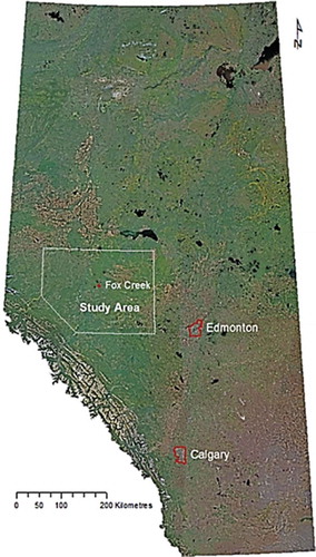
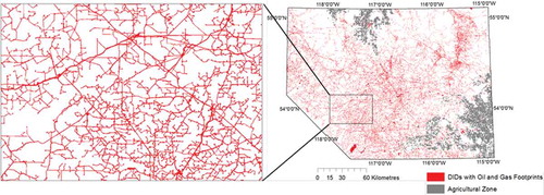
The study area is located approximately 200 km northwest of Edmonton, Alberta, Canada, as shown in Figure 1, represents one of the major conventional oil and gas production sites with an area of 43,164 km², and has additional potential for unconventional oil and gas development (ERCB (Energy Resources Conservation Board) 2012).

Figure 1. Location of the study area in West-Central Alberta. For full color versions of the figures in this paper, please see the online version.

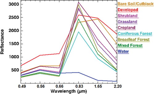
Pre-release versions of annual Landsat Best-Available-Pixel (BAP) multispectral data from 2005 to 2011 with 30-m spatial resolution were obtained from the Pacific Forestry Centre, Natural Resources Canada, for testing purposes and were used in this study (White et al. 2014). These datasets include Blue (0.49 µm), Green (0.56 µm), Red (0.66 µm), Near Infrared (NIR) (0.83 µm), Short-Wave Infrared (SWIR) 1 (1.65 µm), and SWIR 2 (2.2 µm) bands. In addition, publicly available Landsat BAP multispectral datasets for 2012 and 2013 with 30-m spatial resolution obtained from the Department of Geographical Sciences, University of Maryland, were utilized, which includes Red (0.66 µm), NIR (0.83 µm), SWIR 1 (1.65 µm), and SWIR 2 (2.2 µm) bands (Hansen et al. 2013).

Methods

This section outlines extraction of LULC changes from annual Landsat BAP data (2005–2013) that requires several processing steps including selection of ground-reference data, classification of LULC types, and extraction and attribution of land disturbances. Annual LULC map was generated with ML classifier and CEM–SAM partial unmixing method. Land-change detection maps were produced based on year-to-year changes in NDBI and were integrated with LULC maps and ancillary oil and gas footprints to assess pre- and post-disturbance condition as well as the sign of vegetation recovery from cumulative disturbances.

Ground-reference data selection

Two LULC datasets were utilized to select the ground-reference data for each year. The first dataset includes shrubland, grassland, agricultural, coniferous forest, and broadleaf forest land-cover types that were selected from a composition of two land-cover datasets of 2010 from the Canadian Forest Service and Agriculture and Agri-Food Canada that were compiled by the Alberta Biodiversity Monitoring Institute (Castilla et al. 2014; Alberta Biodiversity Monitoring Institute 2015). This dataset was used as one of the training datasets for the ML classifier. The second dataset includes oil and gas facilities/buildings of 2010 that were utilized to produce ground-reference data (Government of Alberta 2015). Average spectrum of the oil and gas facilities/buildings was used to train the CEM–SAM method to detect developed, mixed-developed, and transitional bare surface footprints. Since both datasets are available from 2010, this year was selected as the base year. Land-cover changes from target year to base year are detected with a simple difference in their NDBI values. Ground-reference data for each target year are generated by removing changed areas from the base ground-reference map as illustrated in Figure 2. Ground-reference data from the first and second dataset were selected with stratified random sampling with 10% minimum sample size from 43,164 km² area in order to minimize the processing time, where 30% of ground-reference data were selected for training and the remaining were selected for validation. Training data for ML classifier with cutblock/bare soil, mixed forest, and water were manually selected from the scene with visual analysis and were not used for validation. Areas with cloud, haze, cloud shadow, and noise were discarded from the ground-reference data. Cumulative land disturbances from 2005 to 2013 were validated using the forest disturbance data from Hansen et al. (2013) as a subset of all disturbances.

Figure 2. Processing steps to select ground-reference data for target year.

ML classifier

ML is a parametric classifier that assumes normality for the training samples and builds probability density functions for each class (Richards 1999; Hagner and Reese 2007; Sun et al. 2013). It classifies each pixel based on the relative probability of the pixel occurring within the probability density function of each class, which means each pixel is assigned to the class that has the highest probability value. According to Bayesian formula, the posterior probability $P\left(W_j/x\right)$of class j for W predefined classes with b bands of unclassified image is defined as

(1) $P\left(\frac{W_j}{x}\right)=\frac{P\left({\frac{x}{W}}_j\right)P\left(W_j\right)}{P\left(x\right)}$(1)

where $x={\left[x_1,x_2,\dots ,x_b\right]}^T$ in Equation (1) is the vector of a pixel, $P\left(W_j\right)$ is the prior probability of class j, and $P\left(x/W_j\right)$ is the conditional probability of observing x from $W_j$(probability density function). The discriminant function is expressed as

(2) $M_j\left(x\right)=lnP(W_j)+ln\frac{{\left|C_j^{-1}\right|}^{\frac{1}{2}}}{{\left(2\pi \right)}^{\frac{b}{2}}}-\frac{1}{2}{\left(x-{\mu }_j\right)}^T{C}_j^{-1}\left(x-{\mu }_j\right)$(2)

where $M_j\left(x\right)$ in Equation (2) is the likelihood function of x belonging to class j, ${\mu }_j$ is the mean vector of class j and $C_j$ is the covariance matrix of class j that plays a key role in discriminant analysis and accounts for the shape, size, and orientation of classes in the feature space.

CEM and SAM

CEM only requires prior knowledge of target spectra and employs a Finite Impulse Response (FIR) filter to constrain the desired target signature by a specific gain while minimizing the total energy of the output of other unknown signatures (Chang et al. 2000; Ji et al. 2015). CEM assumes the desired signature s as a priori with a finite set of observations $K=\left\{k_1,k_2,\dots ,k_N\right\}$, where $k_i=(k_{i1},k_{i2},\dots ,k_{iB}{)}^T$ is a pixel vector for 1 ≤ i ≤ N, N is the total number of pixels, and B is the total number of bands. It considers an FIR linear filter, $r=(r_1,r_2,\dots ,r_B{)}^T$, as a B-dimensional vector and minimizes the output energy subject to the unity constraint, $s^{T}r={\displaystyle \sum _{i=1}^B{s}_i{r}_i=1}$. The problem is described as

(3) $\underset{r}{\text{min}}\left(\frac{1}{N}\left[{\displaystyle \sum _{n=1}^N{\left(r^T{k}_i\right)}^2}\right]\right)=\underset{r}{\text{min}}\left(r^{T}Lr\right),$(3)

(4) $r_{CEM}=\frac{L^{-1}s}{s^T{L}^{-1}s}.$(4)

Equation (3) is subject to $s^{T}r=1$, where $L=\left(\frac{1}{N}\right){\displaystyle {\sum }_{n=1}^N{k}_i{k}_i{ }^T}$ is an autocorrelation matrix of K. Solution of Equation (3) is the CEM operator with a weight vector as described in Equation (4).

SAM calculates the angle between a reference spectrum and the spectrum to be matched in a B-dimensional space, where a smaller angle indicates a closer match (Kruse et al. 1993; Staenz et al. 1999). The angle is calculated as follows:

(5) $SAM=\mathrm{c}\mathrm{o}{\mathrm{s}}^{-1}\left(\frac{{\sum }_{b=1}^B{t}_b{x}_b}{\sqrt{{\sum }_{b=1}^B{t}_b^2{\sum }_{b=1}^B{x}_b^2}}\right)$(5)

where and in Equation (5) are the amplitudes of the reference spectrum and the spectrum to be matched in band b, respec tively.

Annual LULC classification

For each year, Equations (4) and (5) are applied to the Minimum Noise Fraction (Green et al. 1988) components derived from the Landsat BAP multispectral data with a mean spectrum of training anthropogenic footprints as discussed in the ground-reference data selection. Following steps are applied to convert the CEM/SAM ratio to a classification map with hierarchical layers of anthropogenic footprints and are exemplified in Figures 3 and 4.

Figure 3. Extraction and refinement process of anthropogenic footprints.

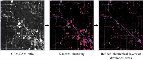
Figure 4. Work flow of fused classification map production.

1. Produce a CEM–SAM partial unmixing ratio map to suppress false positives and to enhance true positives based on the MF/SAM ratio approach described by Baiocchi et al. (2012) and EXELIS Visual Information Solutions (2015).

2. Convert the partial unmixing ratio result to a classification map of using K-means clustering (Tou and Gonzalez 1974). This approach is selected to automate the thresholding of unrealistic abundances values. The result of K-means includes three hierarchical layers of anthropogenic footprints that are the result of illumination fluctuation and signature variability throughout the scene.

3. Apply the following steps (a) through (d) to refine each layer since the layer might include false detections that have similar spectral characteristics as developed areas, e.g., dry soil, harvested land, and cutblock. Parameter values are achieved based on trial and error for detecting well pads, buildings, and linear features.

   1. Apply clump filter with 2 × 2 kernel size.

   2. Apply minority filter with 3 × 3 kernel size.

   3. Apply sieve filter with a minimum of 50 pixels for blob grouping with four neighboring pixels.

   4. Apply a buffer with two pixels.

4. Assign hierarchical layer 1 as developed footprints, layer 2 as mixed developed footprints, and layer 3 as transitional bare surface. An example is illustrated in Figure 3.

5. Produce a generalized LULC classification map for every year with ML classifier that includes coniferous forest, broadleaf forest, mixed forest, cropland, grassland, shrubland, cutblock/bare soil, and water classes using ground-reference data discussed in Section 4.1.

6. Generate a fused LULC classification map for each year by overlaying classes from step 4 on the classes from step 5.

Each fused LULC classification map includes 12 classes: cutblock/bare soil/harvested, water, transitional bare surface, mixed developed footprints, developed footprints, riparian area, shrubland, grassland, cropland, coniferous forest, broadleaf forest, and mixed forest. The purpose of having hierarchical classes mentioned in step 4 was to capture variations in anthropogenic footprint, e.g., access roads and well pads in the cutblock. Sandbars often have similar spectral characteristics as developed footprints and transitional bare surface that could cause misclassification. For that reason, a 90-m buffer was applied to all waterbodies in the Landsat BAP scene using the lakes and stream channel polygons obtained from the Alberta Environment and Parks (2015a). The buffered area was assigned as the riparian class that can help tracking year-to-year changes related to landslide activities along the river and the appearance or disappearance of sandbars due to water-level fluctuation.

Land disturbance characterization

The year-to-year change detection maps were produced based on a simple difference in NDBI from initial state to final state, where NDBI is described as (Zha, Gao, and Ni 2003; Chen et al. 2006; Pouliot and Latifovic 2016)

(6) $NDBI=\frac{\left(SWIR1\mathbf{-}NIR\right)}{\left(SWIR1\mathbf{+}NIR\right)}.$(6)

The level of change detection in Equation 6 ranges from −10 to +10, where the range from +2 to +10 was assigned as land disturbances. Land disturbances were classified with the fused classification map from final state, and pre-disturbance conditions/vegetation losses were classified with the fused classification map from initial state as described in Figure 5. Land disturbance types were refined with no biomass classes (i.e., bare soil/cutblock, transitional bare surface, mixed developed footprint, and developed footprint) that had vegetation cover (i.e., shrubland, grassland, cropland, coniferous forest, and broadleaf forest) as a pre-disturbance condition. Disturbances in the agricultural zone as shown in Figure 6 were not included in the result since these disturbances are most likely related to harvesting (Castilla et al. 2014) and not relevant to our focus. However, disturbances in cropland outside the agricultural zone were included in the result. A cumulative land disturbance map was produced with disturbances that initially occurred from 2005 to 2013 for validation purposes. This map was also used for estimating the state of disturbance and the evidence of recovery in 2013 using the 2013 fused classification map.

Figure 5. Work flow for classifying year-to-year land disturbance and vegetation loss.

Figure 6. Agricultural zone and DIDs oil and gas footprints from 1970 to 2013 in the study area.

Integration of ancillary geospatial data

Approximate contribution of oil and gas footprints (1970–2013) to land disturbances and vegetation losses were assessed based on the Digital Integrated Dispositions (DIDs) data on public land as shown in Figure 6 (Alberta Environment and Parks 2015b). The idea of disturbance attribution was adapted from Pouliot and Latifovic (2016), where the causes of land-cover change detection from Landsat time-series data were identified and quantified with existing geospatial data. In addition, the state of oil and gas footprints with the sign of recovery in 2013 was estimated with DIDs data. Although footprints that matched with 2005–2013 cumulative disturbances were attributed, initial development of footprints can be temporally traced back as far as the 1970s. Oil and gas footprints in DIDs include well site, access road, battery site, flare stack, gas plant site, pipeline corridor, plant site, coal mining site, compressor site, cooling and settling pond, environmental monitoring site (related to hydrocarbon/produced water spill), exploration, heavy oil in situ, satellite site (temporary infrastructure), meter station site, and valve site (Alberta Environment and Parks 2015b).

Results and discussion

A fused LULC classification map was produced for each year from 2005 to 2013 to classify annual land disturbance and pre-disturbance condition that are crucial for oil and gas reclamation assessment and informing on sustainable land management practices. The cause of land disturbance related to oil and gas activities was compared against the total disturbance in bare soil/cutblock, transitional bare surface, and developed and mixed developed classes. In addition, pre-disturbance condition due to oil and gas development was compared against total vegetation loss in shrubland, grassland, cropland, broadleaf forest, coniferous forest, and mixed forest classes. Cumulative land disturbances were produced by integrating the extent of disturbances from 2005 to 2013 based on the initial disturbances in chronological order. The state of these disturbances in 2013 was classified with remaining and recovering portion including the association with oil and gas development.

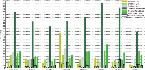
Examples of types of land disturbance and vegetation loss from 2005 to 2006 with the Landsat BAP scenes are shown in Figure 7(a–d). Area estimation of annual land disturbance types and pre-disturbed vegetation types including the contribution of oil and gas footprints from 2005 to 2013 are summarized in Figures 8 and 9, respectively. The highest amount of land disturbance was observed in 2008–2009 with 489 km² of vegetation loss, where 255 km² of vegetation was cleared (and attributed as bare soil), 179 km² of vegetation was turned into transitional bare surface, and 58 km² of vegetation was turned into developed and mixed developed footprints. Figure 8 shows that vegetation loss rate due to bare soil/cutblock and transitional bare surface disturbances was 293 km² per year, with 14% contribution from oil and gas footprints, and the vegetation loss rate due to developed and mixed developed disturbances was 89 km² per year, with 31% contribution from oil and gas footprints. Direct contribution of oil and gas footprints to the total amount of vegetation losses were usually less than 20% as shown in Figure 9. The highest amount of coniferous forest loss was observed with a rate of 178 km² per year based on the estimates shown in Figure 9, where 15% of the loss was directly related to oil and gas footprints and the rest were due to other anthropogenic and natural causes, e.g., wildfire and logging activities. In addition, broadleaf and mixed forest loss rate was 100 km² per year, and grassland, shrubland, and cropland loss rate was 104 km² per year.

Figure 7. False color composite (SWIR 1, NIR, Red) of (a) 2005 and (b) 2006 Landsat annual BAP data. (c) Types of land disturbances and (d) types of vegetation loss from 2005 to 2006.

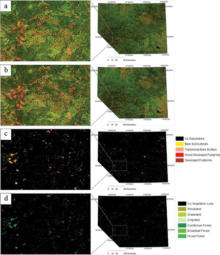
Figure 8. Area estimation of types of land disturbance from 2005 to 2013 including the contribution of oil and gas footprints.

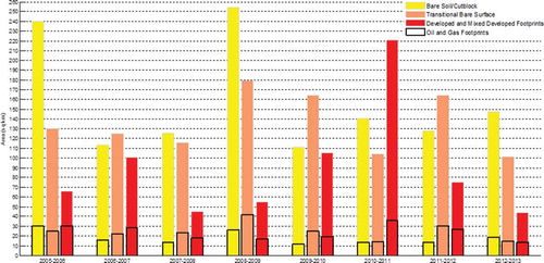
Figure 9. Area estimation of types of vegetation loss from 2005 to 2013 including the contribution of oil and gas footprints.

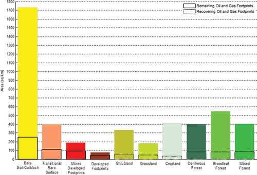
Figure 10(a) illustrates a cumulative land disturbance map from 2005 to 2013, which was utilized to assess the sign of vegetation recovery in cumulative land disturbances including oil and gas footprints in 2013 as illustrated in Figure 10(B–C). Figure 11 summarizes the result of Figure 10(a–c) with an estimated area of each type of remaining and recovering disturbances in 2013 out of 2005–2013 cumulative disturbances including oil and gas footprints. Remaining disturbances include 1730 km² of bare soil/cutblock, 389 km² of transitional bare surface, and 267 km² of developed and mixed developed footprints, where 21% of all remaining disturbances were oil and gas footprints. Recovering disturbances include 927 km² of shrubland, grassland, and cropland and 1353 km² of coniferous, mixed, and broadleaf forest, where 17% of all recoveries occurred within oil and gas footprints and approximately 44% of oil and gas disturbances from 2005 to 2013 were showing evidence of recovery.

Figure 10. (a) Cumulative land disturbances from 2005 to 2013 and (b) the state of cumulative land disturbances including (c) oil and gas footprints in 2013 with remaining disturbances and evidence of vegetation recovery.

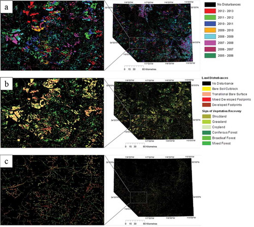
Figure 11. Area estimation of recovering and remaining disturbances in 2013 out of 2005–2013 cumulative land disturbances with the contribution of oil and gas footprints.

Validation

Accuracy assessment results of cumulative land disturbance from 2005 to 2013 are shown in Table 1 that indicates 87% overall accuracy with more than 80% producer accuracy for each year. Accuracy assessment results of the fused classification maps from 2005 to 2013 are summarized in Figure 12(a,b), where 78% average overall accuracy was observed for each year. Classes considered for accuracy assessment include developed and mixed developed footprint, shrubland, grassland, cropland, coniferous forest, and broadleaf forest. For accuracy assessment, developed footprints and mixed developed footprints were combined into the developed class. In addition, grassland and shrubland classes were combined into the shrub/grass class. High producer accuracy of usually more than 80% was observed for the developed, coniferous, and broadleaf classes as shown in Figure 12(a). However, low producer accuracy of usually less than 60% was observed for shrub/grass and cropland that could be associated with poor spectral separability of training data. An example of spectral library (training data) from 2009 is shown in Figure 13, and Table 2 shows the spectral separability of class pairs from 2009 based on the Jeffries-Matusita measure (Jeffreys 1946; Richards 1999), where lower values (i.e., less than 1.0) indicate poor separability that causes misclassification between classes, e.g., poor separability was observed between shrub/grass and cropland as well as shrub/grass and broadleaf. Table 3 shows an example of error matrix of 2013 LULC classification map with an overall accuracy of 77.49% with more than 75% producer accuracy for all classes except shrub/grass (30%), where ~50% shrub/grass was misclassified as broadleaf forest.

Table 1. Error matrix of cumulative land disturbances from 2005 to 2013.

Overall accuracy = (1,769,681/2,034,218) 87.00% Kappa coefficient = 0.8510
Class	2012–2013	2011–2012	2010–2011	2009–2010	2008–2009	2007–2008	2006–2007	2005–2006	Total
Ground reference (pixels)
2012–2013	187,691	14,168	511	390	531	776	658	1819	206,544
2011–2012	1838	252,750	20,674	2245	2454	1622	2085	4197	287,865
2010–2011	3211	10,635	266,844	6126	2100	2241	2875	5750	299,782
2009–2010	954	3565	18,710	22,1878	12,071	1189	1696	3359	263,422
2008–2009	1611	4866	3961	8413	224,847	12,345	2860	8388	267,291
2007–2008	413	1990	1838	1604	10,688	183,286	14,809	3250	217,878
2006–2007	2278	2859	3462	2731	3246	3003	193,537	21,404	232,520
2005–2006	1079	2284	2337	2159	4776	2448	4985	238,848	258,916
Total	199,075	293,117	318,337	245,546	260,713	206,910	223,505	287,015	2,034,218
Ground reference (%)
2012–2013	94.28	4.83	0.16	0.16	0.2	0.38	0.29	0.63	10.15
2011–2012	0.92	86.23	6.49	0.91	0.94	0.78	0.93	1.46	14.15
2010–2011	1.61	3.63	83.82	2.49	0.81	1.08	1.29	2	14.74
2009–2010	0.48	1.22	5.88	90.36	4.63	0.57	0.76	1.17	12.95
2008–2009	0.81	1.66	1.24	3.43	86.24	5.97	1.28	2.92	13.14
2007–2008	0.21	0.68	0.58	0.65	4.1	88.58	6.63	1.13	10.71
2006–2007	1.14	0.98	1.09	1.11	1.25	1.45	86.59	7.46	11.43
2005–2006	0.54	0.78	0.73	0.88	1.83	1.18	2.23	83.22	12.73
Total	100	100	100	100	100	100	100	100	100

Note: Bold values indicate producer accuracy.

Table 2. Jeffries-Matusita spectral separability measure ranked from least to most for pairs of selected training data from 2009.

Class pair		Least to most separability
Shrub/grass (847,087 pixels)	Cropland (209,676 pixels)	0.74
Shrub/grass (847,087 pixels)	Broadleaf (1,225,529 pixels)	0.94
Coniferous (1,729,107 pixels)	Broadleaf (1,225,529 pixels)	1.02
Shrub/grass (847,087 pixels)	Coniferous (1,729,107 pixels)	1.18
Developed (11,867 pixels)	Cropland (209,676 pixels)	1.39
Developed (11,867 pixels)	Shrub/grass (847,087 pixels)	1.49
Cropland (209,676 pixels)	Broadleaf (1,225,529 pixels)	1.59
Cropland (209,676 pixels)	Coniferous (1,729,107 pixels)	1.84
Developed (11,867 pixels)	Coniferous (1,729,107 pixels)	1.86
Developed (11,867 pixels)	Broadleaf (1,225,529 pixels)	1.87

Table 3. Error matrix of the 2009 LULC classification map.

Overall accuracy = (2,300,423/2,916,113) 78.89 % Kappa coefficient = 0.6805
Class	Developed	Shrub/grass	Cropland	Coniferous	Broadleaf	Total
Ground reference (pixels)
Developed	58,028	2931	8546	3525	2004	75,034
Shrub/grass	1599	120,511	9660	45,335	68,275	245,380
Cropland	199	27,935	101,420	4643	27,388	161,585
Coniferous	0	48,600	497	1,154,656	81,802	1,285,555
Broadleaf	2	197,834	15,084	56,161	639,547	908,628
Total	59,828	397,858	135,222	1,264,443	819,188	2,676,539
Ground reference (%)
Developed	96.99	0.74	6.32	0.28	0.24	2.8
Shrub/grass	2.67	30.29	7.14	3.59	8.33	9.17
Cropland	0.33	7.02	75.00	0.37	3.34	6.04
Coniferous	0	12.22	0.37	91.32	9.99	48.03
Broadleaf	0	49.72	11.15	4.44	78.07	33.95
Total	100	100	100	100	100	100

Note: Bold values indicate producer accuracy.

Figure 12. (a) Producer’s accuracy and (b) overall accuracy of annual LULC classification map from 2005 to 2013.

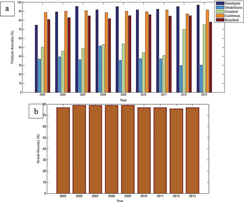
Figure 13. An example of spectral signatures of training data for 2009.

Limitations

In this study, LULC classification map for each target year (2005–2013) was produced based on the unchanged portion of training data from 2010 to each target year. The accuracy of selected training data, which includes a land-cover classification from 2010, influences the accuracy of annual LULC classification results (Castilla et al. 2014; Alberta Biodiversity Monitoring Institute 2015). Ground-reference data need to be collected to validate the results of cutblock/bare soil and mixed forest classes. Low producer accuracy (<50%) was observed for grass/shrub class that requires selection of better training data. The completeness of early release annual Landsat BAP data, i.e., “missing pixels” due to cloud cover, shadow, and noise, influences the quantitative extraction of year-to-year land disturbances (White et al. 2014). Initial stage of forest recovery was observed in the 9-year period, where a complete forest recovery can take up to 20 years depending on the severity of disturbances and reclamation performance of oil and gas footprints (Powers et al. 2015; Osko and MacFarlane 2001; Schneider 2002). Most of the oil and gas footprints (e.g., well pad, access road, and pipeline corridor) appear in Landsat imagery and are usually underestimated due to limited spatial resolution in relation to the size of the objects of interest. Fine-scale land disturbance estimates from higher spatial resolution time-series imagery (e.g., SPOT) can be 1.28 times greater than the one from Landsat time-series imagery (Komers and Stanojevic 2013). Inactive, abandoned, and infrequently used footprints might have substantial amount of spectral signature variability due to several factors, including: pervious/impervious surface types, short vegetation cover, and deep shadow from surrounding trees. These factors can lead to misclassification of disturbance and recovery including area estimation errors.

Conclusions

This study demonstrates the utilization of Landsat annual BAP composites of multispectral data to classify annual land disturbances, detect vegetation loss, and quantify the nature of vegetation recovery from 2005 to 2013. A fused LULC classification method based on the CEM, SAM, and ML algorithms was introduced with detailed extraction of developed and mixed developed industrial footprints as well as bare soil and vegetation classes. Contributions of oil and gas footprints to annual land disturbances were assessed with the DIDs geospatial data. The highest rate of observed vegetation loss (293 km² per year) was due to bare soil/cutblock and transitional bare surface disturbances compared to developed and mixed developed disturbances (89 km² per year). In addition, the highest rate of observed vegetation loss was observed for coniferous forest (178 km² per year) followed by loss of broadleaf/mixed forest (100 km² per year) and grassland/shrubland/cropland (104 km² per year). Less than 20% annual vegetation loss was directly related to oil and gas footprints, where the remaining vegetation loss could be related to logging activities, insect defoliation, wildfire, and harvesting of agricultural crops. In 2013, the recovering portion of 2005–2013 cumulative land disturbances includes 927 km² of shrubland, grassland, and cropland and 1352 km² of coniferous, broadleaf, and mixed forest, where remaining disturbances include 2119 km² of bare soil/cutblock and 267 km² of developed and mixed developed footprints. In addition, signs of recovery were observed in 44% of total oil and gas footprints. This type of study helps the energy regulator to develop realistic land-use planning tools that consider the impact of oil and gas development with respect to an established threshold. The annual LULC classification maps and land disturbance maps obtained 78% (average) and 87% overall accuracy, respectively. Although it is possible to classify and quantify the types of land disturbance, vegetation loss, and vegetation recovery with Landsat multispectral data, identification of the cause of land disturbance requires integration of time-series geospatial data associated with burn scars, Mountain Pine Beetle infestation, logging activities, and other land disposition types from DIDs; this can help the government to implement an efficient and transparent land-use plan to support sustainable development.

Acknowledgments

This study was carried out at the Alberta Geological Survey, Alberta Energy Regulator under the Earth Observation (EO) project. Results from this study were published as geospatial data at http://www.ags.aer.ca/data-maps-models/digital-data (DIG 2015-0028 to DIG 2015-0093). The authors are indebted to the United States Geological Survey server (http://earthexplorer.usgs.gov/) for providing the Landsat data and are grateful to Ms Joanne White and Mr Geordie Hobart from the Natural Resources Canada/Pacific Forestry Centre for producing and sharing the Landsat Best-Available-Pixel composites. The authors would like to thank Ms Susan Ning Quio from the University of Saskatchewan, Mr Barry Fildes, Ms Joan Walters, Dr Matt Grobe, Mr Andrew Beaton, and Mr Dan Palombi from the Alberta Energy Regulator/Alberta Geological Survey, and Dr Darren Pouliot from the Natural Resources Canada/Canada Center for Remote Sensing for their support. In addition, the authors would like to thank anonymous reviewers for their constructive comments to improve the quality of the manuscript.

Disclosure statement

No potential conflict of interest was reported by the authors.

References

- Alberta Biodiversity Monitoring Institute. 2015. “Land Cover Map, Year 2010, ABMI Wall-To-Wall Land Cover Map.” Accessed 11 October 2015. http://www.abmi.ca/home/data/gis-data/land-cover-download.html
- Alberta Environment and Parks. 2015a. “Biophysical, Alberta Merged Wetland Inventory.” Accessed 26 October 2015. http://aep.alberta.ca/forms-maps-services/maps/resource-data-product-catalogue/biophysical.aspx
- Alberta Environment and Parks. 2015b. “Digital Integrated Dispositions.” Accessed 26 October 2015. http://aep.alberta.ca/lands-forests/land-management/digital-integrated-dispositions.aspx
- Arora, M. K., S. Bansal, S. Khare, and K. Chauhan. 2013. “Comparative Assessment of Some Target Detection Algorithms for Hyperspectral Images.” Defence Science Journal 63 (1): 53–62. doi:10.14429/dsj.63.3764.
- Atkinson, P. M., and A. R. L. Tatnall. 1997. “Introduction to Neural Networks in Remote Sensing.” International Journal of Remote Sensing 11: 699–709. doi:10.1080/014311697218700.
- Baiocchi, V., R. Brigane, D. Dominici, and F. Radicioni. 2012. “Coastline Detection Using High Resolution Multispectral Satellite Images.” Proceedings of the FIG Working Week 1–15.
- Baker, B. A., T. A. Warner, J. F. Conley, and B. E. McNeil. 2013. “Does Spatial Resolution Matter? A Multi-Scale Comparison of Object-Based and Pixel-Based Methods for Detecting Change Associated with Gas Well Drilling Operations.” International Journal of Remote Sensing 34 (5): 1633–1651. doi:10.1080/01431161.2012.724540.
- Boardman, J. W., F. A. Kruse, and R. O. Green. 1995. “Mapping Target Signatures via Partial Unmixing of AVIRIS Data.” In Summaries, Fifth JPL Airborne Earth Science Workshop, JPL Publication 95-1 (1): 23–26.
- Castilla, G., J. Hird, R. J. Hall, J. Schieck, and G. McDermid. 2014. “Completion and Updating of a Landsat-Based Land Cover Polygon Layer for Alberta, Canada.” Canadian Journal of Remote Sensing 40 (2): 92–109. doi:10.1080/07038992.2014.933073.
- Chang, C.-I., J.-M. Liu, B.-C. Chieu, C.-M. Wang, C. S. Lo, P.-C. Chung, H. Ren, C. ‑. W. Yang, and D.-J. Ma. 2000. “A Generalized Constrained Energy Minimization Approach to Subpixel Target Detection for Multispectral Imagery.” Optical Engineering 39 (5): 1275–1281. doi:10.1117/1.602486.
- Chen, X.-L., H.-M. Zhao, P.-X. Li, and Z.-Y. Yin. 2006. “Remote Sensing Image-Based Analysis of the Relationship between Urban Heat Island and Land Use/Cover Changes.” Remote Sensing of Environment 104 (2): 133–146. doi:10.1016/j.rse.2005.11.016.
- Du, Q., H. Ren, and C.-I. Chang. 2003. “A Comparative Study for Orthogonal Subspace Projection and Constrained Energy Minimization.” IEEE Transactions on Geoscience and Remote Sensing 41 (6): 1525–1529. doi:10.1109/tgrs.2003.813704.
- ERCB (Energy Resources Conservation Board). 2012. Regulating Unconventional Oils & Gas in Alberta. A Discussion Paper 31.
- EXELIS Visual Information Solutions. 2015. “SPEAR Lines of Communication (LOC) – Water, Supervised, Spectral Matching.” Accessed 19 October 2015. http://www.exelisvis.com/docs/SPEARLinesOfCommunicationWater.html
- Farrand, W.H., and J.C. Harsanyi. 1997. “Mapping The Distribution Of Mine Tailings In The Coeur D’alene River Valley, Idaho, Through The Use Of A Constrained Energy Minimization Technique.” Remote Sensing Of Environment 59: 64–76. doi:10.1016/S0034-4257(96)00080-6.
- Gillanders, S. N., N. C. Coops, M. A. Wulder, S. E. Gergel, and T. Nelson. 2008. “Multitemporal Remote Sensing of Landscape Dynamics and Pattern Change: Describing Natural and Anthropogenic Trends.” Progress in Physical Geography 32 (5): 503–528. doi:10.1177/0309133308098363.
- Government of Alberta. 2015. “Upper Peace Regional Plan (UPRP) and Upper Athabasca Regional Plan (UARP) Well Pad Footprint.” Accessed 14 October 2015. http://open.alberta.ca/opendata/uprpuarp-well-pad-footprint#summary
- Green, A. A., M. Berman, P. Switzer, and M. D. Craig. 1988. “A Transformation for Ordering Multispectral Data in Terms of Image Quality with Implications for Noise Removal.” IEEE Transactions on Geoscience and Remote Sensing 26 (1): 65–74. doi:10.1109/36.3001.
- Grekousis, G., G. Mountrakis, and M. Kavouras. 2015. “An Overview of 21 Global and 43 Regional Land-Cover Mapping Products.” International Journal of Remote Sensing 36 (21): 5309–5335. doi:10.1080/01431161.2015.1093195.
- Hagner, O., and H. Reese. 2007. “A Method for Calibrated Maximum Likelihood Classification of Forest Types.” Remote Sensing of Environment 110 (4): 438–444. doi:10.1016/j.rse.2006.08.017.
- Hansen, M., R. Dubayah, and Defries. 1996. “Classification Trees: An Alternative to Traditional Land Cover Classifiers.” International Journal of Remote Sensing 17 (5): 1075–1081. doi:10.1080/01431169608949069.
- Hansen, M. C., P. V. Potapov, R. Moore, M. Hancher, S. A. Turubanova, A. Tyukavina, D. Thau, et al. 2013. “High-Resolution Global Maps of 21st-Century Forest Cover Change.” Science. 342 (15 November): 850–853. Data available on-line from doi:10.1126/science.1244693
- Harsanyi, J. C., and C.-I. Chang. 1994. “Hyperspectral Image Classification and Dimensionality Reduction: An Orthogonal Subspace Projection Approach.” IEEE Transactions on Geoscience and Remote Sensing 32 (4): 779–785. doi:10.1109/36.298007.
- He, Y., S. Franklin, E. X. Guo, and G. B. Stenhouse. 2009. “Narrow-Linear and Small-Area Forest Disturbance Detection and Mapping from High Spatial Resolution Imagery.” Journal of Applied Remote Sensing 3 (1): 033570. doi:10.1117/1.3283905.
- Hobson, K. A., and E. Bayne. 2000. “Effects of Forest Fragmentation by Agriculture on Avian Communities in the Southern Boreal Mixedwoods of Western Canada.”.” The Wilson Bulletin 112 (3): 373–387. doi:10.1676/0043-5643(2000)112[0373:eoffba]2.0.co;2.
- Hussain, M., D. Chen, A. Cheng, H. Wei, and D. Stanley. 2013. “Change Detection from Remotely Sensed Images: From Pixel-Based to Object-Based Approaches.” ISPRS Journal of Photogrammetry and Remote Sensing 80: 91–106. doi:10.1016/j.isprsjprs.2013.03.006.
- Inc, E. 1999. Erdas Field Guide. Atlanta, Georgia: Erdas Inc..
- Jeffreys, H. 1946. “An Invariant for the Prior Probability in Estimation Problems.” Proceedings Roy Social A 186: 454–461. doi:10.1098/rspa.1946.0056.
- Jensen, J. R. 2004. “Introductory Digital Image Processing: A Remote Sensing Perspective.” In Upper Saddle River, 431–462. 3 ed. NJ: Pearson Education Inc.
- Ji, L., X. Geng, K. Sun, Y. Zhao, and P. Gong. 2015. “Target Detection Method for Water Mapping Using Landsat 8 OLI/TIRS Imagery.” Water 7 (2): 794–817. doi:10.3390/w7020794.
- Komers, P. E., and Z. Stanojevic. 2013. “Rates of Disturbance Vary by Data Resolution: Implications for Conservation Schedules Using the Alberta Boreal Forest as a Case Study.” Global Change Biology 19 (9): 2916–2928. doi:10.1111/gcb.12266.
- Kruse, F. A., A. B. Lefkoff, J. W. Boardman, K. B. Heidebrecht, A. T. Shapiro, P. J. Barloon, and A. F. H. Goetz. 1993. “The Spectral Image Processing System (SIPS) – Interactive Visualization and Analysis of Imaging Spectrometer Data.” Remote Sensing of Environment 44 (2–3): 145–163. doi:10.1016/0034-4257(93)90013-n.
- Linke, J., S. E. Franklin, F. Huettmann, and G. B. Stenhouse. 2005. “Seismic Cutlines, Changing Landscape Metrics and Grizzly Bear Landscape Use in Alberta.” Landscape Ecology 20 (7): 811–826. doi:10.1007/s10980-005-0066-4.
- Meddens, A. J., A. T. Hudak, J. S. Evans, W. A. Gould, and G. González. 2008. “Characterizing Forest Fragments in Boreal, Temperate, and Tropical Ecosystems.” AMBIO: A Journal of the Human Environment 37 (7): 569–576. doi:10.1579/0044-7447-37.7.569.
- Osko, T., and A. MacFarlane. 2001. “Natural Reforestation on Seismic Lines and Wellsites in Comparison to Natural Burns or Logged Sites.” In Alberta-Pacific Forest Industries. Boyle, Alberta. OSKO Natural Resource Consulting and University of Alberta for Alberta Pacific Forest Industries Inc.
- Otukei, J. R., and T. Blaschke. 2010. “Land Cover Change Assessment Using Decision Trees, Support Vector Machines and Maximum Likelihood Classification Algorithms.” International Journal of Applied Earth Observation and Geoinformation 12: S27–S31. doi:10.1016/j.jag.2009.11.002.
- Pal, M., and P. M. Mather. 2005. “Support Vector Machines for Classification in Remote Sensing.” International Journal of Remote Sensing 26 (5): 1007–1011. doi:10.1080/01431160512331314083.
- Pasher, J., E. Seed, and J. Duffe. 2013. “Development of Boreal Ecosystem Anthropogenic Disturbance Layers for Canada Based on 2008 to 2010 Landsat Imagery.” Canadian Journal of Remote Sensing 39 (1): 42–58. doi:10.5589/m13-007.
- Potapov, P., S. Turubanova, and M. C. Hansen. 2011. “Regional-Scale Boreal Forest Cover and Change Mapping Using Landsat Data Composites for European Russia.” Remote Sensing of Environment 115 (2): 548–561. doi:10.1016/j.rse.2010.10.001.
- Pouliot, D., and R. Latifovic. 2016. “Land Change Attribution Based on Landsat Time Series and Integration of Ancillary Disturbance Data in the Athabasca Oil Sands Region of Canada.” Giscience & Remote Sensing 53 (3): 382–401. doi:10.1080/15481603.2015.1137112.
- Powers, R. P., T. Hermosilla, N. C. Coops, and G. Chen. 2015. “Remote Sensing and Object-Based Techniques for Mapping Fine-Scale Industrial Disturbances.” International Journal of Applied Earth Observation and Geoinformation 34: 51–57. doi:10.1016/j.jag.2014.06.015.
- Richards, J. A. 1999. Remote Sensing Digital Image Analysis, 240. Berlin: Springer-Verlag.
- Salehi, B., Z. Chen, W. Jefferies, P. Adlakha, P. Bobby, and D. Power. 2014. “Well Site Extraction from Landsat-5 TM Imagery Using an Object- and Pixel-Based Image Analysis Method.” International Journal of Remote Sensing 35 (23): 7941–7958. doi:10.1080/01431161.2014.978042.
- Schneider, R. R. 2002. Alternative Futures. Alberta’s Boreal Forest at the Crossroads. Edmonton: The Federation of Alberta Naturalists and the Alberta Centre for Boreal Research.
- Schroeder, T. A., M. A. Wulder, S. P. Healey, and G. G. Moisen. 2011. “Mapping Wildfire and Clearcut Harvest Disturbances in Boreal Forests with Landsat Time Series Data.” Remote Sensing of Environment 115 (6): 1421–1433. doi:10.1016/j.rse.2011.01.022.
- Shafri, H. Z., A. Suhaili, and S. Mansor. 2007. “The Performance of Maximum Likelihood, Spectral Angle Mapper, Neural Network and Decision Tree Classifiers in Hyperspectral Image Analysis.” Journal of Computer Science 3 (6): 419–423. doi:10.3844/jcssp.2007.419.423.
- Staenz, K., J. Schwarz, L. Vernaccini, F. Vachon, and C. Nadeau. 1999. “Classification of Hyperspectral Agricultural Data with Spectral Matching Techniques.” Proceedings of the International Symposium on Spectral Sensing Research, Las Vegas, Nevada 12–20.
- Sun, J., J. Yang, C. Zhang, W. Yun, and J. Qu. 2013. “Automatic Remotely Sensed Image Classification in a Grid Environment Based on the Maximum Likelihood Method.” Mathematical and Computer Modelling 58 (3–4): 573–581. doi:10.1016/j.mcm.2011.10.063.
- Tou, J. T., and R. C. Gonzalez. 1974. Pattern Recognition Principles. Reading, Massachusetts: Addison-Wesley Publishing Company.
- Waske, B., and J. A. Benediktsson. 2007. “Fusion of Support Vector Machines for Classification of Multisensor Data.” IEEE Transactions on Geoscience and Remote Sensing 45 (12): 3858–3866. doi:10.1109/tgrs.2007.898446.
- White, J. C., M. A. Wulder, G. W. Hobart, J. E. Luther, T. Hermosilla, P. Griffiths, N. C. Coops, et al. 2014. “Pixel-Based Image Compositing for Large-Area Dense Time Series Applications and Science.” Canadian Journal of Remote Sensing 40 (3): 192–212. doi:10.1080/07038992.2014.945827.
- Zha, Y., J. Gao, and S. Ni. 2003. “Use of Normalized Difference Built-Up Index in Automatically Mapping Urban Areas from TM Imagery.” International Journal of Remote Sensing 24 (3): 583−594. doi:10.1080/01431160304987.
- Zhang, Y., B. Guindon, N. Lantz, T. Shipman, D. Chao, and D. Raymond. 2014. “Quantification of Anthropogenic and Natural Changes in Oil Sands Mining Infrastructure Land Based on Rapideye and SPOT5.” International Journal of Applied Earth Observation and Geoinformation 29: 31–43. doi:10.1016/j.jag.2013.11.013.