Using low-density discrete Airborne Laser Scanning data to assess the potential carbon dioxide emission in case of a fire event in a Mediterranean pine forest

Abstract

The aim of study is to map the carbon dioxide (CO₂) emission of the aboveground tree biomass (AGB) in case of a fire event. The suitability of low point density, discrete, multiple-return, Airborne Laser Scanning (ALS) data and the influence of several characteristics of these data and the study area on the results obtained have been evaluated. A sample of 45 circular plots representative of Pinus halepensis Miller stands were used to fit and validate the model of AGB. The ALS point clouds were processed to obtain the independent variables and a multivariate linear regression analysis between field data and ALS-derived variables allowed estimation of AGB. Then, the influence of several characteristics on the residuals of the model was analyzed. Finally, conversion factors were applied to obtain the CO₂ values. The AGB model presented a R² value of 0.84 with a relative root-mean-square error of 27.35%. This model included ALS variables related to vegetation height variability and to canopy density. Terrain slope, aspect, canopy cover, scan angle and the number of laser returns did not influence AGB estimations at plot level.

Keywords:

• LiDAR
• area-based approach
• biomass
• Pinus halepensis Miller

1. Introduction

Forest ecosystems play an important role in the global carbon cycle, since carbon is exchanged naturally between forests and the atmosphere through photosynthesis, decomposition and combustion (García et al. 2010). Biomass carbon pools act as a sink for atmospheric carbon dioxide (CO₂). However, forest fires are a critical factor because the carbon stored during photosynthesis is released into the atmosphere contributing to greenhouse gas emissions (Chuvieco 2009). According to the Spanish Official Report to the United Nations Framework Convention on Climate Change (1990–2013), the CO₂ emissions into the atmosphere by forest fires occurred in the Spanish territory since 1990 are estimated in an annual average of 1.45 million tons, implying the destruction of the green cover and the loss of a major carbon sink.

The CO₂ emissions are estimated from carbon contained in the biomass above the ground (Chuvieco 2009; Carvalho et al. 2016). In this context, accurate and spatially explicit estimates of forest biomass are required for the following reasons: (1) to increase the understanding of the contribution of forests to the carbon cycle, (2) to support national policies focused on preserve carbon stock and to reduce emissions (Muukkonen and Heiskanen 2007; Mieville et al. 2010; Pan et al. 2011), (3) to achieve sustainable silvicultural treatments, (4) to estimate fuel loading and (5) to assess the available resources for bioenergy production (Montero, Ruiz-Peinado, and Muñoz 2005; García et al. 2010).

Conventional methods for biomass estimation are based on direct field measurements commonly limited in terms of spatial and temporal samplings because they require extensive destructive measurements. Alternatively, remote sensing techniques provide information at a wide range of spatial and temporal scales on forest biomass (Rosette et al. 2012). Numerous studies have correlated the ground-measured biomass data and the spectral response of vegetation cover using passive optical imagery to estimate biomass (e.g. Foody, Boyd, and Cutler 2003; Leboeuf et al. 2007; Meng et al. 2007; Muukkonen and Heiskanen 2007; García-Martín et al. 2008; García-Martín et al. 2012; Liu et al. 2015). The results can be affected by saturation problems, especially when the vegetation is in the growing season, and the Normalized Difference Vegetation Index (NDVI) may fail to correctly response the vegetation status. This is very noticeable when the aboveground biomass is higher than 100 ton/ha (Lu 2006; García et al. 2010). However, for other vegetation indexes, e.g. Ratio Vegetation Index, Leaf Area Index, the saturation problems are not as serious as the NDVI. Synthetic Aperture Radar (SAR) data have been shown a higher sensitivity to greater amounts of biomass, although the results are variable depending on the band selected and the environmental conditions of the study area (Lu 2006; Tanase et al. 2014). Light Detection and Ranging (LiDAR) is becoming one of the most accurate techniques in forest attribute estimation (Maltamo, Næsset, and Vauhkonen 2014; Vosselman and Maas 2010) given the capability of LiDAR sensors to provide 3-D information of vegetation structure although it remains expensive compared to satellite-based remote sensing technologies.

One of the most commonly used LiDAR systems are small-footprint, discrete-return airborne lasers, also referred to as Airborne Laser Scanning (ALS), which has shown great potential to estimate biomass using different approaches (i.e. Koch 2010; Vosselman and Maas 2010; Zolkos, Goetz, and Dubayah 2013; Maltamo, Næsset, and Vauhkonen 2014). Discrete-return systems have been used to successfully estimate aboveground biomass at individual tree level and at forest stand level (Lim and Treitz 2004; Bortolot and Wynne 2005; Popescu 2007; Næsset and Gobakken 2008). For tree-level inventories, ALS data are used to detect individual treetops and to predict attributes using sets of allometric models, providing estimates with a higher spatial resolution (Vauhkonen et al. 2012; Sačkov et al. 2016). In contrast, in the area-based approach (ABA), the heights corresponding to all the returns for a given surface area, for example a sample plot, are used to characterize the ground surface and the vertical distribution of the biological material (Maltamo, Næsset, and Vauhkonen 2014). In general, estimation of aboveground tree biomass (AGB) is based on regression equations relating vegetation biomass to a pool of potential ALS-derived variables from returns at plot level (Bouvier et al. 2015). These approaches mainly use point density ALS data above 1 point/m² and are applied to homogeneous boreal forest. Other studies have also shown the potential of ALS systems to estimate forest carbon content using several approaches, such as a quantile-based methodology in deciduous forests in the UK (Patenaude et al. 2004), by combining ALS data and environmental conditions that influence the ecosystem (Thomas et al. 2008), using intensity information (García et al. 2010), or by means of high-resolution ALS data (Lee, Kim, and Choi 2013). However, little research has been performed on the estimation of CO₂ emissions, especially when several European countries such as The Netherlands, Norway, Austria, Switzerland, Finland and Spain have partial or complete nationwide coverages of ALS data (Rosette et al. 2012). Point clouds derived from such national campaigns generally have low point density in order to reduce costs. Research indicates that the point density required to implement the ABA can be as low as 0.5 points/m² in some forest environments (Treitz et al. 2012). For example, Jakubowski, Guo, and Kelly (2013) show that correlations between metrics such as tree height or total basal area are relatively unaffected until pulse density drops below 1 return per square meter.

Despite not being intended for vegetation applications, these nationwide LiDAR datasets can be exploited for biomass mapping at regional scale, and consequently to estimate CO₂ (Rosette et al. 2012). This can be an alternative approach to burned area and the fuel load estimation with satellite data, calculating thereafter the combustion efficiency using the appropriate emission factors for the gas (Saranya, Sudhakar Reddy, and Prasada Rao 2016).

Pinus halepensis Miller (P. halepensis) is the most relevant tree species in the western Mediterranean Basin, where it is dominant in the semiarid areas (Gazol et al. 2017). Particularly, in the Spanish Region of Aragón, the P. halepensis is the most important tree species (Bujarrabal 2009). Although P. halepensis forests are well adapted to fire due to its high postfire seeding capacity (Moya et al. 2008; Chuvieco 2009; Fournier et al. 2013), they are affected yearly by wild and man-induced fires, being the major environmental damage in the Mediterranean regions (Moriondo et al. 2006; Battipaglia et al. 2014). The main problem is the high fire severity registered and the fire recurrence, which can affect the regeneration process (Pausas et al. 2008) and reduce the carbon sequestration.

Considering all the aforementioned data, the main aim of this study is to estimate the potential release of CO₂ after a hypothetic case of wildfire event in P. halepensis stands located in the Aragón Region. An empirical AGB model will be developed using low-density discrete ALS data and in situ measurements. The specific objectives are (1) to develop a multiple regression analysis for the aboveground biomass; (2) to analyze the effect of terrain slope, aspect, canopy cover, quantity of laser returns and scan angle on the residuals of the model; and (3) to map the AGB and the CO₂ emissions. This study contributes to clarify the relationship between AGB and wildfires in Mediterranean forest stands, providing a tool to analyze CO₂ emissions in a regular scenario in Spain.

2. Materials and methods

2.1. Study area

The P. halepensis forests under study are located in the Middle Ebro Basin, in northeastern Spain (41°50ʹ N, 0º57ʹ W). Climate is Mediterranean with continental features (Vicente-Serrano, Lasanta, and Gracia 2010).

The P. halepensis forests occupy 8266 ha (Figure 1). This species commonly occupies the top and slopes in the structural platforms of Miocene carbonate and marl sediments at about 750 m.a.s.l. (meters above sea level) (Vicente-Serrano, Lasanta, and Gracia 2010). Most of them are natural, but some stands, particularly the ones located in the south-eastern part of the study area at about 300 m.a.s.l., were planted approximately 40 years ago. The understory is dominated by evergreen shrubs, such as Quercus coccifera L., Juniperus oxycedrus L. subsp. macrocarpa (Sibth. & Sm.) Ball, Thymus vulgaris L. and Rosmarinus officinalis L.

Figure 1. Land cover types of the study area and locations of 45 forest inventory plots.

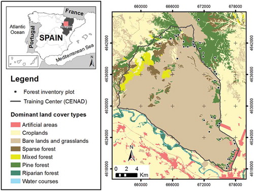
Part of the study area is located inside the Military Training Center (CENAD) “San Gregorio”, involving a direct risk of fire (Figure 1). These forest stands, characteristic of Mediterranean ecosystems, are subject to frequent wildfires. The most important wildfire burned 2,200 ha with a high severity in 2008 (Tanase, De La Riva, and Pérez-Cabello 2011), which is located in the north part of the study area (Figure 1).

2.2. ALS data

The ALS data were provided by the Spanish National Plan for Aerial Orthophotography (PNOA, http://www.ign.es/PNOA/vuelo_lidar.html) and recorded between 23 January and 2 February 2011 using a small-footprint airborne Leica ALS60 discrete return sensor. Data were delivered unclassified with up to four returns recorded per pulse. The sensor was operated at a wavelength of 1.064 μm and a scan angle of ±29º from nadir. The point density was 1 point/m² and the vertical accuracy was better than 0.20 m.

First, the noise of the point cloud was cleaned using the open-source BCAL LiDAR module, developed by Idaho State University, Boise Center Aerospace Laboratory (BCAL). Then, a filtering process was performed to identify ground returns. The classification algorithm implemented in the MCC software 2.1, developed by Evans and Hudak (2007), was applied given its good performance in hilly forest landscapes. The points classified as bare ground were interpolated using the “Point-TIN-Raster” interpolation method (Renslow 2013) in ArcGIS 10.2 software (ESRI, Redlands, CA, USA) to create a 1 m spatial resolution digital elevation model (DEM) (Montealegre, Lamelas, and De La Riva 2015). In order to obtain the aboveground heights, i.e. the normalized heights of the points, the ground elevation value of the DEM was subtracted from the ALS point height using FUSION LDV 3.30 open-source software (McGaughey 2009). Finally, a full suite of statistical metrics commonly used as independent variables in vegetation modeling (Evans et al. 2009) was generated with the “CloudMetrics” command. Following Nilsson (1996) and Naesset and Okland (2002), ALS-derived metrics were calculated applying a threshold value of 1 m height in order to exclude the returns belonging to bare-earth and understory.

2.3. Field data

Field data were obtained in 45 plots and served as ground reference in order to adjust and validate the predictive model of AGB. First, the central points of the field plots were selected using a stratified random sampling technique to ensure that the locations cover the range of terrain slopes and canopy cover of the study area (Naesset and Okland 2002). The terrain slope map was derived from the DEM generated previously and the canopy cover map was calculated as the percentage of first returns above 1 m height on total number of first returns. The bin size was 10 m. As can be seen in Table 1, the terrain slope average for selected plots was 10.7° and ranged from 0.7° to 25.7°. The canopy cover mean value for plots was 62.9 % and ranged from 16.1% to 93.0%.

Table 1. Summary of the field plot data (n = 45).

Variable	Min	Max	Range	Mean	Standard deviation
Elevation (m)	246.7	722.5	475.9	467.9	156.7
Terrain slope (degrees)	0.7	25.7	25.0	10.7	7.3
Canopy cover (%)	16.1	93.0	76.8	62.9	19.2
Tree height (m)	3.7	11.3	7.6	7.1	2.0
dbh: breast height diameter (cm)	8.6	28.3	19.7	15.2	4.7
AGB: aboveground biomass (ton/ha)	1.0	112.1	111.1	37.5	27.9
Wr: belowground biomass (ton/ha)	0.4	32.7	32.3	13.2	7.4
TB: total biomass (ton/ha)	1.4	144.8	143.4	50.7	35.1

Field data were collected from July to September 2014. The centroids of each circular plot (15 m radius) were located in the field using a Leica VIVA® GS15 CS10 GNSS real-time kinematic Global Positioning System, achieving an average planimetric accuracy of 0.15 m.

The total tree height (h) was measured using a Vertex instrument (Haglöf Sweden®). Tree diameters were calculated as breast height diameter (dbh), at the Europe standard height of 1.3 m, using a Mantax Precision Blue diameter caliper (Haglöf Sweden®). Only the trees with a dbh >7.5 cm were inventoried in each plot. Trees inventoried varied in height from 3.7 to 11.2 m and had dbh from 8.5 to 28.3 cm (Table 1).

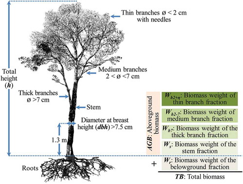
In order to estimate AGB at plot level, first the different biomass fractions were calculated at tree level, using the P. halepensis allometric models reported by Ruiz-Peinado, Del Rio, and Montero (2011) (Equations (1)–(4)):

(1) $W_{\mathrm{s}}\left(\mathrm{k}\mathrm{g}\right)=0.0139\times db{h}^2\times h\dots \dots \dots .$(1)

(2) $\begin{array}{c}{W}_{\text{b7}}\left(\text{kg}\right)=\left[\text{3}.\text{926}\times \left(dbh\text{-27}.\text{5}\right)\right]\times Z;\text{If}dbh\\ \le \text{27}.\text{5}\text{cm}\text{then}Z\text{=0};\text{If}dbh>\text{27}.\text{5cm}\text{then}Z=1\end{array}$(2)

(3) $W_{\mathrm{b}2-7}{\left(\mathrm{k}\mathrm{g}\right)}_{ }=4.257+0.00506\times \mathrm{d}\mathrm{b}{\mathrm{h}}^2\times h-0.0722\times \mathrm{d}\mathrm{b}\mathrm{h}\times h$(3)

(4) $W_{\mathrm{b}2+n}{\left(\mathrm{k}\mathrm{g}\right)}_{ }=6.197+0.00932\times db{h}^2\times h-0.0686\times dbh\times h$(4)

where W_s is the biomass weight of the stem fraction, W_b7 is the biomass weight of the thick branch fraction (diameter larger than 7 cm), W_b2 - ₇ is the biomass weight of medium branch fraction (diameter between 2 and 7 cm), and W_b2 + n is the biomass weight of thin branch fraction (diameter smaller than 2 cm) with needles (see Figure 2).

Figure 2. P. halepensis morphology and the tree biomass fractions according to Ruiz-Peinado, Del Rio, and Montero (2011). The total biomass (TB) refers to the dry weight of the plant material from trees, including roots, stems, bark, branches and leaves from the ground to the apex. The biomass of a tree can be divided into fractions above- and belowground (Maltamo, Næsset, and Vauhkonen 2014).

Then, the AGB of each tree was calculated summing up the biomass fractions obtained from Equations (1) to (4). Afterwards, the AGB values from each tree in every plot were summed up to obtain unique values per plot. Finally, the plot values were expressed in tons of dry biomass per hectare. Table 1 presents the minimum, maximum, range, mean and standard deviation values of different biomass fractions for the field plots. The AGB ranged from 1.0 and 112.1 ton/ha, with a mean value of 37.5 ton/ha.

2.4. Predictive model for estimating AGB

2.4.1. Selection of ALS metrics

Following Means et al. (2000), Naesset (2002), Gonzalez-Ferreiro, Dieguez-Aranda, and Miranda (2012), García, Godino, and Mauro (2012) and Watt et al. (2013), a multivariate linear regression approach was adopted in order to develop a model able to estimate the AGB. Given the large number of potential ALS-derived metrics, the Spearman’s rank correlation coefficient (Rho) was first applied in order to select those independent variables with the strongest correlation coefficient with the AGB (Watt et al. 2013). A minimum Rho value of ±0.50 was selected as a threshold to select the ALS-metrics.

2.4.2. Establishment of the model

The selected variables were included in a forward stepwise regression, trying to develop a parsimonious model in order to avoid over-fitting (Hair et al. 1999; Andersen, McGaughey, and Reutebuch 2005; Chen et al. 2007; González-Olabarria et al. 2012; Maltamo, Næsset, and Vauhkonen 2014). Predictor variables with a significance value of partial F statistic greater than 0.05 were removed from the model (Naesset and Okland 2002). The statistical assumptions of linearity, normality of the residuals, homoscedasticity, and independence or no autocorrelation were also verified (Hair et al. 1999; García, Godino, and Mauro 2012).

2.4.3. Model validation

A leave-one-out cross-validation (LOOCV) technique was applied with the purpose of performing an unbiased assessment of the predictive capacity of the regression model (Naesset and Okland 2002; Andersen, McGaughey, and Reutebuch 2005; Bouvier et al. 2015).

The predictive value of the model was assessed comparing the adjusted coefficient of determination (R²), which is the fraction of variance that is explained by the model. In addition, the root-mean-square error (RMSE) and relative root-mean-square error (%RMSE) were compared against the root-mean-square error for cross-validation (RMSEcv) and the relative root-mean square error for cross-validation (%RMSEcv), respectively. The RMSE gives an idea of the precision estimates in the same units as the dependent variable. A close agreement between RMSEcv and RMSE indicates that the regression model is not overfitting the data and presents a good predictive value. Finally, the mean of the residuals (bias) was also obtained using the LOOCV technique (Andersen, McGaughey, and Reutebuch 2005).

2.5. Error analysis of the AGB estimation

In order to gain a better understanding of the error introduced in the AGB predictions by factors related to topography, forest structure and ALS data, a statistical analysis was performed. Residuals derived from the AGB model at each sample plot were categorized across a range of values of each factor considered: terrain slope, aspect, canopy cover, quantity of laser returns and scan angle (see Table 2).

Table 2. Ranges applied to the variables influencing the accuracy of the estimations.

Variable	Source	Categories	Number of plots
Terrain slope (degrees)	ALS-derived DEM	Gentle (0–5)	11
		Moderate (5–15)	25
		Steep slopes (>15)	9
Aspect (degrees)	ALS-derived DEM	Indifferent (−1–0; 67.5–90; 247.5–270)	5
		Shady (0–67.5; 270–360)	19
		Sunny (90–247.5)	21
Canopy cover (%)	ALS data	Low (<40)	7
		Medium (40–70)	18
		High (>70)	20
Quantity of laser returns(number of points)	ALS data	Low (0–300)	9
		Medium (300–800)	21
		High (>800)	15
Scan angle (degrees)	ALS data	Low (0–±5)	23
		Medium (±5–±10)	10
		High (>±10)	12

Slope and canopy cover have been considered as these variables influence the accuracy of DEMs developed from ALS data according to Clark, Clark, and Roberts (2004) and Kraus and Pfeifer (1998). Consequently they could affect the accuracy of derived forest height metrics (Renslow 2013).

Aspect is closely related to insolation and, as a consequence, to moisture presence, affecting ultimately to vegetation development. In fact, in the study area, the pine forest located on south-facing slopes presents less dense structure than the one located on north-facing slopes.

The canopy cover can influence the vertical interception of laser hits (Renslow 2013). Furthermore, in a scenario of sparse density of returns, some trees cannot be detected. This may lead to an underestimation of the average stand height, as some tree tops are missed (Vosselman and Maas 2010). According to Goodwin, Coops, and Culvenor (2006), the amount of returns available has been shown to be even more important than footprint size or flight altitude in determining forest variables, such as crown area and volume.

Scan angle was also considered in the analysis as, according to Gatziolis and Andersen (2008) and Holmgren, Nilsson, and Olsson (2003), in dense forest stands, if scan angles exceed 12–14º, often artefacts occur due to multipath errors. These artefacts can produce a bias in forest structure attributes estimation. It should be noted that the ALS data provided by the PNOA mission do not discard those returns higher than 14º, so it is interesting to analyse if it is necessary to remove these points with high scan angles in future approaches.

A Kruskal–Wallis test was used to compare the medians among categories of the variables (Table 2). This nonparametric test is useful when it is impossible to assume the normality of the sample.

2.6. Carbon dioxide emissions mapping

The pixel size selected to compute the ALS-derived metrics was 25 m × 25 m, representing an area of 625 m², which approximates the field plot dimensions. Metrics included in the AGB model equation were transformed into raster layers using the “GridMetrics” and “CSV2Grid” commands implemented in FUSION LDV 3.30 (McGaughey 2009). Finally, Equation (5) was applied to quantify the release of CO_2, assuming a hypothetical scenario of high fire severity in which all of the aerial parts of the trees would be consumed.

(5) $\mathrm{C}{\mathrm{O}}_2=\mathrm{A}\mathrm{G}\mathrm{B}\times 0.499\times 3.67\times 0.888$(5)

where AGB is the aboveground tree biomass, 0.499 is a conversion factor for the P. halepensis to obtain the carbon content according to Montero, Ruiz-Peinado, and Muñoz (2005), 3.67 is an emission factor applied to convert carbon into CO₂ (Montero, Ruiz-Peinado, and Muñoz 2005) and 0.888 is the proportion of CO₂ emitted into the atmosphere according to Trozzi, Vaccaro, and Piscitello (2002).

3. Results

3.1. The AGB model

Table 3 shows the Spearman’s rank correlation coefficients between plot-derived AGB and ALS-derived metrics, respectively. The AGB presents a direct strong correlation with the upper ALS height percentiles, particularly with the ones ranging from P₂₅ to P₆₀. This implies that, the higher the trees, implying a greater development of stems and branches, the greater the AGB value. A similar interpretation can be applied to canopy height metrics, such as maximum, mean and mode elevation.

Table 3. Correlation coefficients (Rho) describing the strength of linear relationships between plot-derived AGB and ALS-derived metrics.

Variable	Rho AGB	Variable	Rho AGB
Canopy height percentiles metrics (m)		Canopy height variability metrics (m)
P01	0.43**	Elev. standard deviation	0.72**
P05	0.67**	Elev. variance	0.72**
P10	0.85**	Elev. coefficient of variation	−0.36*
P20	0.94**	Elev. interquartile range	0.55**
P25	0.95**	Elev. skewness	−0.84**
P30	0.96**	Elev. kurtosis	0.50**
P40	0.96**	Canopy density metrics (%)
P50	0.96**	% First returns above 1 m	0.83**
P60	0.95**	% All returns above 1 m	0.64**
P70	0.95**	% First returns above mean height	0.88**
P75	0.95**	% First returns above mode height	0.38*
P80	0.95**	% All returns above mean height	0.78**
P90	0.94**	% All returns above mode height	0.15^ns
P95	0.91**	(All returns above 1 m)/(Total first returns) ∙ 100	0.84**
P99	0.89**
Canopy height metrics (m)		(All returns above mean)/(Total first returns) ∙ 100	0.88**
Elev. minimum	0.09^ns
Elev. maximum	0.89**	(All returns above mode)/(Total first returns) ∙ 100	0.38*
Elev. mean	0.96**
Elev. mode	0.93**

** and * denote significance (P-value < 0.01 and 0.05, respectively); ns denotes not significant (P-value > 0.05).

In the case of metrics related to the variability in the canopy heights, the skewness of the distribution of the return heights presents an inverse correlation coefficient. This metric describes the degree of concentration of heights around high (negative skewness values) or low values (positive skewness). On the contrary, the standard deviation and the variance show the dispersion of point heights around the mean height. Thus, the higher the AGB, the more dispersion of the data. Finally, metrics related to canopy density correlate strongly with the AGB, particularly the percentage of first returns above mean height and the ratios of all returns above mean and 1 m. The interpretation of such metrics is similar, as ratios express the proportion of returns belonging either to the canopy surface (first returns) or the whole canopy (all returns).

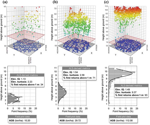
The selected model for estimating the AGB included the kurtosis, the interquartile range of the return heights and the percentage of first returns above 1 m high. Figure 3 presents these independent variables associated with the vertical distribution of ALS returns in three selected field plots representative of the P. halepensis forest under study. As can be observed, the AGB value of smaller pines in open areas (Figure 3(a)) is lower than in taller pines with little understory (Figure 3(c)). Thus, the AGB presents a direct relationship with these variables. The increases in the dispersion of the height values and in the percentage of first returns imply an increase in AGB content.

Figure 3. Metrics associated with the vertical distribution of ALS returns in three selected field plots representative of the P. halepensis forest: (a) smaller pines in open areas, (b) average height pines and (c) taller pines with little understory.

In Table 4, the squared partial correlation coefficient (Partial R²) describes how much of the dependent variable variance, which is not estimated by the other independent variables in the model, is estimated by each variable. The selected model, corresponding to step 3 in Table 4, shows that 55% of the variation in AGB has been explained by the addition here of the kurtosis as an explanatory variable. Similarly, 36% of the variation in AGB that is left unexplained by the interquartile range and the kurtosis is explained by the addition of the percentage of first returns above 1 m high. As a result, 84% of the variation in AGB is explained by these ALS-derived metrics related to the canopy height variability and canopy density. The selected model presents the smaller standard error of the estimate, being the most accurate prediction found.

Table 4. Summary of stepwise selection.

Step	Variables entered	Partial R^2	Model R^2	Standard error of the estimate	F-value	Probability level > F
1	% First returns above 1 m	0.57	0.59	18.53	56.56	0.00
2	% First returns above 1 m Elev. interquartile range	0.50 0.24	0.66	16.36	42.85	0.00
3	% First returns above 1 m Elev. interquartile range Elev. kurtosis	0.36 0.55 0.55	0.84	11.15	77.98	0.00

As shown in Table 5, the RMSE and the RMSEcv were 10.65 and 10.63 ton/ha, respectively. The percentage RMSE value is quite similar as those obtained by cross-validation (around 27%). The bias value of 0.03 ton/ha denotes a little overestimation of the model.

Table 5. Model summary of AGB estimation.

Predictive model	Fitting phase				Cross-validation
	R^2	RMSE	%RMSE	Bias	R^2	RMSEcv	%RMSEcv	Bias
AGB = −61114.30 + 20201.17∙Elev. interquartile range +10,184.62∙Elev. kurtosis + 520.98% first returns above 1 m	0.84	10.65	27.39	0.00	0.84	10.63	27.35	0.03

3.2. Error analysis

As can be seen in Table 6, all chi-square values obtained in the Kruskal–Wallis test using the residuals of the model were not significant, showing an asymptotic significance above 0.01. Thus, terrain slope, aspect, canopy cover, the number of laser returns and the scan angle do not influence AGB estimations at plot level.

Table 6. Kruskal–Wallis (K.W.) chi-square values for AGB.

Variable	K.W. chi-square	Asymptotic significance
Terrain slope	4.16	0.12
Aspect	1.40	0.50
Canopy cover	2.38	0.30
Quantity of laser returns	1.24	0.54
Scan angle	3.16	0.21

Statistical significance level at P-value <0.01.

3.3. Carbon dioxide emissions map

Figure 4 shows the AGB and the CO₂ emission after implementing the model and the conversion factors in a Geographic Information System (GIS) environment. The northwest part of the study area shows a heterogeneous P. halepensis forest with low stand density and high AGB values (above 50 ton/ha). These stands are older than the rest of the study area, this explains the high values of CO₂ emissions estimated (above 100.000 ton/ha) in case of wildfire. In contrast, the northeast part includes two distinct homogeneous areas in terms of AGB values. These areas differ in stand density and canopy height as in the past they were affected by several wildfires. In conclusion, there is a sharp contrast in the CO₂ values between regenerated and old pines, ranging from 20 to 100 ton/ha, respectively.

Figure 4. AGB (a) and CO₂ (b) emissions mapping of P. halepensis forest.

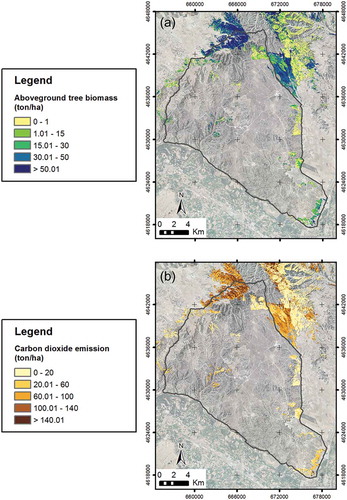
The 60% of the pine stands under study could emit up to 60 ton/ha of CO₂, although 20% of the study area could exceed 100 ton/ha of emissions. Thus, forest managers should focus fire protection measures in the last mentioned stands.

4. Discussion

Large amounts of the CO₂ are removed from the atmosphere and warehoused by forest ecosystems (Solomon et al. 2007), thus mitigating the magnitude of the global climate change. One of the most dynamic and largest carbon pools in forest ecosystems is the AGB stored by living trees (Ene et al. 2012).

In general, carbon inventory systems rely exclusively on ground network observations. In addition, regional arrays of ground plots and flux towers cannot always provide accurate local estimates or by land-use or cover classes (Gonzalez et al. 2010). As alternative, remote sensing systems has the potential to complement these terrestrial surveys for forest carbon estimation (Ene et al. 2012). The ALS remote sensing has been tested for biomass estimation in various forest types (Lefsky et al. 2002; Asner et al. 2008; Boudreau et al. 2008; Næsset ans Gobakken 2008; Næsset 2011; Ene et al. 2012) showing marked improvements in precision relative to conventional surveys for areas between 20 and 2000 km². Despite the wide acceptance of the use of ALS technology, little research has focused on P. halepensis, one of the most important species of the Mediterranean Basin using low-density point clouds. P. halepensis species usually shows irregular crown, disperse distribution and the leaf area of the forest is lower, compared to boreal forests in which there are lots of experiences using this technology (Maltamo, Næsset, and Vauhkonen 2014).

The results indicate that ALS-PNOA data, although captured at a low point density, can be used to estimate biomass in P. halepensis forest stands. The good fit of the linear model reveals suitability of the methodology. Although the RMSE around 11 ton/ha may seem high, it should be noted that the inventory data covered a wide range of values as can be observed in Table 1. This is frequently found in the literature, with individual plot-level estimates having a wide range of biomass (Zolkos, Goetz, and Dubayah 2013).

The ALS-derived metrics included in the model are significant and present a logical behavior with respect to the sign of the relationship. In this regard, it is common that prediction models include metrics directly related to the canopy height variability, as the dispersion and shape of the distribution of return heights, and to the canopy density (García, Godino, and Mauro 2012). Despite the low point density of the data used, high and significant correlations between AGB and metrics were found. It should be noted that the time delay between the ALS data acquisition and the field data collection was not considered a significant source of error, as it is documented that the pine forest under study did not change considerably during that period. Thinning operations and understory removal were only carried out at the roadsides in order to prevent and reduce the fire risk.

The R² value was similar to those obtained by other authors, such as Gonzalez-Ferreiro, Dieguez-Aranda, and Miranda (2012). In contrast to other studies, such as García et al. (2010), the logarithmic transformation of the original variables, commonly applied to achieve a better fit of the model or to meet the assumptions of the linear regression model, in this case produced worse results.

Bearing in mind that point density has a direct effect on ALS data acquisition costs (Maltamo, Næsset, and Vauhkonen 2014), our results using low-density ALS data support those presented by Gonzalez-Ferreiro, Dieguez-Aranda, and Miranda (2012). They pointed out that it is viable to estimate forest variables at stand level with low pulse densities (up to 0.5 points/m²). For example, Estornell et al. (2014) revealed the good performance for estimating volume (R² = 0.70) and total height (R² = 0.67) in olive tree plantations with a nominal pulse density of 0.5 points/m².

The Kruskal–Wallis analysis showed that the quantity of returns available per plot do not seem to be the cause of error in AGB estimates at plot level.

Thus, according to our results, the ALS-PNOA data becomes an excellent source of information for forest management, reducing forest inventory costs and improving CO₂ estimations. The aim of this research was to evaluate the emission previous to the possible case of fire. In this regard, it was decided to present the worst scenario of total combustion, especially considering that severity in this Mediterranean pine forest usually presents a dichotomous behavior (low or very high severity). Given that the ground cover by leaves is really complex to assess with remote sensing, this approach has been only focused in the tree fraction.

Extrapolation of the model to other areas seems to be a common problem with ALS data, since it is calibrated for relatively small area. However, transferability of equations or models is also a common problem to optical data as demonstrated by Foody, Boyd, and Cutler (2003). It should also be noted that the AGB model was based on allometric equations and therefore the accuracy of the model depends on the accuracy of the allometric equations employed. Nevertheless, this approach is commonly used due to the difficulty of developing specific equations that require destructive sampling for a large number of plots (García et al. 2010). Thus, this research provides the necessary motivation to perform future studies along different Mediterranean environments, in order to improve the detailed modeling of CO₂ emissions. It would be desirable to assess the suitability of the ALS-PNOA data to characterize other Mediterranean forest species in large areas in terms of carbon stock and emissions, in order to compare prediction accuracies and to increase the body of research in this topic.

Finally, in order to improve outcomes, different lines of research should be considered. First, nonparametric regression models based on machine learning techniques, such as random forest and support vector machines, should be explored in future as they have been used successfully in forest biomass components prediction (Maltamo, Næsset, and Vauhkonen 2014; Zhang et al. 2014). Second, as Isaev et al. (2002), Koch (2010), García et al. (2010) and Manzanera et al. (2016) suggested, the integration of ALS with other airborne and spaceborne sensors (multispectral or hyperspectral data and SAR) is a possible path of development to improve biomass models obtained. Furthermore, the ALS intensity-derived variables, which consider the variations in spectral response of canopy material in the near-infrared region, and the height metrics, could improve the accuracy according to García et al. (2010). However, a proper calibration of intensity data could not be accomplished.

Particularly, an additional effort should be directed to evaluate the biomass of understory because it can contribute to CO₂ emissions in a wildfire. Looking to the future, mapping of forest biomass and changes due to temporal variation (e.g. disturbance, anthropogenic management activities, and forest growth) will be possible if Spain finishes its second ALS coverage, already started in some regions in 2015. Having pre- and postfire ALS data could allow quantification of biomass loss due to consumption by the fire. Consequently, it will be possible estimating postfire CO₂ emissions from a burned area, improving the climate change mitigation efforts (Isaev et al. 2002).

Understanding the effect of hypothetical burning on AGB in terms of CO₂ releases could be of crucial importance for fuel management plans, especially in widespread flammable plantations, such as Mediterranean P. halepensis stands (Battipaglia et al. 2014).

5. Conclusions

The observations in the past last decades show that the increasing intensity and spread of forest fires in Mediterranean Basin are related to the rise in temperature and decline in precipitation in combination with the change in land use. Models of emission gases from AGB burning through forest fires are required to evaluate and represent the impact of biomass burning. The account of CO₂ emissions is essential for climate regulation policies and the evaluation of the effects of these policies, as well as for understanding the ecological services that forest provide to society.

This study demonstrates that the CO₂ emission of the AGB in case of a fire event can be modeled with reasonable precision in Mediterranean P. halepensis forest using low-density ALS data.

The regression model to estimate the AGB presented a R² value of 0.84, with %RMSE of 27.35%. The model included variables belonging to different types of ALS metrics: variables depicting vegetation height variability or return distribution, and measurements related to canopy density. Although regression equations for biomass estimation may be site specific, good relationships have been demonstrated. Then, CO₂ emissions in case of fire were mapped at a finer scale using conversion factors to transform the AGB into CO₂, which is useful in the context of forest managing.

It is important to notice that Mediterranean forests’ lack of the homogeneity of the boreal ones present a dense understory and a steeper relief, making more difficult the estimation of structural parameters with ALS data, even more with low point densities. That is the reason why in this study we move a step forward by analyzing the influence of such variables in AGB estimation. The results demonstrate that, for example, the number of returns per plot did not influence the AGB error, as well as the scan angle. This confirms the utility of the data for Mediterranean environment, not being necessary to eliminate the points with high scan angles.

Acknowledgments

This work has been financed by the Government of Aragón, Department of Science, Technology and University [FPI Grant BOA 30, 11/02/2011] and supported by the Research Project of Centro Universitario de la Defensa de Zaragoza [Project No: 2013-04]. The ALS data were provided by the Spatial Information Centre of Aragón. The authors are grateful to the Training Center (CENAD) “San Gregorio” for its assistance in the field and for its invaluable technical support and to the Army Geographic Center (CEGET) for providing the basic cartography.

Disclosure statement

No potential conflict of interest was reported by the authors.

Additional information

Funding

This work was supported by the Government of Aragón, Department of Science, Technology and University under Grant BOA 30, 11/02/2011; and Centro Universitario de la Defensa de Zaragoza under Research Project No: 2013-04;

References

- Andersen, H.-E., R. J. McGaughey, and S. E. Reutebuch. 2005. “Estimating Forest Canopy Fuel Parameters Using Lidar Data.” Remote Sensing of Environment 94 (4): 441–449. doi:10.1016/j.rse.2004.10.013.
- Asner, G. P., R. F. Hughes, T. A. Varga, D. E. Knapp, and T. Kennedy-Bowdoin. 2008. “Environmental and Biotic Controls over Aboveground Biomass Throughout a Tropical Rain Forest.” Ecosystems 12 (2): 261–278. doi:10.1007/s10021-008-9221-5.
- Battipaglia, G., S. Strumia, A. Esposito, E. Giuditta, C. Sirignano, S. Altieri, and F. A. Rutigliano. 2014. “The Effects of Prescribed Burning on Pinus halepensis Mill. as Revealed by Dendrochronological and Isotopic Analyses.” Forest Ecology and Management 334 (December): 201–208. doi:10.1016/j.foreco.2014.09.010.
- Bortolot, Z. J., and R. H. Wynne. 2005. “Estimating Forest Biomass Using Small Footprint Lidar Data: An Individual Tree-Based Approach that Incorporates Training Data.” ISPRS Journal of Photogrammetry and Remote Sensing 59 (6): 342–360. doi:10.1016/j.isprsjprs.2005.07.001.
- Boudreau, J., R. F. Nelson, H. A. Margolis, A. Beaudoin, L. Guindon, and D. S. Kimes. 2008. “Regional Aboveground Forest Biomass Using Airborne and Spaceborne Lidar in Québec.” Remote Sensing of Environment 112 (10): 3876–3890. doi:10.1016/j.rse.2008.06.003.
- Bouvier, M., S. Durrieu, R. A. Fournier, and J.-P. Renaud. 2015. “Generalizing Predictive Models of Forest Inventory Attributes Using an Area-Based Approach with Airborne Lidar Data.” Remote Sensing of Environment 156 (0): 322–334. doi:10.1016/j.rse.2014.10.004.
- Bujarrabal, E. 2009. “El Pino Carrasco (Pinus halepensis Miller) En Aragón. Una Conífera Valiosa Por Su Función Protectora.” Naturaleza Aragonesa: Revista De La Sociedad De Amigos Del Museo Paleontológico De La Universidad De Zaragoza 23: 45–55.
- Carvalho, J. A., S. S. Amaral, M. A. M. Costa, T. G. Soares Neto, C. A. G. Veras, F. S. Costa, T. T. Van Leeuwen, et al. 2016. “CO2 and CO Emission Rates from Three Forest Fire Controlled Experiments in Western Amazonia.” Atmospheric Environment 135 :73–83. doi:10.1016/j.atmosenv.2016.03.043.
- Chen, Q., P. Gong, D. Baldocchi, and Y. Q. Tian. 2007. “Estimating Basal Area and Stem Volume for Individual Trees from Lidar Data.” Photogrammetric Engineering & Remote Sensing 73 (12): 1355–1365. doi:10.14358/PERS.73.12.1355.
- Chuvieco, E. 2009. Earth Observation of Wildland Fires in Mediterranean Ecosystems. Alcalá de Henares: Springer.
- Clark, M. L., D. B. Clark, and D. A. Roberts. 2004. “Small-Footprint Lidar Estimation of Sub-Canopy Elevation and Tree Height in a Tropical Rain Forest Landscape.” Remote Sensing of Environment 91 (1): 68–89. doi:10.1016/j.rse.2004.02.008.
- Cohen, W. B., and T. A. Spies. 1992. “Estimating Structural Attributes of Douglas-Fir/Western Hemlock Forest Stands from Landsat and SPOT Imagery.” Remote Sensing of Environment 41 (1): 1–17. doi:10.1016/0034-4257(92)90056-P.
- Ene, L. T., E. Næsset, T. Gobakken, T. G. Gregoire, G. Ståhl, and R. Nelson. 2012. “Assessing the Accuracy of Regional Lidar-Based Biomass Estimation Using a Simulation Approach.” Remote Sensing of Environment 123 (August): 579–592. doi:10.1016/j.rse.2012.04.017.
- Estornell, J., B. Velázquez-Martí, I. López-Cortés, D. Salazar, and A. Fernández-Sarría. 2014. “Estimation of Wood Volume and Height of Olive Tree Plantations Using Airborne Discrete-Return Lidar Data.” GIScience & Remote Sensing 51 (1): 17–29. doi:10.1080/15481603.2014.883209.
- Evans, J., A. Hudak, R. Faux, and A. M. Smith. 2009. “Discrete Return Lidar in Natural Resources: Recommendations for Project Planning, Data Processing, and Deliverables.” Remote Sensing 1 (4): 776–794. doi:10.3390/rs1040776.
- Evans, J. S., and A. T. Hudak. 2007. “A Multiscale Curvature Algorithm for Classifying Discrete Return Lidar in Forested Environments.” IEEE Transactions on Geoscience and Remote Sensing 45 (4): 1029–1038. doi:10.1109/TGRS.2006.890412.
- Foody, G. M., D. S. Boyd, and M. E. J. Cutler. 2003. “Predictive Relations of Tropical Forest Biomass from Landsat TM Data and Their Transferability between Regions.” Remote Sensing of Environment 85 (4): 463–474. doi:10.1016/S0034-4257(03)00039-7.
- Fournier, T. P., G. Battipaglia, B. Brossier, and C. Carcaillet. 2013. “Fire-Scars and Polymodal Age-Structure Provide Evidence of Fire-Events in an Aleppo Pine Population in Southern France.” Dendrochronologia 31 (3): 159–164. doi:10.1016/j.dendro.2013.05.001.
- García, D., M. Godino, and F. Mauro. 2012. Lidar: Aplicación Práctica Al Inventario Forestal. Lexington, USA: Editorial Academia Española. http://books.google.es/books?id=YIatMAEACAAJ.
- García, M., R. David, E. Chuvieco, and F. M. Danson. 2010. “Estimating Biomass Carbon Stocks for a Mediterranean Forest in Central Spain Using Lidar Height and Intensity Data.” Remote Sensing of Environment 114 (4): 816–830. doi:10.1016/j.rse.2009.11.021.
- García-Martín, A., F. Pérez-Cabello, J. de la Riva Fernández, and R. Montorio Llovería. 2008. 'Estimation Of Crown Biomass Of Pinus Spp. From Landsat Tm And Its Effect On Burn Severity In A Spanish Fire Scar'. IEEE Journal of Selected Topics in Applied Earth Observations and Remote Sensing 1 (4): 254-265. doi:10.1109/JSTARS.2008.2011623
- García-Martín, A., J. de la Riva, F. Pérez-Cabello, and R. Montorio. 2012. 'Using Remote Sensing To Estimate A Renewable Resource: Forest Residual Biomass'. In Remote Sensing of Biomass: Principles and Applications, edited by Temilola Fatoyinbo, 297-322. Rijeka, Croatia: InTech. (ISBN: 978-953-51-0313-4).
- Gatziolis, D., and H.-E. Andersen. 2008. A Guide to LIDAR Data Acquisition and Processing for the Forests of the Pacific Northwest. http://www.treesearch.fs.fed.us/pubs/30652.
- Gazol, A., M. Ribas, E. Gutiérrez, and J. J. Camarero. 2017. “Aleppo Pine Forests from across Spain Show Drought-Induced Growth Decline and Partial Recovery.” Agricultural and Forest Meteorology 232 (January): 186–194. doi:10.1016/j.agrformet.2016.08.014.
- Gonzalez, P., G. P. Asner, J. J. Battles, M. A. Lefsky, K. M. Waring, and M. Palace. 2010. “Forest Carbon Densities and Uncertainties from Lidar, Quickbird, and Field Measurements in California.” Remote Sensing of Environment 114 (7): 1561–1575. doi:10.1016/j.rse.2010.02.011.
- Gonzalez-Ferreiro, E., U. Dieguez-Aranda, and D. Miranda. 2012. “Estimation of Stand Variables in Pinus radiata D. Don Plantations Using Different Lidar Pulse Densities.” Forestry 85 (2): 281–292. doi:10.1093/forestry/cps002.
- González-Olabarria, J.-R., F. Rodríguez, A. Fernández-Landa, and B. Mola-Yudego. 2012. “Mapping Fire Risk in the Model Forest of Urbión (Spain) Based on Airborne Lidar Measurements.” Forest Ecology and Management 282 (0): 149–156. doi:10.1016/j.foreco.2012.06.056.
- Goodwin, N. R., N. C. Coops, and D. S. Culvenor. 2006. “Assessment of Forest Structure with Airborne Lidar and the Effects of Platform Altitude.” Remote Sensing of Environment 103 (2): 140–152. doi:10.1016/j.rse.2006.03.003.
- Hair, J. F., R. E. Anderson, R. L. Tatham, and W. C. Black. 1999. Análisis Multivariante, 5a. Madrid: Prentice Hall Iberia.
- Holmgren, J., M. Nilsson, and H. Olsson. 2003. “Simulating the Effects of Lidar Scanning Angle for Estimation of Mean Tree Height and Canopy Closure.” Canadian Journal of Remote Sensing 29 (5): 623–632. doi:10.5589/m03-030.
- Isaev, A. S., G. N. Korovin, S. A. Bartalev, D. V. Ershov, A. Janetos, E. S. Kasischke, H. H. Shugart, N. H. F. French, B. E. Orlick, and T. L. Murphy. 2002. “Using Remote Sensing to Assess Russian Forest Fire Carbon Emissions.” Climatic Change 55 (1): 235–249. doi:10.1023/A:1020221123884.
- Jakubowski, M. K., Q. Guo, and M. Kelly. 2013. “Tradeoffs between Lidar Pulse Density and Forest Measurement Accuracy.” Remote Sensing of Environment 130 (March): 245–253. doi:10.1016/j.rse.2012.11.024.
- Koch, B. 2010. “Status and Future of Laser Scanning, Synthetic Aperture Radar and Hyperspectral Remote Sensing Data for Forest Biomass Assessment.” ISPRS Journal of Photogrammetry and Remote Sensing 65 (6): 581–590. doi:10.1016/j.isprsjprs.2010.09.001.
- Kraus, K., and N. Pfeifer. 1998. “Determination of Terrain Models in Wooded Areas with Airborne Laser Scanner Data.” ISPRS Journal of Photogrammetry and Remote Sensing 53 (4): 193–203. doi:10.1016/s0924-2716(98)00009-4.
- Leboeuf, A., A. Beaudoin, R. A. Fournier, L. Guindon, J. E. Luther, and M. C. Lambert. 2007. “A Shadow Fraction Method for Mapping Biomass of Northern Boreal Black Spruce Forests Using Quickbird Imagery.” Remote Sensing of Environment 110 (4): 488–500. doi:10.1016/j.rse.2006.05.025.
- Lee, S. J., J. R. Kim, and Y. S. Choi. 2013. “The Extraction of Forest CO2 Storage Capacity Using High-Resolution Airborne Lidar Data.” GIScience & Remote Sensing 50 (2): 154–171. doi:10.1080/15481603.2013.786957.
- Lefsky, M.A., W.B. Cohen, D.J. Harding, G.G. Parker, S.A. Acker, and S.T. Gower. 2002. “Lidar Remote Sensing Of Above-ground Biomass In Three Biomes.” Global ecology And Biogeography 11 (5): 393–399. doi: 10.1016/S0034-4257(99)00057-7.
- Lim, K. S., and P. M. Treitz. 2004. “Estimation of above Ground Forest Biomass from Airborne Discrete Return Laser Scanner Data Using Canopy-Based Quantile Estimators.” Scandinavian Journal of Forest Research 19 (6): 558–570. doi:10.1080/02827580410019490.
- Liu, S., X. Su, S. Dong, F. Cheng, H. Zhao, X. Wu, X. Zhang, and J. Li. 2015. “Modeling Aboveground Biomass of an Alpine Desert Grassland with SPOT-VGT NDVI.” GIScience & Remote Sensing 52 (6): 680–699. doi:10.1080/15481603.2015.1080143.
- Lu, D. 2006. The Potential and Challenge of Remote sensing‐based Biomass Estimation. International Journal of Remote Sensing 27 (7): 1297–1328. doi:10.1016/S0034-4257(03)00139-1.
- Maltamo, M., E. Næsset, and J. Vauhkonen. 2014. Forestry Applications of Airborne Laser Scanning: Concepts and Case Studies. Managing Forest Ecosystems. London: Springer.
- Manzanera, J. A., A. García-Abril, C. Pascual, R. Tejera, S. Martín-Fernández, T. Tokola, and R. Valbuena. 2016. “Fusion of Airborne Lidar and Multispectral Sensors Reveals Synergic Capabilities in Forest Structure Characterization.” GIScience & Remote Sensing 53 (6): 723–738. doi:10.1080/15481603.2016.1231605.
- McGaughey, R. 2009. FUSION/LDV: Software for LIDAR Data Analysis and Visualization. Seattle, WA: US Department of Agriculture, Forest Service, Pacific Northwest Research Station.
- Means, J. E., S. A. Acker, B. J. Fitt, M. Renslow, L. Emerson, and C. J. Hendrix. 2000. “Predicting Forest Stand Characteristics with Airborne Scanning Lidar.” Photogrammetric Engineering and Remote Sensing 66 (11): 1367–1371.
- Meng, Q., C. J. Cieszewski, M. Madden, and B. Borders. 2007. “A Linear Mixed-Effects Model of Biomass and Volume of Trees Using Landsat ETM+ Images.” Forest Ecology and Management 244 (1–3): 93–101. doi:10.1016/j.foreco.2007.03.056.
- Mieville, A., C. Granier, C. Liousse, B. Guillaume, F. Mouillot, J. F. Lamarque, J. M. Grégoire, and G. Pétron. 2010. “Emissions of Gases and Particles from Biomass Burning during the 20th Century Using Satellite Data and an Historical Reconstruction.” Atmospheric Environment 44 (11): 1469–1477. doi:10.1016/j.atmosenv.2010.01.011.
- Montealegre, A., M. T. Lamelas, and J. De La Riva. 2015. “Interpolation Routines Assessment in ALS-Derived Digital Elevation Models for Forestry Applications.” Remote Sensing 7 (7): 8631. doi:10.3390/rs70708631.
- Montero, G., R. Ruiz-Peinado, and M. Muñoz. 2005. “Producción De Biomasa Y Fijación De CO2 Por Los Bosques Españoles.” Edited by. In Instituto Nacional De Investigación Y Tecnología Agraria Y Alimentaria Ministerio De Educación Y Ciencia. Torrejón de Ardoz: Monografías INIA: Serie Forestal 13.
- Moriondo, M., P. Good, R. Durao, M. Bindi, C. Giannakopoulos, and J. CorteReal. 2006. “Potential Impact of Climate Change on Fire Risk in the Mediterranean Area.” Climate Research 31 (1): 85–95. doi:10.3354/cr031085.
- Moya, D., J. De Las Heras, F. R. López-Serrano, and V. Leone. 2008. “Optimal Intensity and Age of Management in Young Aleppo Pine Stands for Post-Fire Resilience.” Forest Ecology and Management 255 (8–9): 3270–3280. doi:10.1016/j.foreco.2008.01.067.
- Muukkonen, P., and J. Heiskanen. 2007. “Biomass Estimation over A Large Area Based on Standwise Forest Inventory Data and ASTER and MODIS Satellite Data: A Possibility to Verify Carbon Inventories.” Remote Sensing of Environment 107 (4): 617–624. doi:10.1016/j.rse.2006.10.011.
- Naesset, E. 2002. “Predicting Forest Stand Characteristics with Airborne Scanning Laser Using a Practical Two-Stage Procedure and Field Data.” Remote Sensing of Environment 80 (1): 88–99. doi:10.1016/S0034-4257(01)00290-5.
- Næsset, E. 2011. “Estimating Above-Ground Biomass in Young Forests with Airborne Laser Scanning.” International Journal of Remote Sensing 32 (2): 473–501. doi:10.1080/01431160903474970.
- Næsset, E., and T. Gobakken. 2008. “'Estimation Of Above- And Below-ground Biomass Across Regions Of The Boreal Forest Zone Using Airborne Laser'.” Remote Sensing Of Environment 112 (6): 3079–3090. doi: 10.1016/j.rse.2008.03.004.
- Naesset, E., and T. Okland. 2002. “Estimating Tree Height and Tree Crown Properties Using Airborne Scanning Laser in a Boreal Nature Reserve.” Remote Sensing of Environment 79 (1): 105–115. doi:10.1016/S0034-4257(01)00243-7.
- Nilsson, M. 1996. “Estimation of Tree Heights and Stand Volume Using an Airborne Lidar System.” Remote Sensing of Environment 56 (1): 1–7. doi:10.1016/0034-4257(95)00224-3.
- Pan, Y., R. A. Birdsey, J. Fang, R. Houghton, P. E. Kauppi, W. A. Kurz, O. L. Phillips, et al. 2011. “A Large and Persistent Carbon Sink in the World’s Forests.” Science 333 (6045): 988. doi:10.1126/science.1201609.
- Patenaude, G., R. A. Hill, R. Milne, D. L. A. Gaveau, B. B. J. Briggs, and T. P. Dawson. 2004. “Quantifying Forest above Ground Carbon Content Using Lidar Remote Sensing.” Remote Sensing of Environment 93 (3): 368–380. doi:10.1016/j.rse.2004.07.016.
- Pausas, J. G., J. Llovet, A. Rodrigo, and R. Vallejo. 2008. “Are Wildfires a Disaster in the Mediterranean Basin? – A Review.” International Journal of Wildland Fire 17 (6): 713–723. doi:10.1071/WF07151.
- Popescu, S. C. 2007. “Estimating Biomass of Individual Pine Trees Using Airborne Lidar.” Biomass and Bioenergy 31 (9): 646–655. doi:10.1016/j.biombioe.2007.06.022.
- Renslow, M. 2013. “Manual of Airborne Topographic Lidar.” Bethesda: The American Society for Photogrammetry and Remote Sensing.
- Rosette, J., J. Suárez, R. Nelson, S. Los, B. Cook, and P. North. 2012. “Lidar Remote Sensing for Biomass Assessment.” In Remote Sensing of Biomass: Principles and Applications, edited by T. Fatoyinbo, 3–26. Rijeka, Croatia: InTech.
- Ruiz-Peinado, R., M. Del Rio, and G. Montero. 2011. “New Models for Estimating the Carbon Sink Capacity of Spanish Softwood Species.” Forest Systems 20 (1): 176–188. doi:10.5424/fs/2011201-11643.
- Sačkov, I., G. Santopuoli, T. Bucha, B. Lasserre, and M. Marchetti. 2016. “Forest Inventory Attribute Prediction Using Lightweight Aerial Scanner Data in a Selected Type of Multilayered Deciduous Forest.” Forests 7 (12): 307. doi:10.3390/f7120307.
- Saranya, K. R. L., C. Sudhakar Reddy, and P. V. V. Prasada Rao. 2016. “Estimating Carbon Emissions from Forest Fires over a Decade in Similipal Biosphere Reserve, India.” Remote Sensing Applications: Society and Environment 4 (October): 61–67. doi:10.1016/j.rsase.2016.06.001.
- Solomon, S., D. Qin, M. Manning, Z. Chen, M. Marquis, K. Averyt, M. Tignor, and H. L. Miller. 2007.‘IPCC, 2007: Climate Change 2007: The Physical Science Basis. Contribution of Working Group I to the Fourth Assessment Report of the Intergovernmental Panel on Climate Change’. Cambridge, United Kingdom and New York.
- Tanase, M., J. De La Riva, and F. Pérez-Cabello. 2011. “Estimating Burn Severity at the Regional Level Using Optically Based Indices.” Canadian Journal of Forest Research 41 (4): 863–872. doi:10.1139/x11-011.
- Tanase, M. A., R. Panciera, K. Lowell, S. Tian, A. García-Martín, and J. P. Walker. 2014. “Sensitivity of L-Band Radar Backscatter to Forest Biomass in Semiarid Environments: A Comparative Analysis of Parametric and Nonparametric Models.” IEEE Transactions on Geoscience and Remote Sensing 52 (8): 4671–4685. doi:10.1109/TGRS.2013.2283521.
- Thomas, R. Q., G. C. Hurtt, R. Dubayah, and M. H. Schilz. 2008. “Using Lidar Data and a Height-Structured Ecosystem Model to Estimate Forest Carbon Stocks and Fluxes over Mountainous Terrain.” Canadian Journal of Remote Sensing 34 (sup2): S351–63. doi:10.5589/m08-036.
- Treitz, P., K. Lim, M. Woods, D. Pitt, D. Nesbitt, and D. Etheridge. 2012. “Lidar Sampling Density for Forest Resource Inventories in Ontario, Canada.” Remote Sensing 4 (4): 830–848. doi:10.3390/rs4040830.
- Trozzi, C., R. Vaccaro, and E. Piscitello. 2002. “Emissions Estimate from Forest Fires: Methodology, Software and European Case Studies.” In Emission Inventories - Partnering for the Future. Atlanta, USA: U.S. Environmental Protection Agency. Office of Air Quality Planning and Standards, Emission Factor and Inventory Group.
- Vauhkonen, J., L. Ene, S. Gupta, J. Heinzel, J. Holmgren, J. Pitkanen, S. Solberg, et al. 2012. “Comparative Testing of Single-Tree Detection Algorithms under Different Types of Forest.” Forestry 85 (1): 27–40. DOI:10.1093/forestry/cpr051.
- Vicente-Serrano, S. M., T. Lasanta, and C. Gracia. 2010. “Aridification Determines Changes in Forest Growth in Pinus halepensis Forests under Semiarid Mediterranean Climate Conditions.” Agricultural and Forest Meteorology 150 (4): 614–628. doi:10.1016/j.agrformet.2010.02.002.
- Vosselman, G., and H.-G. Maas. 2010. Airborne and Terrestrial Laser Scanning. Dunbeath: Whittles Publishing.
- Watt, M., A. Meredith, P. Watt, and A. Gunn. 2013. “Use of Lidar to Estimate Stand Characteristics for Thinning Operations in Young Douglas-Fir Plantations.” New Zealand Journal of Forestry Science 43 (18): 1–10. doi:10.1186/1179-5395-43-1.
- Zhang, J., S. Huang, E. H. Hogg, V. Lieffers, Y. Qin, and F. He. 2014. “Estimating Spatial Variation in Alberta Forest Biomass from a Combination of Forest Inventory and Remote Sensing Data.” Biogeosciences 11 (10): 2793–2808. doi:10.5194/bg-11-2793-2014.
- Zolkos, S. G., S. J. Goetz, and R. Dubayah. 2013. “A Meta-Analysis of Terrestrial Aboveground Biomass Estimation Using Lidar Remote Sensing.” Remote Sensing of Environment 128 (0): 289–298. doi:10.1016/j.rse.2012.10.017.