Developing soil indices based on brightness, darkness, and greenness to improve land surface mapping accuracy

Abstract

Soil, as one of the three basic biophysical components, has been understudied using remote sensing techniques compared to vegetation and impervious surface areas (ISA). This study characterized land surfaces based on the brightness–darkness–greenness model. These three dimensions, brightness, darkness, and greenness, were represented by the first Tasseled Cap Transformation (TC1), Normalize Difference Snow Index (NDSI), and Normalized Difference Vegetation Index (NDVI), respectively. The Ratio Index for Bright Soil (RIBS) was developed based on TC1 and NDSI, and the Product Index for Dark Soil (PIDS) was established by TC1 and NDVI. Their applications to the Landsat 8 Operational Land Imager images and 500 m 8-day composite Moderate Resolution Imaging Spectroradiometer (MODIS) in China revealed the efficiency. The two soil indices proficiently highlighted soil covers with consistently the smallest values, due to larger TC1 and smaller NDSI values in bright soil, and smaller NDVI and TC1 values in dark soil. The RIBS is capable of distinguishing bright soil from ISA without masking vegetation and water body. The spectral separability bright soil and ISA were perfect, with a Jeffries–Matusita distance of 1.916. And the PIDS was the only soil index that could discriminate dark soil from other land covers including ISA. The soil areas in China were classified using a simple threshold method based on MODIS images. An overall accuracy of 94.00% was obtained, with the kappa index of 0.8789. This study provided valuable insights into developing indices for characterizing land surfaces from different perspectives.

Keywords:

• Soil index
• brightness–darkness–greenness (B–D–G) model
• Vegetation–impervious–soil model
• Tasseled Cap Transformation
• Separability

1. Introduction

Over the past decades, land use/cover changes have taken place at an unprecedented rate around the world (Ellis and Pontius 2007), particularly in many countries such as China (Liu et al. 2003). Land use/cover changes such as urbanization, deforestation, and desertification can result in numerous environmental consequences to human society (Yang et al. 2005; Xu 2010; Müller, Griffiths, and Hostert 2016). Remote sensing images provide an efficient measure for monitoring and assessing land use/cover spatial–temporal changes (Guo and Du 2017). Multiple spectral variables are needed for accurate characterization of land cover types and detection of transitions from remote sensing images (Zhu and Woodcock 2014; Gómez, White, and Wulder 2016).

According to the vegetation–impervious–soil model proposed by Ridd (1995), all land cover types (other than water) can be regarded as a combination of three basic biophysical components: vegetation, impervious surface areas (ISA), and soil. Multiple spectral indices have been developed for the former two basic biophysical components in order to characterize and highlight them. For example, commonly applied vegetation indices include the Normalized Difference Vegetation Index (NDVI) (Becker and Choudhury 1988), the Enhanced Vegetation Index (EVI) (Huete et al. 2002), and the 2-band Enhanced Vegetation Index (EVI2) (Jiang et al. 2008). Spectral indices for impervious surfaces comprise the Normalized Difference Built-up Index (NDBI) (Zha, Gao, and Ni 2003), the Normalized Difference Impervious Surface Index (Xu 2010), the Biophysical Composition Index (BCI) (Deng and Wu 2012), and the Enhanced Built-up and Bareness Index (As-Syakur, Adnyana, and Nuarsa 2012).

Although it is recognized that multiple spectral variables are required for generation of rich and detailed land cover dynamics databases over large areas (Gómez, White, and Wulder 2016), few spectral indices have been proposed for the third basic biophysical component: soil (Deng et al. 2015). The development of soil indices for remote sensing image classification is challenging due to the following two reasons. One reason is the confusion between soil and impervious surfaces (Deng et al. 2015). It has been proved to be difficult to discriminate soil from ISA (Roberts et al. 2012). The other reason is the complexity of soil spectral signatures. The soil’s spectral signatures varied with its construction, texture, color, and surface roughness, and thus different soil types demonstrated significant different spectral characteristics (Lõhmus, Oja, and Lasn 1989; Deng and Wu 2012).

Developing soil indices that could efficiently distinguish soil cover from others would benefit the land use/cover change research community. Developing indices for one of the three basic biophysical components will greatly enrich existing spectral indices. It can easily accomplish one of the great missions for impervious spectral indices: separating soil from impervious surfaces (Xu 2010; As-Syakur, Adnyana, and Nuarsa 2012; Deng and Wu 2012; Zha, Gao, and Ni 2003). Therefore, the land surfaces covered by the basic biophysical components except vegetation could be better characterized through combined utilizations of both soil and impervious spectral indices.

To the best of our knowledge, the only existed soil index is the recently proposed Ratio Normalized Difference Soil Index (RNDSI) (Deng et al. 2015). The RNDSI was designed for extracting soil in urban/suburban environments using Landsat images in two counties in the United States (Deng et al. 2015). Its applicability to both urban and nonurban environments in other regions has not been examined yet, and the ability of RNDSI to separate sandy soil from ISA is questionable (Deng et al. 2015). Soil is a complex combination with various chemical and physical components, and the complex interactions between components in soils may make the theoretical models impractical (Ben-Dor 2002). Thus, empirical indices needed to be incorporated to discriminate soils from other land use/cover. This paper aims to develop soil indices through an empirical approach in order to distinguish soil from impervious surfaces and vegetation areas. The land cover of soil, which also referred as bare land, often included bright soil (sand desert and bright-colored soil) and dark soil (Gobi Desert and dark-colored soil). Given the complexity of the soil, two indices were proposed for bright soil and dark soil, individually. The developed soil indices were designed to be capable of highlighting soil cover from multiple categories of images over large regions.

The remainder of this paper is organized as follows. The next section presents the study area and data sources. Section 3 describes the development process for soil indices. The results of applying the proposed soil indices with Landsat images and a comparative analysis with the RNDSI are provided in Section 4.1, followed by further applications on MODIS images in Section 4.2 and discussion in Section 5.

2. Study area and data source

2.1. Study area

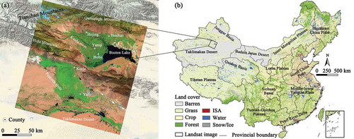
For developing soil indices, one scene Landsat image in the Mongolian Autonomous Prefecture of Bayingolin, China was applied. It covered six counties, including Korla, Bohu, Heshuo, Hejing, Yuli, and Yanqi Hui Autonomous Counties (Figure 1(a)). There were diverse land covers in this study area. For soil cover, there were two groups: the bright soil and dark soil. The bright soil, primary the sand desert, is distributed in the south at the edge of the Taklimakan Desert. The dark soil, primarily the Gobi Desert, is located at the foot of Hola Mountain in the west portion. Due to the Bosten Lake, the largest inland freshwater lake in China, there were large sown areas (5445.71 km²), primarily cultivated by cotton, spring wheat, and cole (http://tjj.xjbz.gov.cn/tjnj/xjbztjjnj2015/indexch.htm). For applications of these two indices, both Landsat images and Moderate Resolution Imaging Spectroradiometer (MODIS) for the whole county, China, were selected. The main land covers included forest, crop, grass, barren, water body, and ISA, with reference to the 1-km land use/cover distribution map in 2000 (Figure 1(b)) provided by Environmental and Ecological Science Data Center for West China at the National Natural Science Foundation of China (http://westdc.westgis.ac.cn) (Ren et al. 2012). The barren was principally distributed in the Northwest China (Figure 1(b)) (Yang et al. 2005).

Figure 1. The spatial distribution maps of (a) Landsat image (band combination 7, 5, 3) and (b) land cover of China.

2.2. Data sources

2.2.1. Remote sensing images

Two categories of remote sensing imagery with different spatial and spectral resolutions were utilized: Landsat 8 Operational Land Imager (OLI) images and MODIS images. Landsat 8 images are superior to Landsat 7 ETM+ images because they get rid of gap problems and provide quality assessment bands. A scene of a cloud-free Landsat 8 image (143/031) acquired on 19 September 2015 in the Mongolian Autonomous Prefecture of Bayingolin, China was exploited. The MODIS Terra MOD09A1 Version 6 product in China in 2015 were used. For each pixel, any 8-day composite identified with cloud contaminations from the quality control flag layer was excluded. The images were geometrically corrected with pixel values representing surface reflectance. Atmospheric correction was not carried out for Landsat images due to cloud-free atmospheric conditions. The Universal Transverse Mercator projection and WGS 84 datum were applied to both MODIS and Landsat images.

2.2.2. Reference datasets

Reference datasets were collected from field surveys and also acquired directly from Google Earth images through visual interpretation (Sheppard and Cizek 2009). For the assessments of soil indices from Landsat 8 OLI images, a total of 1523 reference sites were gathered, including 408 sites of croplands, 60 sites of meadows, 458 sites of bright soil, 235 sites of water bodies, 98 sites of ISA, and 264 sites of dark soil. To evaluate the soil indices from MODIS images in China, field surveys were carried out in early August 2012; early February, late April, and late July 2013; mid-January and August 2014; mid-February, early August and December 2015; and early February, late March and April 2016, respectively. UniStrong G138 or MG858 hand-held GPS receivers were utilized for ground surveys at field sites. At each sampling site, the land cover and vegetation cover density were recorded. A total of 2808 reference sites were collected. Of these sites, 349, 767, 164, 140, and 507 sites were cropland, woodland, meadow, water body, and ISA, respectively. The remaining sites were bare soil: 786 sites of bright soil and 95 sites of dark soil.

3. Methodology

3.1. Reinvestigating the brightness–darkness–greenness model in characterizing land surfaces

The brightness–darkness–greenness (B–D–G) model is a scene model that can be applied in a wide variety of urban landscape evolution studies (Yue et al. 2014; Strahler, Woodcock, and Smith 1986; Kauth and Thomas 1976). This study demonstrated that the land surfaces including urban, soil, and vegetation landscapes can be characterized by the B–D–G model. The greenness could be described by vegetation indices such as the Normalized Difference Vegetation Index (NDVI) (Huete et al. 2002), representing vegetation cover density. The dimension of greenness is the most often studied for various purposes especially for highlighting vegetation (Qiu, Liu et al. 2016). The dimension of brightness can be derived from the first Tasseled Cap Transformation (TC1) (Baig et al. 2014; Zhang et al. 2002), which have been successfully utilized to developing spectral indices for ISA and soil (Deng and Wu 2012; Deng et al. 2015). Compared with greenness and brightness, less attention was paid to the dimension of darkness. The land surface darkness was computed by the Normalize Difference Snow Index (NDSI). The NDSI combining band 3 and 6 (green and shortwave infrared red band 1) was applied (Salomonson and Appel 2004).

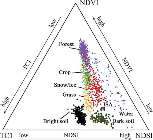
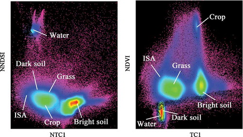
The triangular scatterplot of these three spectral indices, TC1, NDSI, and NDVI, was shown in Figure 2 in order to illustrate the processes. Different land covers were distinguished from each other, particularly the bright soil and dark soil. The bright soil was characterized as higher values of brightness (TC1), smaller values of darkness (NDSI_(3–6)) and greenness (NDVI). The dark soil was illustrated with smaller values of darkness and greenness. Therefore, this approach can develop soil indices for the bright and dark soil based on these three dimensions: brightness, darkness, and greenness.

Figure 2. Triangular scatterplot of NDVI, TC1, and NDSI.

3.2. Developing soil indices

A reexamination of relationships between NDSI, TC1, and NDVI was conducted to further design the soil indices in details. The NDSI and TC1 were normalized to range 0–1 before analyzing their associations. As shown in the scatterplot of the normalized NDSI and TC1 (Figure 3(a)), bright soil was distinguished with larger TC1 and lower NDSI values. In contrast, the water body exhibited with lower TC1 and higher NDSI values. Consequently, the bright soil and water body were scattered in the bottom right and top left corner in the scatterplot, respectively (Figure 3(a)). The ISA, crop, grass, and dark soil were scattered between the water body and the bright soil. Therefore, a Ratio Index for Bright Soil (RIBS) was designed based on NDSI and TC1. Through dividing NDSI by TC1, bright soil was expected to obtain the lowest values.

Figure 3. The scatterplot between (a) NDSI and TC1, (b) TC1 and NDVI from different land covers.

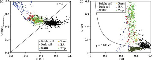
In the scatterplot of NDVI and TC1, the dark soil, bright soil, and crop formed a triangle (Figure 3(b)). Compared with other land covers, the dark soil was characterized with low values in both NDVI and TC1. Consequently, another Product Index for Dark Soil (PIDS) was developed based on NDVI and TC1. Formulas for RIBS and PIDS are provided in functions (1) and (2).

(1) $RIBS=\frac{NNDS{I}_{(3-6)}}{NTC1},$(1)

$\mathrm{w}\mathrm{h}\mathrm{e}\mathrm{r}\mathrm{e}NNDS{I}_{(3-6)}={\frac{NDS{I}_{(3-6)}-NDS{I}_{(3-6)min}}{NDS{I_{(3-6)}}_{max}-NDS{I_{(3-6)}}_{min}}}_{ },NDS{I}_{(3-6)}=\frac{Green-SWIR{ }_1^{ }}{Green+SWI{R}_1},\mathrm{a}\mathrm{n}\mathrm{d}NTC1=\frac{TC1-TC{1}_{min}}{TC{1}_{max}-TC{1}_{min}}$

(2) $PIDS=TC1\ast NDVI,$(2)

where TC1_max and TC1_min are the maximum and minimum values, respectively, of the TC1 component; and NDSI_(3–6)max and NDSI_(3–6)min are the maximum and minimum values, respectively, of the NDSI_(3–6). The numerical subscript of spectral indices in this study indicated the corresponding spectral bands from Landsat 8 image.

3.3. Performance assessment

The performance of the RIBS and PIDS was evaluated through two aspects: spectral separability and classification accuracy. Spectral separability was measured by the Spectral Discrimination Index (SDI) and the Jeffries–Matusita (JM) distance (Van Niel, McVicar, and Datt 2005; Wardlow, Egbert, and Kastens 2007). The SDI was designed to measure the degree of spectral separation between two land cover types (Radeloff, Mladenoff, and Boyce 1999). In addition to the SDI, the JM distance also provided a general measure of separability between two classes according to their probability (Wardlow, Egbert, and Kastens 2007). Greater SDI values and JM distances indicated better separability. Specifically, a SDI of greater than 1 revealed reasonable separability. The JM distance ranges between 0 and 2. Values of the JM distance of lower than 1 suggested the two classes were poorly separable (Deng and Wu 2012) and values close to 2 indicated extremely high separability (Qiu et al. 2014).

The classification accuracy of desert mapping based on RIBS and PIDS was calculated by two indices: the overall accuracy and kappa index. Similar to spectral separability, higher values of overall accuracy and kappa index represented higher performance. From these references sites, 55% of them were randomly selected for calculation of spectral separability, and other 45% were utilized for classification accuracy assessments.

3.4. Comparative analysis

The performances of the RNDSI (Deng et al. 2015) were also evaluated in order to conduct comparative analysis with our proposed ratio and product soil indices. The performance assessments of RNDSI were conducted by the spectral separability. The RNDSI is the only existed soil index specially designed to extract soil using Landsat images as far as we knew, which was calculated as follows (Deng et al. 2015):

(3) $RNDSI=\frac{NNDS{I}_{(7-3)}}{NTC1},$(3)

$\mathrm{w}\mathrm{h}\mathrm{e}\mathrm{r}\mathrm{e}NDS{I}_{(7-3)}=\frac{SWI{R}_2-Green}{SWI{R}_2+Green},NNDS{I}_{(7-3)}=\frac{NDS{I}_{(7-3)}-NDS{I}_{(7-3)min}}{NDS{I}_{(7-3)max}-NDS{I}_{(7-3)min}},\mathrm{a}\mathrm{n}\mathrm{d}NTC1=\frac{TC1-TC{1}_{min}}{TC{1}_{max}-TC{1}_{min}}.$

4. Results

4.1. Results on Landsat 8 OLI images

4.1.1. Spatial distribution map of two soil indices from Landsat 8 images

The spatial distribution maps of RIBS and PIDS from the Landsat 8 images are shown in Figure 4. The bright soil was primarily located close to Teklimakan Desert in the south, characterized with the smallest RIBS values (Figure 4(a)). And the water body was situated in the Bosten Lake area in the east, illustrated with extremely large RIBS values (Figure 4(a)). The averaged RIBS values increased steadily from 0.900, 1.144, 1.225, and 1.371 to 2.144, when land cover changed from bright soil, grass, crops, ISA to water body. The standard deviations of RIBS were considerably low for most land covers (less than 10% of its averaged values) except the water body. The distinct separability of RIBS between bright soil, grass, crop, and ISA was also verified from the boxplots of RIBS values from reference sites (Figure 5(a)).

Figure 4. Spatial distribution maps of (a) Ratio Index for Bright Soil and (b) Product Index for Dark Soil from Landsat 8 images.

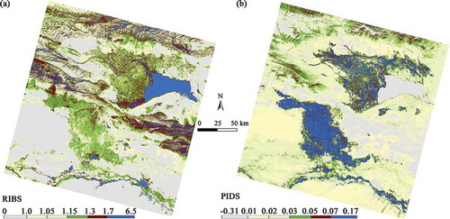
Figure 5. The boxplots of spectral indices of different land covers from Landsat 8 images: (a) RIBS; (b) PIDS.

Similar to the RIBS, the dark soil exhibited the smallest PIDS values (Figure 4(b)). Specifically, the averaged PIDS value from reference sites for dark soil was 0.008, with a standard derivation of 0.003. In contrast, other land covers except water body acquired higher PIDS values. The averaged PIDS values of grass, crop, and ISA were no less than 0.049. The PIDS can efficiently identify dark soil from other land covers except water body, which was also confirmed from the boxplots of PIDS values from reference sites (Figure 5(b)). The discrimination of water body could be implemented through combining the RIBS.

The bivariate density-sliced histogram plot between NNDSI_(3–6) and NTC1 also confirmed the separability of bright soil from other land covers including the vegetation (grass, crop, etc.), ISA, and water body (Figure 6(a)). Another bivariate density-sliced histogram plot between NDVI and TC1 was shown in Figure 6(b). These two spectral indices (NDVI and TC1) provided good discrimination between dark soil and other land covers such as ISA and vegetation. A simple threshold classification method could be applied to extract bright soil and dark soil due to the high distinctions.

Figure 6. Bivariate density-sliced histogram plots between (a) NNDSI (3–6) and NTC1, (b) NDVI and TC1.

4.1.2. Quantitative analysis of the RIBS and PIDS from Landsat 8 images

The spectral separability of RIBS indicated by SDI and JM distances between different land covers was provided in Table 1. The excellent separability between bright soil and other land covers was verified. The SDI value of RIBS between bright soil and other land covers (excluding dark soil) was consistently greater than 1.9. The SDI value of RIBS between bright soil and ISA, bright soil and water body was higher than 2.5. It revealed that RIBS can efficiently distinguish bright soil from ISA and water body. Good performance was also confirmed by the JM distances. The JM distances between bright soil and other land covers apart from dark soil were greater than 1.76. Specifically, the JM distance between bright soil and ISA was close to 2 (1.916), indicating perfect discrimination.

Table 1. SDI and JM distances of RIBS by Landsat image between different land covers.

SDI JM	Bright soil	Grass	Crop	ISA	Water	Dark soil
Bright soil		1.971	2.099	2.696	2.516	1.470
Grass	1.800		0.520	1.290	2.017	0.042
Crop	1.763	0.279		0.704	1.744	0.364
ISA	1.916	1.105	0.519		1.414	0.985
Water	1.874	1.589	1.555	1.246		1.829
Dark soil	1.369	0.170	0.181	0.763	1.598

Results from both SDI and JM distances indicated good spectral separability between dark soil and other land covers excluding the water and bright soil (Table 2). Specifically, the SDI of PIDS between dark soil and ISA, grass and crop was no less than 1.789, and the JM distances were greater than 1.64.

Table 2. Results of SDI and JM distance from PIDS between different land covers.

SDI JM	Dark soil	Grass	Crop	ISA	Water	Bright soil
Dark soil		1.924	2.366	1.789	0.151	1.075
Grass	1.732		0.216	0.252	1.143	1.222
Crop	1.837	0.878		0.493	1.373	1.57
ISA	1.642	0.191	1.189		1	1.011
Water	1.091	0.042	0.065	1.18		0.482
Bright soil	1.02	0.957	1.423	0.88	0.556

4.1.3. Comparative analysis with RNDSI

In order to calculate the RNDSI from Landsat image, a scatterplot between NDSI_(7–3) and TC1 is provided in Figure 7(a). The bright soil is distributed in the upper right corner and the water body in the bottom left corner of the scatterplot (Figure 7(a)). Other land covers including grass, crops, and ISA are scattered between them. Although the mean value of bright soil (1.145) was much lower than that from the ISA (1.419), their standard deviations were pretty high. The standard deviation of bright soil and ISA was 0.990 and 1.235, respectively. Large standard deviations of RNDSI were also found in other land covers (Figure 7(b)), which were often over 80% of the corresponding averaged values. The mean values of RNDSI from vegetation (grass and crop) were within bright soil and ISA and that from water body were higher than ISA (1.591). A mask of vegetation and water body was required in order to extract bright soil from ISA and the dark soil could not be separated (Figure 7(b)).

Figure 7. The scatterplot between (a) NDSI_(7–3) and TC1 and (b) boxplot of RNDSI of different land covers.

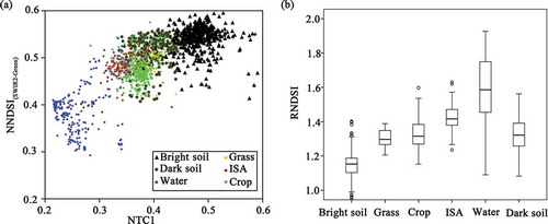
The performance assessments of RNDSI are provided in Table 3. The considerably good separability between bright soil and ISA was confirmed: the SDI value was 1.853 and the JM distance was 1.647. Although the SDI and JM distances were fairly lower than the proposed RIBS in this study, the performance of RNDSI was still good in separating bright soil from ISA. Nevertheless, the spectral separability of RNDSI between bright soil and vegetation (grass and crop) was not ideal, with the SDI and JM distances of less than 1.3. The dark soil could not be distinguished by RNDSI: the SDI and JM distances between dark soil and other land covers were consistently lower than 0.9.

Table 3. Results of SDI and JM distance from RNDSI between different land cover types.

SDI JM	Bright soil	Grass	Crop	ISA	Water	Dark soil
Bright soil		1.267	1.175	1.853	1.650	1.041
Grass	1.204		0.191	0.970	1.191	0.155
Crop	1.020	0.083		0.611	0.970	0.010
ISA	1.647	0.730	0.324		0.652	0.555
Water	1.518	1.090	0.862	0.618		0.914
Dark soil	0.893	0.331	0.018	0.339	0.762

4.2. Further applications to MODIS images

4.2.1. Spectral separability of the RIBS and PIDS from MODIS images

In order to evaluate the performances on images at different resolution and platforms, the two proposed soil indices (RIBS and PIDS) were further applied to MODIS images in China. The annual averaged spectral values free from cloud cover and snow in 2015 were utilized. The distribution map of RIBS (Figure 8 (a)) demonstrated the expected patterns: the bright soil in Northeast China consistently had the smallest values, water body and ISA exhibited very high values. From the spatial distribution map of PIDS, the dark soil exhibited very low values (Figure 8(b)). As confirmed from the boxplots of RIBS values of sampling sites (Figure 9), the RIBS values increased from bright soil, grass and sparse vegetation, crops, forests, ISA to water body, with mean values of 1.182, 1.628, 1.759, 2.196, 2.575, and 8.831, respectively. The mean PIDS value of dark soil, grass and sparse vegetation, crops, forests, and ISA was 0.024, 0.099, 0.181, 0.213, and 0.101, respectively (Figure 9).

Figure 8. Spatial distribution maps of (a) Ratio Index for Bright Soil and (b) Product Index for Dark Soil from MODIS images.

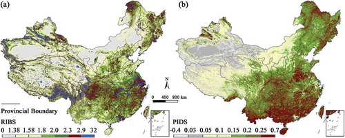
Figure 9. The boxplots of (a) RIBS and (b) PIDS for different land covers from MODIS images.

Quantitative analysis was performed by spectral separability (SDI and JM distance). The SDI values of RIBS between bright soil and other land covers (vegetation and ISA) were consistently higher than 1.3 (Table 4). The SDI value of RIBS between bright soil and ISA was around 2, indicating good discrimination between bright soil and ISA. Good spectral separability between bright soil and other land covers was also confirmed from the JM distance (Table 4). The JM distances between bright soil and other land covers were constantly greater than 1.37. In particular, the JM distance of RIBS between bright soil and ISA was 1.684. The SDI value of RIBS between bright soil and water body was only 1.031 due to the large variations within different water body across the whole county, and the JM distance was 1.733.

Table 4. The SDI and JM distances from RIBS estimated by MODIS images between different land covers.

SDI JM	Bright soil	Grass	Crop	Forest	ISA	Water	Dark soil
Bright soil		1.681	2.106	1.328	1.984	1.031	2.144
Grass	1.461		0.398	0.694	1.252	0.964	1.218
Crop	1.771	0.167		0.529	1.068	0.946	0.989
Forest	1.370	1.010	0.813		0.303	0.833	0.155
ISA	1.684	1.381	1.059	0.107		0.791	0.199
Water	1.733	1.663	1.665	1.228	1.333		0.833
Dark soil	1.767	1.170	0.914	0.049	0.162	1.421

The SDI values of PIDS between dark soil and other land covers were consistently higher than 1.5, except water and bright soil (Table 5). The JM distances between dark soil and other land covers (grass, crop, and ISA) were above 1.39. Performance assessments from both SDI and JM distance suggested good distinctions of dark soil from other land covers.

Table 5. Results of SDI and JM distance from PIDS between different land covers.

SDI JM	Dark soil	Grass	Crop	Forest	ISA	Water	Bright soil
Dark soil		1.552	2.789	3.821	1.595	0.322	1.205
Grass	1.402		0.995	1.513	0.02	0.302	0.708
Crop	1.901	0.69		0.389	0.982	0.858	1.912
Forest	1.998	1.399	0.128		1.502	1.138	2.713
ISA	1.395	0	0.796	1.335		0.314	0.739
Water	1.421	0.451	0.72	1.091	0.396		0.011
Bright soil	1.087	0.661	1.606	1.933	0.606	0.778

4.2.2. Classification accuracy of bare soil cover from MODIS images

Bright soil was classified by the RIBS using a simple threshold. Pixels with RIBS values less than 1.38 were identified as bright soil. Pixels with RIBS values greater than 2.9 were classified as water body. After water body was excluded, the dark soil was labeled when the PIDS values were less than 0.037. Accuracy assessment was conducted with reference sites (Table 6). Producer accuracy and user accuracy of bright and dark soil in 2015 was 94.96% and 91.88%, respectively. An overall accuracy of 94.00% was obtained when compared with the in-situ observation dataset. The kappa index was 0.8789. It verified that RIBS and PIDS could be utilized for classifying bright soil and dark soil covers.

Table 6. Accuracy assessments of MODIS-derived soil map in 2015 using reference data.

	Land cover
Reference data	Soil	Others	Producer accuracy (%)
Soil	735	39	94.96%
Others	65	894	93.22%
User accuracy (%)	91.88%	95.82%
Overall accuracy: 94.00%; Kappa: 0.8789

Counted in pixels.

4.2.3. Possible influences from snow cover

Given that both bright soil and snow cover exhibited high reflectance, it is necessary to exclude snow cover from bright soil. In order to evaluate the influence from snow cover, one 8-day composite MODIS image on February 17 was selected through a combined consideration of large snow coverage and minimum cloud cover. A total of 883,000 km² areas were identified as snow coverage from the MOD09A1 quality assessment layers, principally located in Northeast China and the Northern Xinjiang Province. The average value of the RIBS from snow coverage areas was 2.181, as opposed to 1.387 calculated from the reference sites of the bright desert. The standard deviation of snow cover and bright desert was 0.342 and 0.201, respectively. For snow cover and bright soil, the first and third interquartile ranged between 1.996–2.232 and 1.263–1.431, respectively. It is obvious that the bright soil obtained significantly lower values than those from snow cover. Good separability between snow cover and bright soil was also verified from the SDI and JM distance: the SDI was 1.4636 and the JM distance was 1.6264. If the bare soil areas were covered by snow, it would be identified as snow cover. Therefore, images free from cloud and snow cover should be selected and applied.

5. Discussion

5.1. Insights into designing spectral indices for different land surfaces

Developing soil indices is extremely challenging due to the soil spectral complexity and its confusion with ISA (Roberts et al. 2012; Deng et al. 2015). Till now, little work has been conducted in this field yet. Similar to vegetation and impervious surface indices, the major objective of developing soil indices is to derive a simple spectral enhancement approach that can highlight the contrasts among three major biophysical compositions following Ridd’s conceptual V–I–S model (Ridd 1995). This study characterized land surfaces based on the B–D–G model (Yue et al. 2014; Strahler, Woodcock, and Smith 1986; Kauth and Thomas 1976) and proposed two soil indices through these three dimensions.

The soil indices were designed to follow the mechanism of Ridd’s conceptual V–I–S triangle model (Ridd 1995). The scheme of the developed RIBS and PIDS was given in Figure 10. We borrowed the ideas of bright and dark ISA in developing the BCI for urban environment (Deng and Wu 2012). The complexity of soil spectral variability was incorporated through designing RIBS and PIDS for bright soil and dark soil, respectively. Through developing an index for bright soil (RIBS), the bright soil was expected to be distinguished by the smallest values; water was assumed to obtain the highest values (Figure 10). By proposing another index for dark soil (PIDS), it was expected that dark soil would be differentiated by the smallest values (Figure 10). Therefore, on the axis using the RIBS as the x-coordinate and PIDS as the y-coordinate, bright soil was located in the left corner (near coordinate origin) and the dark soil in the middle bottom (Figure 10). As far as we know, the PIDS was the only developed soil index that could distinguish dark soil from ISA.

Figure 10. The scheme of the developed RIBS and PIDS.

Optical remote sensing-based methods experienced an evolution from reflectance data, to vegetation indices (NDVI/EVI) and finally to combinations of multiple spectral indices (Dong and Xiao 2016). For example, a novel index for rice was successfully proposed based on EVI and Land Surface Water Index (Qiu et al. 2015). A BCI for remote sensing of urban environments was proposed through reexamining the three components from TC1 (Deng and Wu 2012). Another Novel Built-up Index was successfully developed based on three thematic indices: the Soil Adjusted Vegetation Index, the modified Normalized Difference Water Index, and the NDBI (Xu 2008). This study provided great insights into designing indicators based on three dimensions: brightness, darkness, and greenness. The spectral indices, TC1, NDSI, and NDVI, were selected to represent them (Becker and Choudhury 1988; Salomonson and Appel 2004; Baig et al. 2014; Zhang et al. 2002). Besides them, other spectral indices might also be utilized for this purpose. Compared with the former two dimensions (greenness and brightness), the dimension of darkness was seldom exploited for combined applications. The B–D–G model was often utilized in exploring urban landscape evolution. This study reinvestigated the B–D–G model in characterizing all land surfaces on Earth and illustrated its efficiency in developing soil indices for the purpose of improving land surface mapping accuracy. It was expected that this study would provide valuable thinking into developing effective indices from various dimensions.

5.2. Geographic understanding of the developed soil indices

The developed RIBS has noteworthy meaning for land use/cover research community due to its significant negative association with proportions of bare bright soil coverage. The water bodies had extremely high values and the ISA also acquired high values. The soil fractional coverage of water bodies and ISA is the least among all land covers. When the land surface is covered by permanent water bodies or ISA, it is less likely that the bare soil would be exposed since ISA are compact and permanent all year-round (Carrion-Flores and Irwin 2004). Vegetation gained medium RIBS values, increasing from grass and agricultural crops to forest cover. For land cover of vegetation, it is often a mixture of vegetation and bare soil depending on the vegetation types, its density, and climatic regions. Forests generally have longer vegetation coverage compared with other vegetation (Qiu, Liu et al. 2016). Agricultural crops commonly exhibited stronger vegetation density compared with grass (Qiu et al. 2013). The proportions of bare soil often declined when land cover changed from grass and agricultural crops to forests due to the usually longer growing length of forests (Qiu, Wang et al. 2016). The bare bright soil achieved the smallest RIBS values. Therefore, the proposed RIBS successfully separate bright soil (including sand), vegetation, ISA, and water bodies. The RIBS could be regarded as an indication of land surface bareness, with lower values reflecting distinct bareness.

5.3. Significances and advantages of the developed soil indices

The developed soil indices will promote and accelerate the developments of impervious spectral indices through their combined applications. Separating soil from ISA is an important mission for impervious spectral indices (Xu 2010; As-Syakur, Adnyana, and Nuarsa 2012; Deng and Wu 2012; Zha, Gao, and Ni 2003). Existing impervious indices such as the NDBI failed in this mission (Deng and Wu 2012). Therefore, preprocessing to remove soil and water is often needed in many methods due to the confusion with impervious surfaces (Xu 2010). In contrast to those existing impervious indices, it is interesting and remarkable that the developed RIBS achieved greater separability between soil and ISA compared with between soil/ISA and others (e.g., grass, crops, and forest). Consequently, it was assumed that the developed RIBS could further be applied to distinguish impervious surface through its combinations with vegetation indices and PIDS.

The developed soil indices verified its robust capacity in separating bright and dark soils from the complexity of different land covers and disturbances from background noise. In the developed RIBS, no preprocessing work is required to mask out background noise such as water body and vegetation. Even both with high reflectance, the developed RIBS could efficiently discriminate bright soil from snow cover. Therefore, it holds easy applications to multiple categories of images in a large area without relying on secondary data.

In all, the proposed soil indices were proved to be efficient in distinguishing soil cover through the applications on both MODIS and Landsat images. The developed RIBS in this study achieved better separability compared with the recently proposed soil index (Deng et al. 2015). There was no spectral index which could highlight dark soil from other land covers yet. This study fills the gap through developing the PIDS. Nevertheless, it should be noted that the RNDSI (Deng et al. 2015) made a significant contribution to the research fields of designing spectral indices. Our study improved the soil index proposed by Deng et al. (2015) to enhance separability between multiple land covers such as bright soil, dark soil, ISA, water body, and vegetation.

5.4. Prospects and future works

Although application results suggested that the developed RIBS can be utilized as an indication of soil abundance across all land covers regarding its density and durations, it is difficult to provide a rigorous validation due to the difficulty of deriving ground truth soil fractures in the study area (Deng and Wu 2012). The ability of RIBS to separate small areas of bare soil located in vegetation and ISA has not been widely certified yet. As an empirical strategy, the effectiveness of the proposed RIBS and PIDS needs to be further evaluated with a large variety of different images (i.e., SPOT, worldview, QuickBird) from regional to global scales.

Future work could be conducted in the following aspects. First, the rational and mechanisms of these developed soil indices would be further investigated and evaluated. Whether other land surface such as the impervious surface could be distinguished by bright and dark impervious surfaces through this strategy? Second, other spectral indices representing the dimensions of greenness, brightness, and darkness could be explored in the calculations of these soil indices. Third, some modifications could be applied if we want to obtain positive relationships between bright/dark soil and RIBS/PIDS. Compared with vegetation and ISA, the bright/dark soil obtained significantly the smallest values in the proposed RIBS/PIDS. Finally, further applications and validations on other images and other regions could be conducted.

6. Conclusions

The spatial distribution of soil, vegetation, and ISA are indispensable for understanding the land cover dynamic process. Compared with spectral indices for vegetation, the development of soil and ISA indices is more challenging due to the complexity of soil/ISA spectra and their difficulty in separating soil and ISA. This paper developed two soil indices in order to extract bright/dark soil cover from vegetation, ISA, and water. Performance assessments suggest that the bright soil index is capable of distinguishing bright soil from ISA without masking vegetation and water body. The developed bright soil index can be applied to both Landsat and the MODIS images to delineate the distribution of bright soil. Similarly, the other soil index for dark soil can be easily applied to extract dark soil due to the consistently smallest values.

The developed soil indices in this paper have the following advantages. First, the developed two soil indices have reliable performance with regard to spectral separability and classification accuracy. Second, the developed RIBS can distinguish bright soil without using the masks of vegetation and water body. It can be utilized straightforward with little preprocessing work. Third, the developed RIBS can be utilized as an indication of surface bareness, increasing from bare bright soil and vegetation to ISA and water body. Fourth, the bright soil and snow cover can be distinguished by the developed RIBS, although both have high reflectance. Fifth, the dark soil, which was often neglected, can be extracted by the established PIDS. Finally, the developed soil indices can be applied to various remote sensing images at different spectral and spatial resolutions.

Acknowledgements

This work was supported by the National Natural Science Foundation of China (grant no. 41471362) and funding from the Science Bureau of Fujian Province (2017I0008).

Disclosure statement

No potential conflict of interest was reported by the authors.

Additional information

Funding

This work was supported by the National Natural Science Foundation of China: [Grant Number 41471362].

References

- As-Syakur, A. R., I. Adnyana, and I. W. Nuarsa. 2012. “Enhanced Built-Up and Bareness Index (EBBI) for Mapping Built-Up and Bare Land in an Urban Area.” Remote Sensing 4 (10): 2957–2970. doi:10.3390/rs4102957.
- Baig, M. H. A., L. Zhang, T. Shuai, and Q. Tong. 2014. “Derivation of a Tasselled Cap Transformation Based on Landsat 8 At-Satellite Reflectance.” Remote Sensing Letters 5 (5): 423–431. doi:10.1080/2150704X.2014.915434.
- Becker, F., and B. J. Choudhury. 1988. “Relative Sensitivity of Normalized Difference Vegetation Index (NDVI) and Microwave Polarization Difference Index (MPDI) for Vegetation and Desertification Monitoring.” Remote Sensing of Environment 24 (2): 297–311. doi:10.1016/0034-4257(88)90031-4.
- Ben-Dor, E. 2002. “Quantitative Remote Sensing of Soil Properties.” Advances in Agronomy 75: 173–243.
- Carrion-Flores, C., and E. G. Irwin. 2004. “Determinants of Residential Land-Use Conversion and Sprawl at the Rural-Urban Fringe.” American Journal of Agricultural Economics 86 (4): 889–904. doi:10.1111/j.0002-9092.2004.00641.x.
- Deng, C., and C. Wu. 2012. “BCI: A Biophysical Composition Index for Remote Sensing of Urban Environments.” Remote Sensing of Environment 127: 247–259. doi:10.1016/j.rse.2012.09.009.
- Deng, Y., W. Changshan, L. Miao, and R. Chen. 2015. “RNDSI: A Ratio Normalized Difference Soil Index for Remote Sensing of Urban/Suburban Environments.” International Journal of Applied Earth Observation and Geoinformation 39: 40–48. doi:10.1016/j.jag.2015.02.010.
- Dong, J., and X. Xiao. 2016. “Evolution of Regional to Global Paddy Rice Mapping Methods: A Review.” ISPRS Journal of Photogrammetry and Remote Sensing 119: 214–227. doi:10.1016/j.isprsjprs.2016.05.010.
- Ellis, E., and R. Pontius. 2007. “Land-Use and Land-Cover Change.” In Encyclopedia of Earth, edited by C. J. Cleveland. Washington, DC: Environmental Information Coalition, National Council for Science and the Environment.
- Gómez, C., J. C. White, and M. A. Wulder. 2016. “Optical Remotely Sensed Time Series Data for Land Cover Classification: A Review.” Isprs Journal of Photogrammetry and Remote Sensing 116: 55–72. doi:10.1016/j.isprsjprs.2016.03.008.
- Guo, Z., and S. Du. 2017. “Mining Parameter Information for Building Extraction and Change Detection with Very High-Resolution Imagery and GIS Data.” Giscience & Remote Sensing 54 (1): 38–63. doi:10.1080/15481603.2016.1250328.
- Huete, A., K. Didan, T. Miura, E. P. Rodriguez, X. Gao, and L. G. Ferreira. 2002. “Overview of the Radiometric and Biophysical Performance of the MODIS Vegetation Indices.” Remote Sensing of Environment 83 (1–2): 195–213. doi:10.1016/S0034-4257(02)00096-2.
- Jiang, Z., A. R. Huete, K. Didan, and T. Miura. 2008. “Development of a Two-Band Enhanced Vegetation Index without a Blue Band.” Remote Sensing of Environment 112 (10): 3833–3845. doi:10.1016/j.rse.2008.06.006.
- Kauth, R. J., and G. S. Thomas. 1976. “The Tasselled Cap–A Graphic Description of the Spectral-Temporal Development of Agricultural Crops as Seen by Landsat.” Paper presented at the LARS Symposia. Symposium on Machine Processing of Remotely Sensed Data, Purdue University, West Lafayette, IN, June 29-July 1, 1976
- Liu, J., M. Liu, D. Zhuang, Z. Zhang, and X. Deng. 2003. “Study on Spatial Pattern of Land-Use Change in China during 1995–2000.” Science in China Series D: Earth Sciences 46 (4): 373–384. doi:10.1360/03yd9033.
- Lõhmus, K., T. Oja, and R. Lasn. 1989. “Specific Root Area: A Soil Characteristic.” Plant and Soil 119 (2): 245–249. doi:10.1007/BF02370415.
- Müller, H., P. Griffiths, and P. Hostert. 2016. “Long-Term Deforestation Dynamics in the Brazilian Amazon—Uncovering Historic Frontier Development along the Cuiabá–Santarém Highway.” International Journal of Applied Earth Observation and Geoinformation 44: 61–69. doi:10.1016/j.jag.2015.07.005.
- Qiu, B., Z. Liu, Z. Tang, and C. Chen. 2016. “Developing Indices of Temporal Dispersion and Continuity to Map Natural Vegetation.” Ecological Indicators 64: 335–342. doi:10.1016/j.ecolind.2016.01.006.
- Qiu, B., Z. Wang, Z. Tang, C. Chen, Z. Fan, and L. Weijiao. 2016. “Automated Cropping Intensity Extraction from Isolines of Wavelet Spectra.” Computers and Electronics in Agriculture 125: 1–11. doi:10.1016/j.compag.2016.04.015.
- Qiu, B., L. Weijiao, Z. Tang, C. Chen, and Q. Wen. 2015. “Mapping Paddy Rice Areas Based on Vegetation Phenology and Surface Moisture Conditions.” Ecological Indicators 56: 79–86. doi:10.1016/j.ecolind.2015.03.039.
- Qiu, B. W., Z. L. Fan, M. Zhong, Z. H. Tang, and C. C. Chen. 2014. “A New Approach for Crop Identification with Wavelet Variance and JM Distance.” Environmental Monitoring and Assessment 186:7929–40. doi:10.1007/s11769-013-0649-y.
- Qiu, B. W., C. Y. Zeng, Z. H. Tang, and C. C. Chen. 2013. “Characterizing Spatiotemporal Non-Stationarity in Vegetation Dynamics in China Using MODIS EVI Dataset.” Journal of Environmental Monitoring and Assessment 185 (11): 9019–9035. doi:10.1007/s10661-013-3231-2.
- Radeloff, V. C., D. J. Mladenoff, and M. S. Boyce. 1999. “Detecting Jack Pine Budworm Defoliation Using Spectral Mixture Analysis: Separating Effects from Determinants.” Remote Sensing of Environment 69 (2): 156–169. doi:10.1016/S0034-4257(99)00008-5.
- Ren, Y., L. Xin, L. Ling, and L. Zengyuan. 2012. “ Large-Scale Land Cover Mapping with the Integration of Multi-Source Information Based on the Dempster-Shafer Theory.” International Journal of Geographical Information Science 26 (1): 169–191. doi:10.1080/13658816.2011.577745.
- Ridd, M. K. 1995. “Exploring a VIS (Vegetation-Impervious Surface-Soil) Model for Urban Ecosystem Analysis through Remote Sensing: Comparative Anatomy for Cities†.” International Journal of Remote Sensing 16 (12): 2165–2185. doi:10.1080/01431169508954549.
- Roberts, D. A., D. A. Quattrochi, G. C. Hulley, S. J. Hook, and R. O. Green. 2012. “Synergies between VSWIR and TIR Data for the Urban Environment: An Evaluation of the Potential for the Hyperspectral Infrared Imager (Hyspiri) Decadal Survey Mission.” Remote Sensing of Environment 117: 83–101. doi:10.1016/j.rse.2011.07.021.
- Salomonson, V. V., and I. Appel. 2004. “Estimating Fractional Snow Cover from MODIS Using the Normalized Difference Snow Index.” Remote Sensing of Environment 89 (3): 351–360. doi:10.1016/j.rse.2003.10.016.
- Sheppard, S. R. J., and P. Cizek. 2009. “The Ethics of Google Earth: Crossing Thresholds from Spatial Data to Landscape Visualisation.” Journal of Environmental Management 90 (6): 2102–2117. doi:10.1016/j.jenvman.2007.09.012.
- Strahler, A. H., C. E. Woodcock, and J. A. Smith. 1986. “On the Nature of Models in Remote Sensing.” Remote Sensing of Environment 20 (2): 121–139. doi:10.1016/0034-4257(86)90018-0.
- Van Niel, T. G., T. R. McVicar, and B. Datt. 2005. “On the Relationship between Training Sample Size and Data Dimensionality: Monte Carlo Analysis of Broadband Multi-Temporal Classification.” Remote Sensing of Environment 98 (4): 468–480. doi:10.1016/j.rse.2005.08.011.
- Wardlow, B. D., S. L. Egbert, and J. H. Kastens. 2007. “Analysis of Time-Series MODIS 250 M Vegetation Index Data for Crop Classification in the US Central Great Plains.” Remote Sensing of Environment 108 (3): 290–310. doi:10.1016/j.rse.2006.11.021.
- Xu, H. 2008. “A New Index for Delineating Built‐Up Land Features in Satellite Imagery.” International Journal of Remote Sensing 29 (14): 4269–4276. doi:10.1080/01431160802039957.
- Xu, H. 2010. “Analysis of Impervious Surface and Its Impact on Urban Heat Environment Using the Normalized Difference Impervious Surface Index (NDISI).” Photogrammetric Engineering & Remote Sensing 76 (5): 557–565. doi:10.14358/PERS.76.5.557.
- Yang, X., K. Zhang, B. Jia, and L. Ci. 2005. “Desertification Assessment in China: An Overview.” Journal of Arid Environments 63 (2): 517–531. doi:10.1016/j.jaridenv.2005.03.032.
- Yue, W., Y. XinYue, X. Jianhua, X. Lihua, and J. Lee. 2014. “A Brightness–Darkness–Greenness Model for Monitoring Urban Landscape Evolution in a Developing Country – A Case Study of Shanghai.” Landscape and Urban Planning 127: 13–17. doi:10.1016/j.landurbplan.2014.04.010.
- Zha, Y., J. Gao, and S. Ni. 2003. “Use of Normalized Difference Built-Up Index in Automatically Mapping Urban Areas from TM Imagery.” International Journal of Remote Sensing 24 (3): 583–594. doi:10.1080/01431160304987.
- Zhang, X., C. B. Schaaf, M. A. Friedl, A. H. Strahler, G. Feng, and J. C. F. Hodges. 2002. “MODIS Tasseled Cap Transformation and Its Utility.” Paper presented at the Geoscience and Remote Sensing Symposium, 2002. IGARSS ‘02. 2002 IEEE International, 24–28 June 2002. Toronto: IEEE.
- Zhu, Z., and C. E. Woodcock. 2014. “Automated Cloud, Cloud Shadow, and Snow Detection in Multitemporal Landsat Data: An Algorithm Designed Specifically for Monitoring Land Cover Change.” Remote Sensing of Environment 152: 217–234. doi:10.1016/j.rse.2014.06.012.