Building block level urban land-use information retrieval based on Google Street View images

Abstract

Land-use maps are important references for urban planning and urban studies. Given the heterogeneity of urban land-use types, it is difficult to differentiate different land-use types based on overhead remotely sensed data. Google Street View (GSV) images, which capture the façades of building blocks along streets, could be better used to judge the land-use types of different building blocks based on their façade appearances. Recently developed scene classification algorithms in computer vision community make it possible to categorize different photos semantically based on various image feature descriptors and machine-learning algorithms. Therefore, in this study, we proposed a method to derive detailed land-use information at building block level based on scene classification algorithms and GSV images. Three image feature descriptors (i.e., scale-invariant feature transform-Fisher, histogram of oriented gradients, GIST) were used to represent GSV images of different buildings. Existing land-use maps were used to create training datasets to train support vector machine (SVM) classifiers for categorizing GSV images. The trained SVM classifiers were then applied to case study areas in New York City, Boston, and Houston, to predict the land-use information at building block level. Accuracy assessment results show that the proposed method is suitable for differentiating residential buildings and nonresidential buildings with an accuracy of 85% or so. Since the GSV images are publicly accessible, this proposed method would provide a new way for building block level land-use mapping in future.

Keywords:

• GSV (Google Street View)
• machine learning
• image features
• urban land-use mapping

1. Introduction

The land-use change is a reflection of human activities on land to change its physical cover, ecosystem service, and social functions (Tayyebi et al. 2014; Meehan et al. 2013). The land-use change is the root cause of many environmental, ecological, and social issues (Tayyebi, Pijanowski, and Pekin 2015). Detailed knowledge of land-use change is very important for sustainable planning (Tayyebi et al. 2014).

Traditionally, overhead remotely sensed data are widely used for land-cover/use mapping. Different types of land cover/use usually show different spectral characteristics (Blaschke 2010; Myint et al. 2011) in overhead view remotely sensed imagery, which makes it possible to classify different land-cover/use types based on remotely sensed data. Proliferating image processing algorithms have been developing to differentiate different land-use types from remotely sensed data. Many machine-learning classifiers were applied to land-cover/use mapping based on the remotely sensed data, such as, maximum likelihood classifier (Jensen 2005; Frohn et al. 2011; Li et al. 2013), support vector machine (SVM) (Vapnik 1995; Mountrakis, Im, and Ogole 2011; Xun and Wang 2015; Lin and Yan 2016; Chu et al. 2016), and artificial neural network (Bruzzone and Prieto 1999), etc. The object-based image analysis was also proposed to differentiate different land-cover/use types based on remotely sensed images (Definiens 2008; Blaschke 2010; Myint et al. 2011). The object-based classification method usually first segment remotely sensed images into different objects, which are further categorized into different land-cover/use types based on their spectral and geometrical characteristics (Li et al. 2013). The object-based classification method has been proved to increase the accuracy of the classification results significantly (Hussain and Shan 2016; Qiu, Wu, and Miao 2014; Wang et al. 2016). Other than algorithm development, prior knowledge of the land-use change was also incorporated in generating land-use maps (Ray and Pijanowski 2010; Tayyebi, Pijanowski, and Pekin 2015). Based on the prior knowledge of the historic and future shift in landscape, it is possible to create land-use map for future and past (Tayyebi, Pijanowski, and Pekin 2015).

High-resolution urban land-use maps are important references for studies of urban shrinkage and sprawl (Haase et al. 2012; Gennaio, Hersperger, and Bürgi 2009), urban population mapping (Ural, Hussain, and Shan 2011; Lwin and Murayama 2009), etc. However, urban land-use classes are heterogeneous, and different land-use types may have similar spectral signatures and spatial patterns. In addition, remotely sensed data only capture the overhead view of urban features, which may further influence land-use mapping results. For example, the overhead view of remotely sensed data only captures the spectral reflectance of building roofs, which can hardly reflect the different social functions or land-use types of buildings. The existing of roof garden and different roof pavements will cause misclassification.

Recently, with the availability of geo-tagged civic data, new methods have been developed for land-use mapping based on the social function information derived from civic data (Thomas et al. 2014; Liu et al. 2016; Hu et al. 2016). These civic data include cell phone call data (Soto and Frias-Martinez 2011a; Soto and Frias-Martinez 2011b), geo-located social media data (Leung and Newsam 2012; Hu et al. 2016), and taxi trajectory data (Liu et al. 2016). Considering the fact that different land-use types may have different social functions, it is reasonable to judge the land-use types of different regions in cities based on their social function information. For example, residential areas are places for people to live but commercial areas are places for people to work. The cell phone call data and taxi trajectory data allow us to infer where people live and work, which may further help to infer land-use information. The major issue faced by application of the civic data is that the civic data are usually not publicly available. These civic data also bring some other concerns for urban land-use mapping, such as social and spatial bias, potential privacy violation, and relatively coarse resolution. All of these issues would further influence the applications of civic data for land-use mapping.

New methods are in need for high-resolution land-use mapping without much data limitation. Different from the overhead remotely sensed data, Google Street View (GSV) images capture the profile views of cityscapes, which provide us a new data source for urban studies at a very different perspective (Li et al. 2015). Since representing the ground truth at a very high resolution, GSV images have been widely used as references for validating land-cover/use mapping results in previous studies. The profile view of street-level images could better be used to judge the land-use types of different building blocks (Li and Zhang 2016). Considering the dense coverage of GSV panoramas in cities, GSV could become a new data source for generating fine-level land-use maps, especially for urban areas. This study applied scene classification algorithms for land-use mapping based on GSV images and verified the extendibility of the method for land-use mapping in different cities with different environments.

2. Related work

Scene categorization or scene classification is the fundamental problem in the computer vision field (Xiao et al. 2010). In the past decade, advancement in computer vision makes it possible to categorize or classify images semantically. Large databases of different scene images together with the corresponding scene category labels were built for scene recognition. Caltech-101 dataset (Fei-Fei, Fergus, and Perona 2004) is one of the first standardized datasets for multi-category image classification, with 101 object classes and commonly 15–30 training images per class. Xiao et al. (2010) built the Scene UNderstanding (SUN) database for classifying various images. The SUN dataset was built to cover as many different scenes as possible, and it covers 899 categories and 130,519 images (Xiao et al. 2010). Since 2010, the ImageNet Large Scale Visual Recognition Challenge (ILSVRC) was launched to motivate the computer vision community to make progress on large-scale scene classification. Participants join this competition to compare their scene classification algorithms based on the ImageNet database.

In recent years, scene classification methods have been applied to land-use classification. Scene classification methods were first applied to overhead view remotely sensed imagery for land-use information retrieval (Xu et al. 2010; Yang and Newsam 2010; Yang and Newsam 2013; Zhao et al, 2016a, 2016b). Different image features computed based on the color and texture of remotely sensed images are commonly used to represent images and train image classifiers (Yang and Newsam 2010; Yang and Newsam 2013). Xu et al. (2010) proposed to use Bag-of-Visual Words (BOV) to bridge the semantic gap between low-level image features and high-level land-use concepts. Results show that the BOV helps to increase the accuracy of the classification results significantly. Yang and Newsam (2013) used the local invariant features calculated from high-resolution aerial imagery to retrieval land-use information. Results show that the performance of the local invariant features varies on different land-use types. Although overhead remotely sensed data have been widely used to map land-cover types, it is more difficult to distinguish different land-use types (Leung and Newsam 2012). This is because different from land cover, which represents the natural landscape, land use shows the social function of the landscape. It is difficult to recognize the social functions of landscapes based on the spectral signatures and spatial patterns represented in the overhead remotely sensed data. In order to complement the shortcoming of remotely sensed data for land-use mapping, Leung and Newsam (2012) explored how to use the geo-referenced Flickr images for land-use classification. Each downloaded Flickr image was labeled to a ground truth land-use type based on the existing land-use map. The image feature – Bag of visual Words – was first calculated for each image. SVMs were then trained based on the calculated image feature vectors and labels to assign land-use labels to the test images based on their image feature vectors.

There are still few scene classification studies based on street level images in literature. Salesses, Schechtner, and Hidalgo (2013) collected 2920 GSV images in New York City and Boston and labeled those images with different perceptual attributes via a crowdsourcing website – Place Pulse. Based on the Place Pulse dataset, Naik et al. (2014) trained a prediction model to map the safety perception in a couple of American cities using machine-learning and image feature extraction approaches. Li et al. (2015) verified the possibility of using GSV images to study the visibility of street greenery in New York City using an image classification algorithm. Li and Zhang (2016) demonstrated the potential of using GSV images for land-use mapping in a very small area of New York City. However, cross-validation was not conducted and the extendibility of the method was not tested.

Computation of image features based on the color and texture of images is a requisite step in scene classification. Proliferating image features were proposed to describe and represent scene images for scene categorization (Xiao et al. 2010). The most popular image features include GIST (Oliva and Torralba 2001), histogram of oriented gradients (HoG) (Dalal and Triggs 2005; Felzenszwalb et al. 2010), scale-invariant feature transform descriptors (SIFT), self-similarity descriptors (Shechtman and Irani 2007), and deep convolutional activation features (Donahue et al. 2013).

3. Materials and methods

3.1. Study area and data

Case study areas were selected from New York City, Boston, and Houston in this study (Figure 1(a)), because of the availability of various spatial data and the dense coverage of GSV images in these three cities.

Figure 1. (a) The locations of the study areas and land-use map of a case study area in New York City and (b) the land-use classification system in this study. For full colour versions of the figures in this paper, please see the online version.

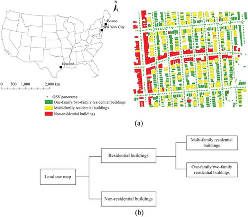
The building footprint maps and land-use maps in the study areas were downloaded from different city governments’ websites. The original land-use classification system was first aggregated into three major types: one-family/two-family residential buildings, multifamily residential buildings, and nonresidential buildings (Figure 1(b)). The original land-use maps are at parcel level. Since the study is focused on recognizing land-use types of different building blocks, therefore, the original land-use maps were overlapped with the building footprint maps to generate building block level land-use maps. Figure 1(a) shows a generated building block level land-use map in the case study area of New York City.

The proposed land-use mapping method is based on a three-step workflow (Figure 2). First, GSV images capturing façades of building blocks along streets were collected and labeled based on the existing land-use maps. Our approach does not require individual GSV images to be manually labeled. Then, the dataset with GSV images and land-use labels were split into training set and testing set. Three image features, GIST, HoG, and scale-invariant feature transform-Fisher (SIFT-Fisher) vectors, were calculated and compared for all GSV images in the training set to train SVM classifiers. Finally, accuracy assessment was conducted on the testing set to validate the classification results of those trained SVM classifiers.

Figure 2. The workflow of the proposed method.

3.2. Linking GSV images to building blocks

GSV images capture the profile view of building blocks along streets. By setting appropriate parameters in GSV static Image API, it is possible to get the GSV image covering the façade of a specific building block (Li and Zhang 2016).

Figure 3(a) shows the geometrical model between the footprint of a building block and its nearby GSV site (G_x, G_y). The field of view (fov) angle can be calculated by the following equation:

(1) $fov=arccos\left(\frac{{\mathrm{V}}_1\cdot {\mathrm{V}}_2}{||{\mathrm{V}}_1\left|\left|\times \right|\right|{\mathrm{V}}_2||}\right)$(1)

Figure 3. Geometrical model for choosing optimum heading and fov to represent façades of building blocks.

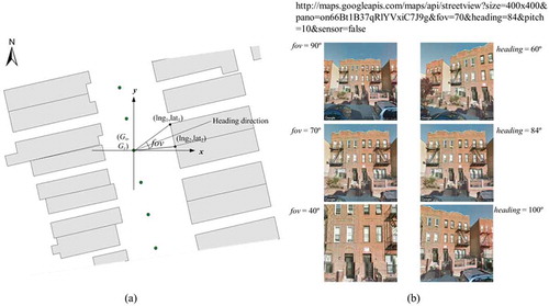
In above equation, the vectors V₁ and V₂ are

${\mathrm{V}}_1=\left(ln{g}_1-G_x,la{t}_1-G_y\right),$

${\mathrm{V}}_2=\left(ln{g}_2-\hspace{0.17em}{G}_x,la{t}_2-G_y\right)$

where (lng₁, lat₁) and (lng₂, lat₂) are the coordinates of two endpoints of a building façade. Based on previous study (Li and Zhang 2016), we set the maximum and minimum thresholds of fov as 90 and 30 to decrease distortion in the static GSV images and make sure GSV images capturing patterns in building façades, respectively. The heading angle heading was set as the heading direction, and ranges from 0 to 360. Figure 3(b) shows six static GSV images of one site with the panorama ID “on66Bt1B37qRlYVxiC7J9g” with different heading angles and field of view angles.

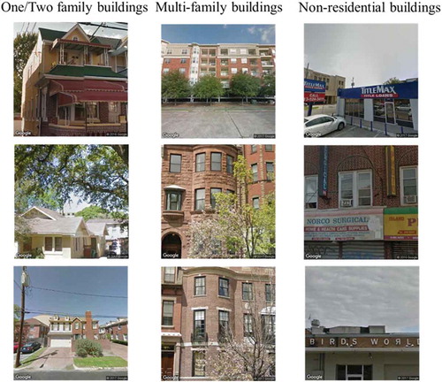
Based on the geometric model, for each building block, we selected the closest panorama for the GSV image collection by specifying the corresponding heading and fov parameters. Each GSV image was then labelled to the land-use type of that building block. Figure 4 shows several collected GSV images with their corresponding land-use types in the study area.

Figure 4. Buildings blocks with different land-use types on street level images.

3.3. Image feature extraction

Image features, which are calculated based on the spectral and geometrical information in images, are key to derive land-use information from images. Three commonly used generic image features (GIST, HoG, and SIFT-Fisher) were used in this study to represent and classify GSV images.

3.3.1. GIST

The GIST is typically computed over the entire image (i.e., it is a global image descriptor) to represent the perceptual properties of a scene (naturalness, openness, roughness, expansion, and ruggedness) for the purpose of scene classification. The GIST summarizes the orientations and scales, both of which provide a rough description of an image, for different parts of the image. The GIST was originally proposed for scene categorization, and it represents both the low-level image features and the layout of images without any form of segmentation (Oliva and Torralba 2001). The GIST of a given image is usually computed in three steps:

Step 1. Convolve the image with Gabor-like filters tuned to 4 scales and 8 orientations to produce 32 feature maps of the same size of the input image. The parameters of these filters were determined based on different types of scene pictures to represent the naturalness, openness, roughness, expansion, and ruggedness of scene.

Step 2. Divide each feature map into 16 regions (by a 4 × 4 grid) and then average the feature values within each region.

Step 3. Concatenate the averaged feature values of all 32 feature maps (16 per feature map), thus resulting in a 512 (i.e., 16 × 32) GIST descriptor.

Please see Oliva and Torralba (2001) for more details about the computation of GIST feature.

3.3.2. HoG descriptor

The HoG descriptor is a feature descriptor widely used to detect objects in the computer vision field. In order to calculate the HoG descriptor for GSV images, each image is first divided into 8 × 8 squared cells and the gradients are calculated for each cell using 1D [−1, 0, 1] masks. The gradient vector, orientation, and magnitude of an image f are calculated using the following equations,

(2) $\mathrm{g}\mathrm{r}\mathrm{a}\mathrm{d}(f)=\left(\frac{\mathrm{\partial }f}{\mathrm{\partial }x},\frac{\mathrm{\partial }f}{\mathrm{\partial }y}\right)$(2)

where $\partial f/\partial x\approx \left(1/2\right)[f(x+1,y)-f(x-1,y)],\partial f/\partial y\approx \left(1/2\right)[f(x,y+1)-f(x,y-1)].$ The orientation and the magnitude can be calculated as,

(3) $\mathrm{o}\mathrm{r}\mathrm{i}\mathrm{e}\mathrm{n}\mathrm{t}\mathrm{a}\mathrm{t}\mathrm{i}\mathrm{o}\mathrm{n}(\mathrm{g}\mathrm{r}\mathrm{a}\mathrm{d}(f))={tan}^{-1}\left(\frac{\mathrm{\partial }f}{\mathrm{\partial }y}/\frac{\mathrm{\partial }f}{\mathrm{\partial }x}\right)$(3)

(4) $\mathrm{m}\mathrm{a}\mathrm{g}\mathrm{n}\mathrm{i}\mathrm{t}\mathrm{u}\mathrm{d}\mathrm{e}(\mathrm{g}\mathrm{r}\mathrm{a}\mathrm{d}(f))=\sqrt{\frac{\mathrm{\partial }{f}^2}{\mathrm{\partial }x}+\frac{\mathrm{\partial }{f}^2}{\mathrm{\partial }y}}$(4)

A histogram of gradients is then created using a block-wise pattern for each cell. The bins of the histogram are defined by gradient orientations, ranging from 0 to 180 degrees or 0 to 360 degrees. Previous studies have showed that setting the bins space over 0–180 degrees is more suitable for human detection (Dalal and Triggs 2005). Therefore, in this study, we set the bins range from 0 to 360 degrees. The number of orientation bins is usually set to 9 because of its good performance. Each gradient’s contribution to the histogram is split between the two nearest bins, and it is equal to its magnitude. The histograms of gradients are further normalized to make the HoG descriptor insensitive to shadows and different illumination conditions. Then, histograms of gradients of all four 2 × 2 neighboring cells are concatenated into one giant vector descriptor – HoG. The concatenated descriptors are spatially overlapped, because higher feature dimensionality provides more descriptive power (Dalal and Triggs 2005; Xiao et al. 2010). In this study, the HoG was calculated based on an online code provided by Felzenszwalb et al. (2010).

3.3.3. SIFT-Fisher vector

The SIFT descriptor proposed by Lowe (2004) is based on one of the most popular image feature – SIFT, which has been widely used for scene classification, solving 3D structure from multiple images, and motion tracking. The SIFT descriptor is invariant to illumination changes, scaling, rotation, and minor changes in viewing direction, which together make it promising for static GSV image classification.

The first step of computing the SIFT descriptor is to detect the scale-space extremes of an image. An image I (x, y) is first blurred by a Gaussian function using the following equation,

(5) $\begin{array}{c}L=G\ast I\\ L(x,y,\sigma )=\sum _{u=-n}^n\sum _{v=-n}^{n}G(u,v,\sigma )I(x-u,y-v)\end{array}$(5)

where L is the blurred image, * is the convolution operation, n is the size of the Gaussian kernel, and G is the Gaussian function,

(6) $G(u,v,\sigma )=\frac{1}{2\pi {\sigma }^2}{e}^{-\left(u^2+v^2\right)/2{\sigma }^2}$(6)

In order to increase the time efficiency, Difference-of-Gaussians (DoG) function is used to locate the scale-space extreme. The DoG is computed as,

(7) $D\left(x,y,\sigma \right)=L\left(x,y,k\sigma \right)-L\left(x,y,\sigma \right)$(7)

The local maxima and minima of D(x, y, σ) are located by comparing each point with its 26 neighbors, which include 8 neighbors at the same scale and 9 neighbors up and down one scale. If this value is the minimum or maximum of all these points, then this point is an extreme. Taylor expansion is further applied on the DoG function to locate SIFT keypoints. The key points are located by taking the derivative of this function with respect to x, y and setting it to zero (Lowe 2004).

In order to decrease the noise in the detected keypoints information, the initial extreme points are further refined by removing low contrast extreme points and eliminating the edge response. Those low contrast keypoints can be eliminated by setting threshold on the DoG function directly. This method is not suitable to eliminate those keypoints along the edge, because the DoG function will have a strong response along edges. However, those keypoints along the edge have large principal curvatures across the edge but small principal curvatures in the perpendicular direction. Based on this, a 2 × 2 Hessian matrix can be used to remove the outlier keypoints. The Hessian matrix is computed based on the derivatives of DoG function at different directions as,

(8) $H=\left[\begin{array}{cc}{D}_{xx}& D_{xy}\\ D_{xy}& D_{yy}\end{array}\right]$(8)

(9) $\frac{Tr{(H)}^2}{Det(H)}<\frac{{\left(r_0+1\right)}^2}{r_0}$(9)

where Tr(H) = (D_xx + D_yy), Det(H) = D_xxD_yy – D_xy², r₀ is the ratio between the large eigenvalue and the small eigenvalue, the threshold r₀ is usually set as 10 (Lowe 2004). Those keypoints that do not meet the formula (9) will be eliminated.

For each keypoint, histograms of gradients with eight bins based on neighboring pixels are concatenated to create a descriptor. The neighboring pixels are chosen based a Gaussian window function, which is centered at the keypoint with its size proportional to the detection scale of the keypoint. All the neighboring pixels are further divided into 4 × 4 cells and histograms are then created based on the gradients for each of the 4 × 4 cells. Considering the fact that each histogram has 8 bins, the generated descriptor for each keypoint has 128 (4 × 4 × 8) elements. Finally, descriptors are further normalized to reduce the effect of illumination change.

Different from the original SIFT descriptor, the SIFT-Fisher vector descriptor further applies Fisher coding on the raw SIFT descriptor to decrease the dimension of sparse SIFT descriptor vectors and create a more desirable descriptor for image classification. In this study, we used the SIFT-Fisher vector coding algorithm implemented by Ordonez and Berg (2014) to compute the SIFT-Fisher descriptors on GSV images.

3.4. SVM classifiers

We chose SVM classifier to classify those static GSV images, which capture façades of different land-use types of buildings. Image feature descriptor vectors v and their corresponding land-use labels l in the training dataset were used to train SVM classifiers. The training process was to obtain the following optimization,

(10) $min\frac{1}{2}{W}^{T}W+C\sum _{i=1}^l{\xi }_i$(10)

which is subject to the conditions

(11) $\begin{array}{c}{l}_i\left(W^T\cdot {\mathbf{v}}_i+b\right)\ge 1-{\xi }_i,i=1,2,\dots ,N\\ {\xi }_i\ge 0,i=1,2,\dots ,N\end{array}$(11)

where the weight vector W is the parameter estimated based on training data and used for classification, ξ_i represents the ith slack variable introduced to account for the nonseparability of data, N is the number of training samples, and the constant C represents a penalty parameter that allows controlling the penalty assigned to errors.

The trained SVM classifiers were then applied to the testing images and GSV images collected in the study to predict the land-use information. The predicted results were further compared with ground truth land-use types of these images to validate the classification results.

4. Results

In order to validate the proposed land-use mapping method, we randomly selected 700 GSV images together with their land-use labels from other parts of New York City. The original land-use labels were re-categorized into three major types: one-family/two-family residential buildings, multifamily residential buildings, and nonresidential buildings (see Figure 1(b)). Among these 700 GSV images, 200 images capture the façades of one-family/two-family residential buildings and have their land-use labels as one-family/two-family residential buildings, 200 images as multifamily residential buildings, and 300 images as nonresidential buildings. The collected 700 GSV images, their corresponding image feature descriptors, and their corresponding land-use labels were randomly split into a training set and a testing set with stratification (80% used for training and 20% used for testing) five times so as to train the SVM classifiers and validate the classified results.

The trained SVM classifiers were first applied to classify the residential and nonresidential buildings, since these two types of buildings are easier to differentiate by their façade appearances. Table 1 summarizes the validation results of the classification using different image feature descriptors. The SIFT-Fisher vector descriptor outperforms the other two descriptors in the classification of residential buildings versus nonresidential buildings. The average overall accuracy of the residential versus nonresidential building is 85.5% and the Kappa statistic is 0.7 using the SIFT-Fisher image feature. The GIST and HoG features get lower accurate classification results, with overall accuracies of 69.1% and 60.7% and Kappa statistics of 0.37 and 0.20, respectively.

Table 1. Overall classification accuracy of different image features on testing images.

	Overall accuracy/Kappa coeficient
Image features	Test 1	Test 2	Test 3	Test 4	Test 5	Average
		Residential buildings versus nonresidential buildings
GIST	74.1%/0.47	63.3%/0.25	69.8%/0.39	71.9%/0.44	66.2%/0.30	69.1%/0.37
HoG	59.7%/0.18	64.8%/0.27	59.7%/0.17	61.2%/0.21	58.3%/0.16	60.7%/0.20
SIFT-Fisher	87.1%/0.73	84.9%/0.69	89.2%/0.78	84.9%/0.69	81.3%/0.61	85.5%/0.70
		One-family/two-family residential buildings versus multifamily buildings
GIST	57.0%/0.14	57.0%/0.14	63.3%/0.27	68.4%/0.37	69.1%/0.34	62.5%/0.25
HoG	59.5%/0.19	51.9%/0.03	60.8%/0.21	57.0%/0.14	64.6%/0.29	58.7%/0.17
SIFT-Fisher	76.0%/0.52	74.7%/0.49	80.0%/0.60	81.0%/0.62	87.3%/0.75	79.8%/0.60

The trained classifiers get less accurate results in the classification of one-family/two-family residential buildings versus multifamily residential buildings (Table 1). This could be explained by the small appearance difference between the one-family/two-family residential buildings and multifamily residential buildings. Similar with the classification of residential versus nonresidential building, the SIFT-Fisher outperforms the other two image features, with an average overall accuracy of 79.8% and Kappa statistic of 0.60.

The trained SVM classifiers were further applied to predict land-use type in the case study area of New York City based on the collected GSV images and the calculated image features. There are 1126 building blocks in the case study area of New York and about 1048 building blocks have nearby GSV images available. We derived the land-use information of these building blocks by applying the pre-trained SVM classifiers to these 1048 GSV images. The land-use map in New York was further used as reference to validate the predicted result. Table 2 summarizes the accuracy assessment results using the pre-trained SVM classifiers on the GSV images. The SIFT-Fisher vector descriptor outperforms the other two descriptors in the classification of residential buildings versus nonresidential buildings, and it obtains an average overall accuracy of 85.0% and Kappa statistic of 0.61. The GIST and HoG features get lower accurate classification results, with overall accuracies of 68.1% and 50.1% and Kappa statistics of 0.28 and −0.02, respectively. The results are similar to those of the five times cross-validation. This further proves the generalization of the proposed method for the classification of residential and nonresidential buildings.

Table 2. Overall classification accuracy of different image features for 1048 GSV images in the New York City.

	Overall accuracy
Image features	Test 1	Test 2	Test 3	Test 4	Test 5	Average
		Residential buildings versus nonresidential buildings
GIST	68.7%/0.29	67.0%/0.27	69.8%/0.31	67.3%/0.26	67.9%/0.27	68.1%/0.28
HoG	50.1%/−0.02	49.1%/0.00	48.9%/−0.02	52.1%/−0.05	50.4%/−0.01	50.1%/−0.02
SIFT-Fisher	85.1%/0.61	84.8%/0.61	85.4%/0.62	84.9%/0.61	84.5%/0.60	85.0%/0.61
		One-family/two-family residential buildings versus multifamily buildings
GIST	55.0%/0.15	54.8%/0.16	59.0%/0.20	55.3%/0.17	56.0%/0.17	56.0%/0.17
HoG	47.5%/−0.04	49.0%/−0.02	48.1%/0.00	49.9%/−0.02	51.0%/0.03	49.1%/−0.01
SIFT-Fisher	65.2%/0.31	63.4%/0.28	63.6%/0.28	64.5%/0.29	67.2%/0.34	64.8%/0.30

The classification result of one-family/two-family residential buildings versus multifamily residential buildings has lower accuracy compared with the classification result of the residential buildings versus nonresidential buildings. The selected three image features have similar performances in the classification of one-family/two-family residential buildings versus multifamily residential buildings. SIFT-Fisher vector descriptor outperforms the other two descriptors, with an overall accuracy of 64.8% and Kappa statistic of 0.30.

In order to test the robustness of the proposed approach, we further applied the method to GSV images randomly selected from Boston and Houston. Table 3 summarizes the performance of the three feature descriptors on the classification of residential buildings versus nonresidential buildings and one-family/two-family residential buildings versus multifamily residential buildings.

Table 3. Overall classification accuracy of different image features for GSV images in Houston, TX and Boston, MA.

	Overall accuracy
Image features	Test 1	Test 2	Test 3	Test 4	Test 5	Average
		Residential buildings versus nonresidential buildings
GIST	72.3%/0.39	78.4%/0.48	76.5%/0.43	69.5%/0.30	71.4%/0.33	73.6%/0.39
HoG	59.2%/0.12	59.2%/0.13	54.9%/0.02	54.9%/0.07	56.3%/0.08	56.9%/0.08
SIFT-Fisher	83.6%/0.61	82.2%/0.57	85.0%/0.63	85.0%/0.64	85.9%/0.65	84.3%/0.62
		One-family/two-family residential buildings versus multifamily buildings
GIST	73.8%/0.46	70.5%/0.40	72.5%/0.44	70.5%/0.39	67.1%/0.32	70.9%/0.40
HoG	59.1%/0.16	47.0%/0.04	48.3%/0.00	52.3%/0.04	49.7%/0.00	51.3%/0.05
SIFT-Fisher	79.2%/0.58	77.9%/0.56	76.5%/0.52	75.8%/0.52	73.8%/0.46	76.6%/0.53

The classification result shows that the SIFT-Fisher performs better than other two feature descriptors. The SIFT-Fisher gets a classification accuracy of around 85% for the classification of residential buildings versus nonresidential buildings. The overall classification accuracies for one-family/two-family residential buildings versus multifamily residential buildings are not as good as the classification of residential buildings versus nonresidential buildings.

5. Discussions

In this study, we utilized street-level GSV images for urban land-use mapping at building block level. Buildings are the basic units in cities and the building block level land-use information can help urban planners to know better about where people live and where people work. However, urban land-use maps are usually generated at parcel level or district level. Such coarse-level land-use maps ignore the fine-level heterogeneity in urban areas, and the coarse land-use types may incorporate different land-use types of urban features into one homogeneous land-use class. The mixed land-use types of parcels or patches may decrease the utility of urban land-use maps.

Traditional overhead view data for urban land-use mapping usually cover the roofs of building blocks and neglect the façades of building blocks. However, the façades are more intuitive than the roofs for judging the land-use types of building blocks. Therefore, the street-level images could be used to better judge the building types in cities. GSV images capture the building façades along streets and thus could be a promising data source for urban land-use mapping. Considering the dense coverage of GSV panoramas in urban areas, it is possible to derive fine-level urban land-use information based on GSV images. This study brings the achievements in computer vision to derive building block level land-use information based on geo-tagged GSV images.

The GSV images have only three visible bands, red, green, blue, which are not enough for various urban features classification based on spectral information alone. In addition, the building façades materials and colors could influence the spectral signatures of building blocks on the street-level images. Therefore, the geometric information, rather than the spectral information, was utilized for the classification of GSV images in this study. Three commonly used generic image features (GIST, HoG, and SIFT-Fisher vector) were used to represent the collected GSV images in the study area. The existing land-use maps were used as references for classifiers training and results validation. One advantage of our proposed approach is that it does not require individual images to be manually labeled for training, which further makes it possible to automatically classify urban land-use types for large areas. Classification results show that the SIFT-Fisher vector descriptor outperforms the other two descriptors in the classification of residential buildings versus nonresidential buildings, with accuracy around 85%. These high-accuracy classification results prove that it is possible to derive high-resolution urban residential building and nonresidential building maps using scene classification algorithms and GSV images. In addition, the high accuracy classification results in different sites prove that the proposed method is robust and can be applied to different cities with different environments. Considering the public accessibility of GSV images, the proposed study can be easily applied to different study areas for high-resolution land-use mapping, which would benefits all corresponding studies. However, the accuracy of the classification results for one-family/two-family residential buildings versus multifamily residential buildings is not good enough for real applications yet. Considering the fact that one-family/two-family residential buildings usually are lower than multifamily residential buildings, the classification result of multifamily buildings versus one-family/two-family buildings would be improved by incorporating building height information in future studies.

This study is an explorative study based on image analysis and machine-learning methods to label the geo-tagged street level images. While this study demonstrates the feasibility of using GSV images for building block level land-use information retrieval, there are some limitations with this study that need to be solved in future studies. The first is time consistency of GSV images. Considering the fact that the GSV images are updated periodically, one location may snap to different panoramas when the imagery is updated. GSV images captured in different seasons could affect the classification result of land-use types of different buildings. For example, although the building façades are not affected by the different seasons, the leaves of street trees during green seasons could block buildings in the GSV images and make the landscapes along streets very different from the appearance of cityscapes during winter season. Therefore, both the street trees and time information of the GSV images should be considered for land-use mapping using street-level images in future.

With the advancement of computer vision, more image feature descriptors and classification algorithms may be developed in future to accurately classify the land-use types based on the street-level images. The basic idea of this study is to differentiate detailed land-use types based on different physical appearances of different types of buildings. However, the definition of different land-use types is not just based on the physical appearances of buildings, but also based on the social functions of different types of buildings. Therefore, in future studies, more attentions need to be paid on how to adjust the semantic classification system to make it applicable in real urban planning practices and capable of differentiating building types based on the physical appearances at the same time.

This study used the existing official land-use data for classifiers training and results validation. However, the official land-use data might contain error itself, which would influence the robustness of the trained classifiers and bring uncertainty in the classification results in this study. Future studies should-use more accurate land-use maps to develop a more robust classifier and reduce uncertainty.

The street-level images only cover those buildings along streets, ignoring those buildings blocked by walls or along small alleys. Therefore, the method proposed in this study cannot map the urban land-use types of all building blocks. Because of the limited computational capability, the size of training samples and the study area are both relatively small in this study. The computation of image features is very intensive. In the future, GPU-based image computing or parallel computing techniques should be considered to accelerate the computation speed. In addition, different cities may have different building styles; in the future, more work should focus on testing the generalization of the proposed method for detailed land-use mapping in different cities.

6. Conclusions

This study applied the scene classification algorithms to building block level land-use mapping based on publicly accessible GSV data. Different from previous studies, which used overhead view datasets for urban land-use mapping, this study utilized street-level GSV images for building block level land-use classification. Results show that accurate land-use classification can be achieved based on scene classification algorithms and street-level images. The validation in cities of different climate zones further proves the extendibility of the proposed method for land-use information retrieval. Considering the fact that GSV images are available in many cities all over the world, this study would provide a new way for urban land-use mapping at building block level at a large scale. Future work should focus on choosing better image features or combinations of image features to classify more land-use types so that more accurate land-use classification results can be obtained.

Disclosure statement

No potential conflict of interest was reported by the authors.

References

- Blaschke, T. 2010. “Object Based Image Analysis for Remote Sensing.” ISPRS Journal of Photogrammetry and Remote Sensing 65 (1): 2–16. doi:10.1016/j.isprsjprs.2009.06.004.
- Bruzzone, L., and D. F. Prieto. 1999. “A Technique for the Selection of Kernel-Function Parameters in RBF Neural Networks for Classification of Remote-Sensing Images.” IEEE Transactions on Geoscience and Remote Sensing 37: 1179–1184. doi:10.1109/36.752239.
- Chu, H. J., C. K. Wang, S. J. Kong, and K. C. Chen. 2016. “Integration of Full-Waveform Lidar and Hyperspectral Data to Enhance Tea and Areca Classification.” Giscience & Remote Sensing 53 (4): 542–559. doi:10.1080/15481603.2016.1177249.
- Dalal, N., and B. Triggs. 2005. “Histogram of Oriented Gradient Object Detection.” In Proceedings of the IEEE Conf. Computer Vision and Pattern Recognition. San Diego, CA: IEEE.
- Definiens. 2008. Definiens Developer 7.0, 506–508. Munich, Germany: Reference Book.
- Donahue, J., Y. Jia, O. Vinyals, J. Hoffman, N. Zhang, E. Tzeng, and T. Darrell (2013). Decaf: A Deep Convolutional Activation Feature for Generic Visual Recognition. arXiv preprint arXiv:1310.1531.
- Fei-Fei, L., R. Fergus, and P. Perona. 2004. “Learning Generative Visual Models from Few Training Examples: An Incremental Bayesian Approach Tested on 101 Object Categories.” In Int. Conf. Comput. Vis. Patt. Recogn, 59–70. Workshop on Generative-Model Based Vision. Washington, D.C.: IEEE
- Felzenszwalb, P. F., R. B. Girshick, D. McAllester, and D. Ramanan. 2010. “Object Detection with Discriminatively Trained Part-Based Models.” Pattern Analysis and Machine Intelligence, IEEE Transactions On 32 (9): 1627–1645. doi:10.1109/TPAMI.2009.167.
- Frohn, R. C., B. C. Autrey, C. R. Lane, and M. Reif. 2011. “Segmentation and Object-Oriented Classification of Wetlands in a Karst Florida Landscape Using Multi-Season Landsat-7 ETM+ Imagery.” International Journal of Remote Sensing 32: 1471–1489. doi:10.1080/01431160903559762.
- Gennaio, M. P., A. M. Hersperger, and M. Bürgi. 2009. “Containing Urban Sprawl—Evaluating Effectiveness of Urban Growth Boundaries Set by the Swiss Land Use Plan.” Land Use Policy 26 (2): 224–232. doi:10.1016/j.landusepol.2008.02.010.
- Haase, D., A. Haase, N. Kabisch, S. Kabisch, and D. Rink. 2012. “Actors and Factors in Land-Use Simulation: The Challenge of Urban Shrinkage.” Environmental Modelling & Software 35: 92–103. doi:10.1016/j.envsoft.2012.02.012.
- Hu, T., J. Yang, X. Li, and P. Gong. 2016. “Mapping Urban Land Use by Using Landsat Images and Open Social Data.” Remote Sensing 8 (2): 151. doi:10.3390/rs8020151.
- Hussain, E., and J. Shan. 2016. “Object-Based Urban Land Cover Classification Using Rule Inheritance over Very High-Resolution Multisensor and Multitemporal Data.” Giscience & Remote Sensing 53 (2): 164–182. doi:10.1080/15481603.2015.1122923.
- Jensen, R. J. 2005. Introductory Digital Image Processing: A Remote Sensing Perspective. Upper Saddle River, NJ: Prentice-Hall.
- Leung, D., and S. Newsam. 2012. “Exploring Geotagged Images for Land-Use Classification.” In Proceedings of the ACM Multimedia 2012 Workshop on Geotagging and Its Applications in Multimedia, 3–8. Nara: ACM Multimedia.
- Li, X., Q. Meng, X. Gu, T. Jancso, T. Yu, K. Wang, and S. Mavromatis. 2013. “A Hybrid Method Combining Pixel-Based and Object-Oriented Methods and Its Application in Hungary Using Chinese HJ-1 Satellite Images.” International Journal of Remote Sensing 34 (13): 4655–4668. doi:10.1080/01431161.2013.780669.
- Li, X., and C. Zhang. 2016. “Urban Land Use Information Retrieval Based on Scene Classification of Google Street View Images.” In Proceedings of the Workshop on Spatial Data on the Web (SDW 2016) Co-Located with the 9th International Conference on Geographic Information Science (Giscience 2016), 41–46. Montreal, Canada. Sep 27-30, 2016.
- Li, X., C. Zhang, W. Li, R. Ricard, Q. Meng, and W. Zhang. 2015. “Assessing Street-Level Urban Greenery Using Google Street View and a Modified Green View Index.” Urban Forestry & Urban Greening 14 (3): 675–685. doi:10.1016/j.ufug.2015.06.006.
- Lin, Z., and L. Yan. 2016. “A Support Vector Machine Classifier Based on A New Kernel Function Model for Hyperspectral Data.” Giscience & Remote Sensing 53 (1): 85–101. doi:10.1080/15481603.2015.1114199.
- Liu, X., C. Kang, L. Gong, and Y. Liu. 2016. “Incorporating Spatial Interaction Patterns in Classifying and Understanding Urban Land Use.” International Journal of Geographical Information Science 30 (2): 334–350. doi:10.1080/13658816.2015.1086923.
- Lowe, D. G. 2004. “Distinctive Image Features from Scale-Invariant Keypoints.” International Journal of Computer Vision 60 (2): 91–110. doi:10.1023/B:VISI.0000029664.99615.94.
- Lwin, K., and Y. Murayama. 2009. “A GIS Approach to Estimation of Building Population for Micro‐Spatial Analysis.” Transactions in GIS 13 (4): 401–414. doi:10.1111/tgis.2009.13.issue-4.
- Meehan, T. D., C. Gratton, E. Diehl, N. D. Hunt, D. F. Mooney, S. J. Ventura, R. D. Jackson. et al. 2013. “Ecosystem-Service Tradeoffs Associated with Switching from Annual to Perennial Energy Crops in Riparian Zones of the US Midwest.” PLoS One 8 (11): e80093. DOI:10.1371/journal.pone.0080093.
- Mountrakis, G., J. Im, and C. Ogole. 2011. “Support Vector Machines in Remote Sensing: A Review.” ISPRS Journal of Photogrammetry and Remote Sensing 66: 247–259. doi:10.1016/j.isprsjprs.2010.11.001.
- Myint, S. W., P. Gober, A. Brazel, S. Grossman-Clarke, and Q. Weng. 2011. “Per-Pixel Vs. Object-Based Classification of Urban Land Cover Extraction Using High Spatial Resolution Imagery.” Remote Sensing of Environment 115 (5): 1145–1161. doi:10.1016/j.rse.2010.12.017.
- Naik, N., J. Philipoom, R. Raskar, and C. Hidalgo. 2014, Jun. “Streetscore–Predicting the Perceived Safety of One Million Streetscapes.” In Computer Vision and Pattern Recognition Workshops (CVPRW), 2014 IEEE Conference On, 793–799. Columbus, OH: IEEE.
- Oliva, A., and A. Torralba. 2001. “Modeling the Shape of the Scene: A Holistic Representation of the Spatial Envelope.” International Journal of Computer Vision 42 (3): 145–175. doi:10.1023/A:1011139631724.
- Ordonez, V., and T. L. Berg. 2014. “Learning High-Level Judgments of Urban Perception.” In Computer Vision–ECCV 2014, 494–510. Zurich: Springer International Publishing.
- Qiu, X., S. S. Wu, and X. Miao. 2014. “Incorporating Road and Parcel Data for Object-Based Classification of Detailed Urban Land Covers from NAIP Images.” Giscience & Remote Sensing 51 (5): 498–520. doi:10.1080/15481603.2014.963982.
- Ray, D. K., and B. C. Pijanowski. 2010. “A Backcast Land Use Change Model to Generate past Land Use Maps: Application and Validation at the Muskegon River Watershed of Michigan, USA.” Journal of Land Use Science 5 (1): 1–29. doi:10.1080/17474230903150799.
- Salesses, P., K. Schechtner, and C. A. Hidalgo. 2013. “The Collaborative Image of the City: Mapping the Inequality of Urban Perception.” PLoS One 8 (7): e68400. doi:10.1371/journal.pone.0068400.
- Shechtman, E., and M. Irani (2007, Jun). Matching Local Self-Similarities across Images and Videos. In Computer Vision and Pattern Recognition, 2007. CVPR’07. IEEE Conference on (pp. 1–8). IEEE.
- Soto, V., and E. Frias-Martinez. 2011a. “Automated Land Use Identification Using Cell-Phone Records”. Proceedings of the 3rd ACM International Workshop on Mobiarch, Hotplanet ‘11, 28 June, Bethesda, MD, 17–22. Bethesda, MD: ACM. DOI:10.1145/2000172.2000179
- Soto, V., and E. Frias-Martinez. 2011b. “Robust Land Use Characterization of Urban Landscapes Using Cell Phone Data.” In First Workshop on Pervasive Urban Applications, 1–8. San Francisco. 12–15 June. Purba.
- Tayyebi, A., B. C. Pijanowski, M. Linderman, and C. Gratton. 2014. “Comparing Three Global Parametric and Local Non-Parametric Models to Simulate Land Use Change in Diverse Areas of the World.” Environmental Modelling & Software 59: 202–221. doi:10.1016/j.envsoft.2014.05.022.
- Tayyebi, A., B. C. Pijanowski, and B. K. Pekin. 2015. “Land Use Legacies of the Ohio River Basin: Using a Spatially Explicit Land Use Change Model to Assess past and Future Impacts on Aquatic Resources.” Applied Geography 57: 100–111. doi:10.1016/j.apgeog.2014.12.020.
- Thomas, L., M. Lenormand, O. G. Cantu Ros, M. Picornell, R. Herranz, E. Frias-Martinez, J. J. Ramasco, and M. Barthelemy. 2014. “From Mobile Phone Data to the Spatial Structure of Cities.” Scientific Reports 4, 5276-5288.
- Ural, S., E. Hussain, and J. Shan. 2011. “Building Population Mapping with Aerial Imagery and GIS Data.” International Journal of Applied Earth Observation and Geoinformation 13 (6): 841–852. doi:10.1016/j.jag.2011.06.004.
- Vapnik, V. 1995. The Nature of Statistical Learning Theory. New York: Springer.
- Wang, C., R. T. Pavlowsky, Q. Huang, and C. Chang. 2016. “Channel Bar Feature Extraction for a Mining-Contaminated River Using High-Spatial Multispectral Remote-Sensing Imagery.” Giscience & Remote Sensing 53 (3): 283–302. doi:10.1080/15481603.2016.1148229.
- Xiao, J., K. A. James Hays, A. O. Ehinger, and A. Torralba. 2010. “Sun Database: Large-Scale Scene Recognition from Abbey to Zoo.” In Computer Vision and Pattern Recognition (CVPR), 2010 IEEE Conference On, 3485–3492. San Francisco, CA: IEEE.
- Xu, S., T. Fang, L. Deren, and S. Wang. 2010. “Object Classification of Aerial Images with Bag-Of-Visual Words.” Geoscience and Remote Sensing Letters, IEEE 7 (2): 366–370. doi:10.1109/LGRS.2009.2035644.
- Xun, L., and L. Wang. 2015. “An Object-Based SVM Method Incorporating Optimal Segmentation Scale Estimation Using Bhattacharyya Distance for Mapping Salt Cedar (Tamarisk Spp.) with Quickbird Imagery.” Giscience & Remote Sensing 52 (3): 257–273. doi:10.1080/15481603.2015.1026049.
- Yang, Y., and S. Newsam. 2010, Nov. “Bag-Of-Visual-Words and Spatial Extensions for Land-Use Classification.” In Proceedings of the 18th SIGSPATIAL International Conference on Advances in Geographic Information Systems, 270–279. San Jose, CA: ACM.
- Yang, Y., and S. Newsam. 2013. “Geographic Image Retrieval Using Local Invariant Features.” IEEE Transactions on Geoscience and Remote Sensing 51 (2): 818–832. doi:10.1109/TGRS.2012.2205158.
- Zhao, B., Y. Zhong, and L. Zhang. 2016a. “A Spectral–Structural Bag-Of-Features Scene Classifier for Very High Spatial Resolution Remote Sensing Imagery.” ISPRS Journal of Photogrammetry and Remote Sensing 116: 73–85. doi:10.1016/j.isprsjprs.2016.03.004.
- Zhao, B., Y. Zhong, L. Zhang, and B. Huang. 2016b. “The Fisher Kernel Coding Framework for High Spatial Resolution Scene Classification.” Remote Sensing 8 (2): 157. doi:10.3390/rs8020157.