Evaluation of Goddard’s LiDAR, hyperspectral, and thermal data products for mapping urban land-cover types

Abstract

Goddard’s LiDAR (Light Detection And Ranging), hyperspectral and thermal (G-LiHT) airborne imager is a new system to advance concepts of data fusion for worldwide applications. A recent G-LiHT mission conducted in June 2016 over an urban area opens a new opportunity to assess the G-LiHT products for urban land-cover mapping. In this study, the G-LiHT hyperspectral and LiDAR-canopy height model (LiDAR-CHM) products were evaluated to map five broad land-cover types. A feature/decision-level fusion strategy was developed to integrate two products. Contemporary data processing techniques were applied, including object-based image analysis, machine-learning algorithms, and ensemble analysis. Evaluation focused on the capability of G-LiHT hyperspectral products compared with multispectral data with similar spatial resolution, the contribution of LiDAR-CHM, and the potential of ensemble analysis in land-cover mapping. The results showed that there was no significant difference between the application of the G-LiHT hyperspectral product and simulated Quickbird data in the classification. A synthesis of G-LiHT hyperspectral and LiDAR-CHM products achieved the best result with an overall accuracy of 96.3% and a Kappa value of 0.95 when ensemble analysis was applied. Ensemble analysis of the three classifiers not only increased the classification accuracy but also generated an uncertainty map to show regions with a robust classification as well as areas where classification errors were most likely to occur. Ensemble analysis is a promising tool for land-cover classification.

Keywords:

• G-LiHT
• data fusion
• urban land-cover mapping
• ensemble analysis

1. Introduction

Goddard’s LiDAR (Light Detection And Ranging), hyperspectral, and thermal (G-LiHT) airborne imager of the US National Aeronautics and Space Administration (NASA) is an airborne system that simultaneously collects LiDAR data, hyperspectral imagery, and thermal data in order to map the composition, structure, and function of terrestrial ecosystems (Cook et al. 2013). Given the complementary nature of LiDAR, optical, and thermal data, this new airborne system aids data fusion studies by providing coincident data in time and space. G-LiHT has acquired a large volume of data across a broad range of ecoregions in the United States and Mexico since 2011; these data have been processed into standard data products, such as the 1-m at-sensor reflectance hyperspectral imagery, and the 1-m LiDAR-derived digital terrain model (DTM) and canopy height model (CHM). The products have been freely distributed to the public at the G-LiHT Data Center through an interactive web map, and a FTP data portal (http://gliht.gsfc.nasa.gov/). Analysis of these products has been focused on providing new insights on photosynthetic functionality and vegetation productivity, characterizing fine-scale spatial and temporal heterogeneity in ecosystem structures, and creating new methods in data fusion to monitor ecosystem health (Cook et al. 2013).

Mapping urban land-cover types is one of the critical components to understand and monitor complex urban environments (Torbick and Corbiere 2015). Two contemporary remote sensing systems hyperspectral and LiDAR have proven invaluable for this purpose. Hyperspectral sensors collect data in hundreds of relatively narrow spectral bands throughout the visible and infrared portions of the electromagnetic spectrum. Research has demonstrated the merit of hyperspectral data for urban applications (Herold et al. 2006; Hardin and Hardin 2013). From the perspective of spatial resolution, studies in urban land-cover mapping using hyperspectral imagery can be grouped into three categories. The first category is the application of hyperspectral data with a fine spatial resolution (i.e., 5 m or smaller) (e.g., Yang et al. 2010; Hamedianfar et al. 2014; Akbari et al. 2016). This type of data is able to characterize urban land cover at the material level, but such analysis needs a complete spectral library of urban surface materials produced through extensive field surveys, which is often not available. It is thus generally limited to map broad land-cover types rather than materials. The second category is the employment of hyperspectral imagery with a low spatial resolution (i.e., 20–30 m or larger), such as the Earth Observing-1/Hyperion data (Zhang 2016). This type of data has been primarily used to quantify the abundance of urban compositions (e.g., vegetation and impervious areas) and rarely applied to map urban land-cover types due to the severe mixed pixel problem. The third and last category is the integration of hyperspectral imagery with other remote sensor data to enhance urban feature extraction (e.g., Khodadadzadeh et al. 2015; Ghamisi, Benediktsson, and Phinn 2015; Man, Dong, and Guo 2015; Luo et al. 2016; Priem and Canters 2016). Application of multiple data sources through data fusion techniques has been identified as the research trend for mapping heterogeneous landscapes (Forzieri et al. 2013; Hardin and Hardin 2013; Yan, Shaker, and El-Ashmawy 2015; Chu et al. 2016).

LiDAR systems were originally designed to facilitate the collection of data for digital terrain modeling by using ground reflectance. LiDAR is useful to map urban land-cover types due to its ability to capture the 3D structure of surface features, as reviewed by Yan, Shaker, and El-Ashmawy (2015). From the perspective of data sources, research in LiDAR urban land-cover classification can be also grouped into three categories. The first is the application of LiDAR data alone (e.g., Zhang, Lin, and Ning 2013; Zhou 2013; Chen and Gao 2014). LiDAR is able to provide a range of useful features for land-cover characterization; however, using single-source LiDAR data is still a challenging task when mapping heterogeneous urban environments. The second category is the combination of LiDAR with fine spatial resolution multispectral data, such as aerial photography, Quickbird, and Ikonos imagery (e.g., Huang, Zhang, and Gong 2011; Guan et al. 2013; Gerke and Xiao 2014; Kim 2016). This has been extensively investigated in the past decade due to a higher availability of these two data sources; studies have shown an improved land-cover classification with their synergetic use. The last category is the fusion of LiDAR with fine spatial resolution hyperspectral imagery (Man, Dong, and Guo 2015; Luo et al. 2016; Priem and Canters 2016). This is a relatively young field, and only a few works have been conducted due to the relative shortage of data. Research has focused on the exploration of fusion schemes of two data sources (Ghamisi, Benediktsson, and Phinn 2015; Khodadadzadeh et al. 2015). Thus, NASA’s G-LiHT has opened a new opportunity for the continuation of such research.

The main objective of this study is to explore the capability of a combined dataset from NASA’s G-LiHT hyperspectral and LiDAR data products for urban land-cover mapping. G-LiHT data have been mainly collected in natural landscapes and used for forest ecosystem monitoring and modeling. In June 2016, NASA collected G-LiHT hyperspectral and LiDAR data over a portion of the City of Rochester in the state of New Hampshire. This provides an opportunity to assess the G-LiHT hyperspectral and LiDAR products for mapping broad urban land-cover types, such as buildings, trees, and grass. In this study, contemporary digital image processing techniques were applied in the evaluation, including object-based image analysis (OBIA), machine-learning, and ensemble analysis techniques. OBIA is more useful than pixel-based analysis in processing fine spatial resolution imagery for urban land-cover mapping (Myint et al. 2011) and thus was selected in this study. Three machine-learning classifiers k-nearest neighbor (k-NN), support vector machine (SVM), and random forest (RF) have proven valuable in classifying hyperspectral imagery and combined multi-sensor datasets in urban land-cover classification (e.g., Huang, Zhang, and Gong 2011; Guan et al. 2013; Priem and Canters 2016). Researchers frequently select one of the classifiers or compare different classifiers in land-cover mapping, but the application of an ensemble analysis of them is scarce. Recent studies have illustrated that an ensemble analysis of multiple classifications can improve or generate a more robust result for mapping complex wetlands (Zhang 2014; Zhang, Selch, and Cooper 2016) and benthic habitats in coastal environments (Zhang 2015) when hyperspectral and other data sources are combined. In addition, the ensemble analysis can provide an uncertainty map to complement the traditional accuracy assessment techniques in remote sensing. However, the potential of ensemble analysis has not been explored in urban land-cover mapping.

In urban land-cover mapping using hyperspectral imagery, researchers often apply either the full hyperspectral data or a reduced hyperspectral dataset by feature selection techniques in the classification. Few studies have been conducted to evaluate the impact of spectral resolution on the broad urban land-cover mapping by comparing the hyperspectral data with multispectral data such as Quickbird. The specific objectives of this study are (1) to evaluate the ability of G-LiHT hyperspectral data products for urban land-cover mapping compared with the multispectral imagery with similar spatial resolution, (2) to assess the value of data fusion in land-cover mapping by integrating G-LiHT hyperspectral and LiDAR-CHM products, and (3) to examine the benefit of ensemble analysis of multiple classifiers in land-cover mapping.

2. Study area and data

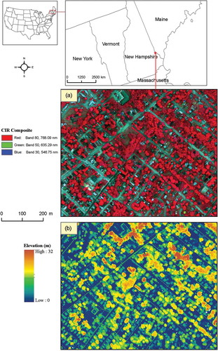
The study site is located in the City of Rochester (New Hampshire, USA) where NASA collected G-LiHT hyperspectral and LiDAR data on 8 June 2016. It covers an area of about 120 ac with five major land-cover types to be defined in this study, including buildings, trees, impervious ground (roads, parking lots, driveways, etc.), grass/lawn, and water/pools. Applying coarse-scale land-cover classification systems such as the standard scheme from Anderson et al. (1976) in urban areas is problematic because they cannot characterize the heterogeneity of urban environments. Selection of classes in this study was based on a modified fine-scale classification system developed by Cadenasso, Picket, and Schwarz (2007), which can account for the heterogeneity of human-built and natural components. So far, there is no standard for the fine-scale urban land-cover classification. The definition of classes depends on the study area, aim of the project, and the resolution of the input data (Lu and Weng 2007).

In this study, two G-LiHT data products were evaluated, including the 1-m at-sensor reflectance hyperspectral data and LiDAR-CHM products. G-LiHT acquires the 1-m hyperspectral imagery with 402 contiguous spectral bands (407–1007 nm) using a Hyperspec imaging spectrometer. G-LiHT collects both profiling and scanning LiDAR data. The scanning LiDAR data are collected by the VQ-480 airborne laser scanning instrument and the profiling LiDAR data are collected by an LD321-A40 multipurpose laser distance meter. The collected hyperspectral and LiDAR data are calibrated, processed, and distributed to the public as the standard data products at three levels by the G-LiHT team. Detailed data processing and product generation information can be found in Cook et al. (2013). In the G-LiHT dataset, original hyperspectral imagery (409 bands) is aggregated and resampled to the range of 418–919 nm, leading to a total of 114 bands for the at-sensor reflectance products. The 1-m LiDAR-CHM product is generated from the scanning LiDAR data. The LiDAR-CHM product is the same as the LiDAR normalized digital surface model (nDSM) used in the literature. The thermal product was not available for the study site and thus was not considered in this study. A color composite derived from the at-sensor reflectance product (bands 80, 50, and 30, as the red, green, and blue, respectively) and the LiDAR-CHM is shown in Figure 1 for the study site. Shadows are not problematic in the collected hyperspectral imagery because no high-rise developments and strong topographic features are present in the study site, and thus they are not considered.

Figure 1. The study site shown as (a) a color composite from the G-LiHT at-sensor reflectance product (bands 80, 50, and 30 as red, green, and blue, respectively) and (b) the LiDAR-CHM product (m, AGL).

To view this figure in color, please see the online version.

A total of 1032 image objects were selected as the reference data to calibrate and validate the techniques used in the evaluation. The image objects were produced by segmenting the 1-m at-sensor reflectance imagery, which are detailed in the next section. A spatially stratified data sampling strategy was followed in the reference object selection, in which a fixed percentage of samples were selected for each class. The number of reference objects was roughly estimated based upon the total number of generated image segments. The selected reference objects were manually labeled and refined by jointly checking the hyperspectral imagery, CHM, and a 2015 one-ft orthophoto. The selected reference objects for each class were split into two halves with one for calibration/training and the other for validation/testing. The number of training/testing samples for each class is listed in Table 3.

Table 1. Classification accuracies and statistical tests from different datasets and classifiers.

Experiments	OA (%)	Kappa	z-Score (Kappa)	z-Score (McNemar)
Hyperspectral data (114 bands)
1. k-NN	87.8	0.84	44.4	3.1^a, 2.5^a, 0.2, 1.7 (1/2, 1/3, 1/4, 1/7)
2. SVM	92.4	0.90	58.8	1.1, 1.0, 1.9 (2/3, 2/5, 2/8)
3. RF	90.9	0.88	51.1	0.2, 2.0^a (3/6, 3/9)
Multispectral data (4 bands)
4. k-NN	85.5	0.81	39.9	4.1^a, 3.9^a, 6.9^a (4/5, 4/6, 4/10)
5. SVM	91.1	0.88	53.5	0.0, 4.7^a (5/6, 5/10)
6. RF	91.1	0.88	53.5	4.3^a (6/10)
A fusion of hyperspectral data and LiDAR-CHM
7. k-NN	89.7	0.86	49.4	3.2^a, 2.3^a (7/8, 7/9)
8. SVM	94.4	0.93	69.2	1.1 (8/9)
9. RF	93.0	0.91	61.5	6.2^a, 3.3^a, 4.5^a, 5.6^a, 2.1^a, 3.9^a (1/10, 2/10, 3/10, 7/10, 8/10, 9/10)
10. EA	96.3	0.95	74.4

k-NN: k-nearest neighbor; SVM: support vector machine; RF: random forest; EA: ensemble analysis of k-NN, SVM, and RF; OA: overall accuracy. ^aSignificant with 95% confidence.

For the McNemar tests, 1/2, 1/3, 1/4, …, 9/10 refer to the test between Experiments 1 and 2, 1 and 3, 1 and 4, …, 9 and 10, respectively.

Table 2. Per-class accuracies from the fused dataset of G-LiHT hyperspectral data and LiDAR-CHM using three classifiers.

	User’s accuracy (%)			Producer’s accuracy (%)
Classes	k-NN	SVM	RF	k-NN	SVM	RF
1. Buildings	71.4	92.9	85.7	81.4	91.0	89.4
2. Trees	99.4	96.9	99.4	99.4	98.7	98.1
3. Impervious ground	88.5	92.0	92.0	75.2	91.2	83.2
4. Grass/Lawn	95.4	94.6	93.1	97.6	93.9	98.4
5. Water/Pools	68.8	93.8	81.3	100.0	100.0	100.0

The highest accuracy among three classifiers is in bold. k-NN: k-nearest neighbor; SVM: support vector machine; RF: random forest.

Table 3. Error matrix of the ensemble analysis using the fused dataset.

Class number	1	2	3	4	5	Row total	PA (%)
1	90		7	1		98	91.8
2		158		1		159	99.4
3	4		109			113	96.5
4		1	4	125		130	96.2
5			1		15	16	93.8
Col. total	94	159	121	127	15	Overall accuracy: 96.3%
UA (%)	95.7	99.4	90.1	98.4	100.0	Kappa value: 0.95

PA: Producer’s accuracy; UA: user’s accuracy.

Classification results are displayed in rows, and the reference data are displayed in columns. The name of each class is displayed in Table 2.

3. Methodology

3.1. A framework to combine G-LiHT hyperspectral and LiDAR-CHM products

The main objective of this study is to evaluate the ability of a fused dataset from G-LiHT hyperspectral and LiDAR-CHM products for urban/suburban land-cover mapping. In this context, the two data products should be combined first. Three strategies are commonly used to combine LiDAR and optical imagery for urban land-cover mapping: vector stacking, reclassification, and post-classification (Huang, Zhang, and Gong 2011; Priem and Canters 2016). Vector stacking extracts features from LiDAR and the imagery first and then combines them for use as classifier inputs to generate land-cover map. This is also known as feature-level fusion in multi-sensor data fusion applications (Gómez-Chova et al. 2015). Reclassification is the process by which spectral features extracted from imagery are classified first, and then imagery classification is integrated with LiDAR features to conduct a second classification. Post-classification also performs image classification first and then refines the outputs using LiDAR features by specifying rulesets. Evaluation of these three strategies showed that they could produce comparable classification accuracies (Huang, Zhang, and Gong 2011).

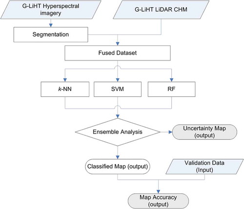
In all the above fusion strategies, only one classifier is adopted, and no attempts have been made to integrate the idea of ensemble analysis in the fusion procedure. In this study, an experimental framework was designed to integrate hyperspectral imagery and LiDAR data, as shown in Figure 2. In the framework, the fine spatial resolution hyperspectral imagery is segmented first to generate image objects and extract spectral/spatial features, and then the extracted features are combined with elevation features (statistical descriptors) derived from the LiDAR-CHM at the object level, leading to a fused dataset. This is similar to the first step of the vector stacking or feature-level fusion methods. Three machine-learning algorithms (k-NN, SVM, and RF) are used to pre-classify the fused dataset. The final outcome is derived through ensemble analysis of the three classifications using a decision-level fusion strategy. Note that the decision-level fusion strategy is based on the classification results of the fused dataset, rather than making a decision from the classification results of the individual data sources. The latter is commonly referred to as decision-level fusion in multi-sensor fusion applications. Consequently, an object-based land-cover map is generated and evaluated by common accuracy assessment approaches. The ensemble analysis of three classification results also produces an uncertainty map which defines the confidence of the classification for each image object. This has never been reported before in urban land-cover classification. Both feature-level and decision-level fusions are combined in the framework to integrate hyperspectral and LiDAR data for urban land-cover mapping. The developed fusion approach is thus referred to as the feature/decision-level fusion to be different from the commonly used fusion strategies. The major steps in the framework are detailed in the following subsections.

Figure 2. The framework to combine G-LiHT hyperspectral and LiDAR-CHM products for mapping urban land-cover types.

3.2. Image segmentation

To conduct object-based image classification, image objects must be produced first. The multiresolution segmentation algorithm in eCognition Developer 9.0 (Trimble 2014) was applied to generate image objects from the G-LiHT hyperspectral data. The segmentation algorithm requires the inputs of several parameters, including scale, color/shape, and smoothness/compactness. Efforts have been made to develop approaches for an optimal scale parameter in the segmentation (e.g., Grybas, Melendy, and Congalton 2017). In this study, an unsupervised image segmentation evaluation approach (Johnson and Xie 2011) was used to determine an optimal scale parameter. This approach begins with a series of segmentations using different scale parameters and then identifies the optimal image segmentation using a method that takes into account global intra-segment and intersegment heterogeneity measures. The evaluation revealed that a scale of 25 was optimal for this image. All 114 spectral bands of the image were set to equal weights, and color/shape weights were set to 0.5/0.5. Smoothness/Compactness weights were also set to 0.5/0.5 so as to not favor either compact or non-compact segments. Following segmentation, the spectral/spatial features of the hyperspectral imagery (mean and standard deviation) and LiDAR-CHM statistical descriptors (maximum, minimum, mean, and standard deviation) were extracted and merged at the object level as the input for the classification.

3.3. k-NN, SVM, and RF

In the experimental framework, three nonparametric machine-learning classifiers, k-NN, SVM, and RF classifiers, were employed to pre-classify the fused dataset. These classifiers have proven powerful to process hyperspectral data and fused datasets of multiple data sources and produced accurate mapping results in wetland environments (e.g., Zhang 2014; Zhang, Selch, and Cooper 2016) and coral reef ecosystems (Zhang 2015). k-NN identifies objects based on the closest training samples in the feature space. It searches away in all directions until it encounters k user-specified training objects and then assigns the object to the class with the majority vote of the encountered objects. k-NN needs to set the type of distance measures and the choice of k value. A recent review of this technique in remote sensing was conducted by Chirici et al. (2016). SVM is a supervised classifier with the aim to find a hyperplane that can separate the input dataset into a discrete predefined number of classes in a fashion consistent with the training samples (Vapnik 1995). Detailed descriptions of SVM algorithms were given by Huang, Davis, and Townshend (2002) in the context of remote sensing. Researchers commonly use the kernel-based SVM algorithms in the classification, among which the radial basis function and polynomial kernels are the most applied kernel functions. Both kernels were tested in this study. A detailed review of SVM in remote sensing was provided by Mountrakis, Im, and Ogole (2011). RF is a decision tree-based ensemble classifier. Detailed descriptions of RF can be found in Breiman (2001) and a recent review of RF in remote sensing was given in Belgiu and Drăguţ (2016). Two parameters need to be defined in RF: the number of decision trees to create and the number of randomly selected variables considered for splitting each node in a tree.

3.4. Ensemble analysis

The innovation of the designed framework is the combination of ensemble analysis in the mapping procedure. An ensemble analysis approach is a multiple classification system that combines the outputs of several classifiers. The classifiers in the system should generally produce accurate results but show some differences in classification accuracy (Du et al. 2012). A range of strategies has been developed to combine the outputs from multiple classifiers. Among these strategies, the majority vote strategy in which each individual classifier votes for an unknown input object is straightforward. A key problem of the majority vote is that all the classifiers have equal rights to vote without considering their performances on each individual class. A weighting strategy may mitigate this problem by weighting the decision from each classifier based on their accuracies obtained from the reference data. In this study, the majority vote and the weighting strategies are combined to analyze the outputs from the three classifiers. This combining strategy has proven useful to integrate the outputs of three classifiers (Zhang 2014; 2015; Zhang, Selch, and Cooper 2016). If three votes are different for an unknown object (e.g., k-NN votes class 1, SVM votes class 2, and RF votes class 3), then the unknown object will be assigned to the class which has the highest accuracy among the classifiers (i.e., class 2 because SVM has a higher accuracy than k-NN and RF in identifying class 1 and class 3, respectively). That is, the classifier with the best performance among three votes will obtain a weight of 1, while weights of the other two classifiers will be set at 0. If two or three classifiers vote the same class for an input object, then the object will be assigned to the same voted class. An uncertainty map can also be derived from the ensemble analysis of three classifiers. If three classifiers vote the same class for an unknown image object, a complete agreement will be achieved. Conversely, if three votes are completely different, no agreement will be obtained. If two classifiers vote for the same class, a partial agreement will be produced. Consequently, the uncertainty map will be produced in conjunction with the final classified map from the ensemble analysis.

3.5. Accuracy assessment

We applied the error matrix and Kappa statistics (Congalton and Green 2009) techniques to assess the accuracy of the classification. These methods have served as the standards in remote sensing image classification. The error matrix is summarized as an overall accuracy (OA) and Kappa value. The OA is defined as the ratio of the number of validation samples that are classified correctly to the total number of validation samples irrespective of the class. The Kappa value describes the proportion of correctly classified validation samples after random agreement is removed. McNemar test (Foody 2004) was adopted to evaluate the statistical significance of differences in accuracy between different classifications. The difference in accuracy of a pair of classifications is viewed as being statistically significant at a confidence of 95% if z-score is larger than 1.96.

4. Results

4.1. G-LiHT hyperspectral data product

We evaluated whether the G-LiHT hyperspectral product is more effective in mapping land cover compared with the broadband multispectral data. Fine spatial resolution satellite imagery such as Quickbird and Ikonos has proven successful in urban land-cover mapping (Myint et al. 2011). This type of imagery commonly has four broad spectral bands (red, green, blue, and near-infrared). Broadband multispectral data can be convolved from the hyperspectral data based on the sensor-specific spectral filter functions in ENVI version 4.7 (Exelis Visual Information Solutions, Boulder, Colorado). In this study, Quickbird data were simulated from the G-LiHT hyperspectral scene from the spectral resample function in ENVI, and the spatial/spectral value of each image object was calculated from the simulated Quickbird data in order to compare the performance of hyperspectral and multispectral sensors in urban land-cover mapping. The simulated Quickbird dataset and G-LiHT dataset represent the exact same location, geometry, spatial resolution, and boundary of each image object. Note that a real Quickbird image was not used because varying image objects might be produced from the Quickbird and G-LiHT data, which made the comparison challenging at the object level.

A total of six experiments were designed to assess the performance of G-LiHT hyperspectral sensor and Quickbird multispectral sensor. Experiments 1–3 applied three classifiers to the G-LiHT hyperspectral data. In contrast, experiments 4–6 classified the simulated Quickbird data (Table 1). Each model was implemented and tuned in WEKA, a machine-learning software package (Hall et al. 2009). The best results in terms of the OA achieved for the testing data are listed in Table 1. For the hyperspectral data, the SVM produced the best result among three classifiers with an OA of 92.4% and Kappa value of 0.90, while k-NN generated the lowest accuracy with an OA of 87.8% and Kappa value of 0.84. For the multispectral data, SVM and RF produced the same accuracy with an OA of 91.1% and Kappa value of 0.88. Again, k-NN generated the lowest accuracy among them with an OA of 85.5% and Kappa value of 0.81. Based upon the McNemar tests, the classifications results of the two datasets from SVM and RF were significantly different from the k-NN results, but there was no significant difference between SVM and RF in the classification. The McNemar tests also demonstrated that there was no statistically significant difference between the applications of two datasets in urban land-cover mapping when the same classifier was applied. Kappa statistical tests showed that all the classifications from experiments 1 to 6 were statistically better than a random classification.

4.2. A combination of G-LiHT hyperspectral and LiDAR-CHM data products

The G-LiHT hyperspectral and LiDAR-CHM products were combined using the feature-level fusion method to generate a fused dataset. The classification accuracies of the fused dataset from three classifiers are also listed in Table 1 as experiments 7–9. Again, the SVM produced the best result with an OA of 94.4% and Kappa value of 0.93, while k-NN had the lowest accuracy with an OA of 89.7% and Kappa value of 0.86. Classifications from SVM and RF showed a statistically significant difference from the k-NN classification. No significant difference was found between SVM and RF in the classification. In general, the accuracy was marginally increased compared with the application of the hyperspectral data alone (experiments 1–3). To examine whether such increase was statistically significant, McNemar tests were conducted again. The results demonstrated that there were no significant differences between the classifications of using hyperspectral data alone and the fused data when k-NN and SVM were used, but application of RF produced a significant difference between two datasets.

The per-class accuracies from experiments 7 to 9 are listed in Table 2. Performances of the three classifiers were not complete even in identifying each class. For example, from the user’s perspective, k-NN produced the best result in classifying class 4 (grass/lawn); SVM had the best performance in discriminating classes 1 (buildings) and 5 (water/pools). From the producer’s perspective, k-NN was the best in discriminating class 2 (trees); SVM was the best in identifying classes 1 and 3 (impervious ground); and RF produced the highest accuracy for class 4. This diversity is primarily caused by the discrepancies of three algorithms: k-NN searches for the best match to denote inputs; RF looks for optimal decision trees to group data, whereas SVM explores for the optimal hyperplane to categorize data. The diversity drives the exploration of the ensemble analysis which requires the difference in outputs from multiple classifiers. The ensemble analysis result is displayed as experiment 10 in Table 1. It increased the classification accuracy with an OA of 96.3% and Kappa value of 0.95. Similarly, McNemar tests were conducted between the classifications of experiment 10 and experiments 1–9. The results showed that the ensemble analysis significantly increased the classification effectiveness compared with the usage of each classifier alone. Inclusion of LiDAR-CHM product in the mapping procedure significantly increased the classification accuracy when the ensemble analysis was applied.

4.3. Land-cover and classification uncertainty mapping from ensemble analysis

The classified maps from three classifiers as well as the ensemble analysis using the combined dataset of G-LiHT hyperspectral and LiDAR-CHM products are shown in Figure 3(a–d). For comparison purposes, the segmentation of a portion of the study site is also displayed in Figure 3(e). In general, four dominant features (buildings, trees, impervious ground, and grass/lawns) were well depicted and small water ponds/pools were also identified by all the classifications. The experiments have shown that the ensemble analysis was the best classification, thus the error matrix of the ensemble analysis was calculated, as listed in Table 3. The user’s accuracies varied from 90.1% (impervious ground) to 100% (water), and the producer’s accuracies ranged from 91.8% (buildings) to 99.4% (trees). Note that the accuracies displayed in Table 3 might not be the “true accuracy” of the generated map. A non-exhaustive classification was conducted in this study, i.e., only the five dominant classes were specified in the training and mapping procedure. Minor surface features such as cars and shadows were excluded. The non-exhaustive training inevitably brings errors into the classified map because an object representing an area of an untrained class must be allocated, erroneously, to one of specified classes. Inclusion/Exclusion of the minor features in the training stage is a trade-off in the mapping procedure. For urban land-cover mapping, city mangers/planners are more concerned about the spatial distribution of the major land covers; minor features may be excluded from the training stage deliberately if they are not of interest. In addition, the exclusion of minor features in the training stage has the potential to reduce any spectral confusion between any minor and major features to be identified (Foody 2002).

Figure 3. The classified land-cover maps from the fused dataset using (a) k-NN, (b) SVM, (c) RF, and (d) ensemble analysis of three classifications; (e) the segmentation of a portion of the study site; and (f) the uncertainty map generated from ensemble analysis of three classifications.

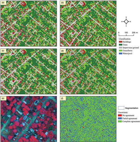
To view this figure in color, please see the online version.

The corresponding uncertainty map derived from the ensemble analysis is displayed in Figure 3(f). It was difficult to visually identify the difference between the classified maps (Figure 3a–d). The uncertainty map effectively revealed their consistency and difference. A major portion showed a complete agreement from three classifiers (shown in green), indicating the highest confidence being correctly classified. Some areas (shown in blue) were voted by two classifiers, generating a partial agreement in the classification. A few regions displayed a “warning sign” (shown in red), where no classification agreement was obtained. These regions had the highest probability of being misclassified. The uncertainty map demonstrated the classified maps were robust.

5. Discussion

5.1. Hyperspectral versus multispectral sensor for urban land-cover mapping

Literature has shown that for urban land-cover mapping, spatial resolution is more important than spectral resolution (Myint et al. 2011). Similar classifications were produced from the G-LiHT hyperspectral data product and the multispectral Quickbird data using the same classifier, indicating that high spectral resolution is unnecessary for broad land-cover mapping. A further analysis of the per-class classification showed that hyperspectral data improved the classification of impervious ground compared with the multispectral data (results were not shown). The impervious ground class includes roads, driveways, and parking lots in the study site, and it has the highest degree of within-class spectral variation among the five classes. The study indicated that hyperspectral data are more powerful in discriminating classes with a high within-class spectral diversity. For discriminating urban surface materials, however, the narrowband hyperspectral data have shown to be more effective than the broadband multispectral data (Herold et al. 2006). Note that the configuration of the G-LiHT hyperspectral sensor is different from NASA’s other hyperspectral sensor, the Airborne Visible/Infrared Imaging Spectrometer (AVIRIS), which collects data in the range of 380–2500 nm. Studies have shown that data over the shortwave infrared (1000–3000 nm) of AVIRIS are important for identifying some urban surface materials (Herold et al. 2006), while G-LiHT does not collect data over this region. It is valuable to assess the capabilities and limitations of G-LiHT hyperspectral data in mapping urban surface materials, which is one of the major objectives for future work.

Hyperspectral data have a high dimensionality. To effectively process a large volume of hyperspectral data, researchers commonly use a feature selection approach to reduce the data dimensionality. Less attention has been paid to the impact of dimensionality reduction on the classification. In this study, the comparison between the application of the full hyperspectral dataset and the simulated multispectral dataset can also assess the impact of dimensionality reduction on urban land-cover classification. The results here confirmed the study from Demarchi et al. (2014), who indicated that the dimensionality reduction of hyperspectral data had minor impacts on urban land-cover mapping when machine-learning classifiers were used. This is different from the results in the application of hyperspectral data for wetland vegetation classification, in which a dimensionality reduction method, in contrast, significantly increased classification accuracy (Zhang and Xie 2012). Benediktsson, Palmason, and Sveinsson (2005) and Pullanagari et al. (2017) reported slightly increased classification accuracy from reduced datasets when hyperspectral imagery was applied in urban land-cover mapping. But they did not conduct the significance test to determine whether such improvement was significant or not by combining the feature selection/extraction approach in the mapping procedure.

The application of hyperspectral data reduction is a difficult concession in the urban land-cover classification. On the one hand, inclusion of data reduction in the mapping procedure can reduce the computational burdens if a broad area needs to be mapped from hyperspectral data, but on the other hand, some spectral information might be lost after data reduction, leading to a lower accuracy, especially in mapping urban surface materials (Herold et al. 2006). In addition, a number of hyperspectral data reduction methods have been developed, which makes the selection of an effective method a difficult task.

When the fine spatial resolution imagery is applied in urban land-cover mapping, a range of spatial components, such as shape and texture features, can be extracted and combined with the spectral components to increase the classification effectiveness. Tong, Huan, and Weng (2014) systematically investigated the potential effects of these spatial components on urban land-cover mapping. It is, again, a trade-off in applying these spatial features. First, inclusion of these spatial features will result in a higher dimensionality of dataset, making the classification more complex. Second, an effective dimensionality reduction method needs to be identified so that informative features can be used. Failure of data dimensionality reduction might decrease the accuracy. Lastly, the effectiveness of these spatial components is scale dependent, and selecting an optimal scale for each spatial feature is a challenge. In this study, only the spectral mean and standard deviation were used in the classification. It is beyond the scope of this study to evaluate the contribution of each specific spatial feature derived from the G-LiHT hyperspectral data products in the classification.

5.2. Fusion of G-LiHT products for mapping urban land-cover types

Past studies have shown that LiDAR can significantly improve urban land-cover mapping compared with simply using optical imagery alone. For example, Huang, Zhang, and Gong (2011) found that inclusion of LiDAR elevation data was able to increase accuracy by 12% in classifying five land-cover classes compared with using a multispectral image alone (from 82.5% to 95.0%); Man, Dong, and Guo (2015) reported an accuracy increase of 6.8% when LiDAR-nDSM was combined with the hyperspectral data (from 81.7% to 88.5%). In this study, it was found that the improvement from LiDAR-CHM product was marginal (~2%) if just individual classifiers were applied. It is difficult to compare the results derived in this study with findings reported in other studies even though they were also conducted for urban land-cover mapping. Several factors might impact the results when LiDAR is combined with optical imagery for urban land-cover classification, including the fusion strategy, the classifier, the LiDAR features extracted from CHM/nDSM, the detail level to be mapped, and the complexity of study site. It was expected that LiDAR could improve the discrimination of classes with similar spectral features, but different elevations (e.g., grass and trees, impervious ground and buildings); however, LiDAR might add elevation confusion to grass/impervious ground and trees/buildings because they can have similar elevation statistics. Thus, inclusion of the G-LiHT LiDAR metrics product (LiDAR height, density, fractional cover and statistics, and etc.) might be more useful. This metrics product was not available when this study was conducted, but it was listed in the G-LiHT metadata and would be available soon. Another potential improvement might be achieved by using the original LiDAR point cloud statistics, rather than the raster LiDAR-CHM data. Working directly from the point cloud can produce a higher accuracy by preserving the original LiDAR values (Zhang 2014). We also examined G-LiHT LiDAR-intensity product (results were not shown) and found that it had no contribution in the classification. This was expected because the LiDAR intensity was collected from the near-infrared, which was already covered by the hyperspectral data.

5.3. Ensemble analysis in land-cover mapping

One major contribution of this study is the application of ensemble analysis of the outputs from three machine-learning classifiers. The SVM and RF produced a comparable result, and their classifications were statistically significant and better than the k-NN classification in processing both the fused dataset and the single-source hyperspectral data; however, the performance of the three classifiers in discriminating each individual class was not even. This drove us to combine the ensemble analysis technique in the framework. Ensemble analysis indeed increased the classification accuracy compared with the application of a single classifier in the classification, and the improvement was statistically significant. Another interesting finding was that when the ensemble analysis was applied to the fused dataset, the contribution from the LiDAR-CHM product became statistically significant; in contrast, application of a single classifier did not show classification improvement from the LiDAR-CHM. Ensemble analysis played an important role in the mapping procedure. Ensemble analysis can also contribute the classification uncertainty in the mapping procedure. It is able to produce an uncertainty map which can identify the geographic regions with a robust classification and areas where classification errors are most likely to occur. The traditional accuracy assessment approaches only provide the general quality of the classification without the capability of providing any geographic classification errors. The uncertainty map from the ensemble analysis is useful when there is a desire to minimize the omission or commission errors. It also can be used to guide the post-classification fieldworks (Foody, Boyd, and Sanchez-Hernandez 2007).

5.4. Limitation of the proposed framework

Although the developed framework achieved an encouraging result to combine G-LiHT hyperspectral and LiDAR products for mapping urban land-cover types, it suffers some limitations. First, the framework applied the full G-LiHT hyperspectral dataset without applying any feature selection/extraction approaches to reduce the high dimensionality. Note that applying such types of data for broad area mapping might be compute-intensive and the inclusion of LiDAR features will make the computation more intensive. Thus, for broad area mapping, feature selection/extraction should be explored and an appropriate data reduction method should be identified and applied. Second, there are limitations in applying OBIA for urban land-cover mapping, as discussed by Liu and Xia (2010) in detail. One major issue of OBIA is the specification of parameters for the segmentation, especially the scale parameter. Methods have been developed for the optimization of the scale parameter, including visual analysis, automated supervised, and unsupervised approaches (e.g., Drăguţ, Tiede, and Levick 2010; Johnson and Xie 2011; Johnson et al. 2015; Xun and Wang 2015; Su 2017). However, the single-scale segmentation approach might lead to errors from both over-segmentation and under-segmentation which would impact the final classification, even though an optimal scale parameter has been identified and applied for one scene. To mitigate this problem, a multi-scale segmentation approach was developed (Johnson and Xie 2011), but application of this approach to refine the over-segmented and under-segmented objects is complex. Thus, the single-scale segmentation approach is applied in the framework, which produces errors from both over-segmentation and under-segmentation. Other segmentation parameters such as color/shape are still specified empirically and subjectively. The last limitation is from the application of machine-learning classifiers in the framework. Machine-learning techniques are powerful for land-cover mapping, but they are data-driven approaches which require many training data to generate ideal results. In addition, these classifiers are also sensitive to the specification of the input parameters. Selecting optimal parameters for the SVM classifier is difficult (Lin and Yan 2016). Similarly, the ensemble analysis depends on what combining scheme will be used to integrate the outputs of different classifiers. The selection of an approach as well as the parameter specification for each approach will bring uncertainties in the final mapping result.

6. Summary and conclusions

A recent G-LiHT mission over an urban area provides a good opportunity to evaluate the fusion of G-LiHT hyperspectral and LiDAR data products for urban land-cover mapping. Two G-LiHT data products, at-sensor reflectance hyperspectral data and LiDAR-CHM, were assessed over a portion of the City of Rochester, New Hampshire. An experimental framework was designed to combine these two products. Contemporary remote sensing data processing techniques were integrated, including OBIA, machine-learning classifiers, and ensemble analysis. Major findings from this study are listed below:

1. The G-LiHT at-sensor reflectance hyperspectral product is able to classify five dominant land-cover types with the highest accuracy (92.4%) achieved by the SVM classifier. The 1-m G-LiHT hyperspectral product is powerful for urban land-cover mapping.

2. Fine spatial resolution multispectral imagery (e.g., Quickbird data) is adequate for mapping broad urban land-cover types and acquisition of hyperspectral data for such purpose is not necessary. The hyperspectral data did not show significant difference from the aggregated multispectral data in the classification. Comparable results were obtained from the hyperspectral and multispectral datasets for the study site.

3. The LiDAR-CHM product is useful to improve the classification. An inclusion of the LiDAR-CHM data in the framework marginally increased the classification effectiveness compared with the application of hyperspectral data alone. The highest accuracy was 94.4% from the SVM classifier.

4. Three machine-learning classifiers (k-NN, SVM, and RF) are effective in processing both the single-source hyperspectral data and fused hyperspectral and LiDAR data. All of these performed well in the classification. SVM and RF had a comparable performance, and both were better than the k-NN classifier.

5. Ensemble analysis is beneficial in the framework. It not only significantly increased the classification effectiveness, but it also provided an important uncertainty map which complemented the traditional accuracy assessment approaches. The idea of ensemble analysis can be extended into other data fusion strategies (e.g., reclassification and post-classification), as well as other land-cover classification applications.

6. The designed framework can be modified to integrate other data sources for land-cover classifications. Inclusion of the G-LiHT LiDAR metrics, thermal data, and vegetation indices products in the framework may further improve the urban land-cover mapping. Similarly, combining more advanced classifiers such as neural networks may be helpful as well. In addition, considerable work is needed to investigate its robustness and extensionality for more complex urban regions as well as other land-cover mapping applications. These will be major objectives in future research. It is anticipated that this study can stimulate the worldwide applications of G-LiHT products in general and the urban environments in particular.

Acknowledgments

Chaoyang Fang acknowledges the support from the National Science and Technology Program of China (2015BAH50F03), and the Collaborative Innovation Center for Major Ecological Security Issues of Jiangxi Province and Monitoring Implementation (No.JXS-EW-00).

Disclosure statement

No potential conflict of interest was reported by the authors.

References

- Akbari, D., S. Homayouni, A. Safari, and N. Mehrshad. 2016. “Mapping Urban Land Cover Based on Spatial-Spectral Classification of Hyperspectral Remote-Sensing Data.” International Journal of Remote Sensing 37: 2440–2445. doi:10.1080/01431161.2015.1129561.
- Anderson, J. R., E. E. Hardy, J. T. Roach, and R. E. Witmer. 1976. Land Use and Land Cover Classification Systems for Use with Remote Sensor Data. Washington, DC: US Geological Service. Professional Paper 964.
- Belgiu, M., and L. Drăguţ. 2016. “Random Forest in Remote Sensing: A Review of Applications and Future Directions.” ISPRS Journal of Photogrammetry and Remote Sensing 114: 24–31. doi:10.1016/j.isprsjprs.2016.01.011.
- Benediktsson, J. A., J. A. Palmason, and J. R. Sveinsson. 2005. “Classification of Hyperspectral Data from Urban Areas Based on Extended Morphological Profiles.” IEEE Transactions on Geoscience and Remote Sensing 43: 480–491. doi:10.1109/TGRS.2004.842478.
- Breiman, L. 2001. “Random Forests.” Machine Learning 45: 5–32. doi:10.1023/A:1010933404324.
- Cadenasso, M. L., S. T. A. Picket, and K. Schwarz. 2007. “Spatial Heterogeneity in Urban Ecosystems: Reconceptualizing Land Cover and a Framework for Classification.” Frontiers in Ecology and the Environment 5: 80–88. doi:10.1890/1540-9295(2007)5[80:SHIUER]2.0.CO;2.
- Chen, Z., and B. Gao. 2014. “An Object-Based Method for Urban Land Cover Classification Using Airborne Lidar Data.” IEEE Journal of Selected Topics in Applied Earth Observations and Remote Sensing 7: 4243–4254. doi:10.1109/JSTARS.2014.2332337.
- Chirici, G., M. Mura, D. McInerney, N. Py, E. O. Tomppo, L. T. Waser, D. Travaglini, and R. E. McRoberts. 2016. “A Meta-Analysis and Review of the Literature on the k-Nearest Neighbors Technique for Forestry Applications that Use Remotely Sensed Data.” Remote Sensing of Environment 176: 282–294. doi:10.1016/j.rse.2016.02.001.
- Chu, H.-J., C.-K. Wang, S.-J. Kong, and K.-C. Chen. 2016. “Integration of Full-Waveform LiDAR and Hyperspectral Data to Enhance Tea and Areca Classification.” GIScience & Remote Sensing 53: 542–559. doi:10.1080/15481603.2016.1177249.
- Congalton, R., and K. Green. 2009. Assessing the Accuracy of Remotely Sensed Data: Principles and Practices. 2nd ed. Boca Raton, FL: CRC/Taylor & Francis.
- Cook, B. D., L. W. Corp, R. F. Nelson, E. M. Middleton, D. C. Morton, J. T. McCorkel, J. G. Masek, K. J. Ranson, V. Ly, and P. M. Montesano. 2013. “NASA Goddard’s Lidar, Hyperspectral and Thermal (G-LiHT) Airborne Imager.” Remote Sensing 5: 4045–4066. doi:10.3390/rs5084045.
- Demarchi, L., F. Canters, C. Cariou, G. Licciardi, and C-W. Chan. 2014. “Assessing the Performance of Two Unsupervised Dimensionality Reduction Techniques on Hyperspectral APEX Data for High Resolution Urban Land-Cover Mapping.” ISPRS Journal of Photogrammetry and Remote Sensing 87: 166–179. doi:10.1016/j.isprsjprs.2013.10.012.
- Drăguţ, L., D. Tiede, and S. R. Levick. 2010. “ESP: A Tool to Estimate Scale Parameter for Multiresolution Image Segmentation of Remotely Sensed Data.” International Journal of Geographical Information Science 24: 859–871. doi:10.1080/13658810903174803.
- Du, P., J. Xia, W. Zhang, K. Tan, Y. Liu, and S. Liu. 2012. “Multiple Classifier System for Remote Sensing Image Classification: A Review.” Sensors 12: 4764–4792. doi:10.3390/s120404764.
- Foody, G. M. 2002. “Hard and Soft Classifications by a Neural Network with a Non-Exhaustively Defined Set of Classes.” International Journal of Remote Sensing 23: 3853–3864. doi:10.1080/01431160110109570.
- Foody, G. M. 2004. “Thematic Map Comparison, Evaluating the Statistical Significance of Differences in Classification Accuracy.” Photogrammetric Engineering & Remote Sensing 70: 627–633. doi:10.14358/PERS.70.5.627.
- Foody, G. M., D. S. Boyd, and C. Sanchez-Hernandez. 2007. “Mapping a Specific Class with an Ensemble of Classifiers.” International Journal of Remote Sensing 28: 1733–1746. doi:10.1080/01431160600962566.
- Forzieri, G., L. Tanteri, G. Moser, and F. Catani. 2013. “Mapping Natural and Urban Environments Using Airborne Multi-Sensor ADS40-MIVIS-LiDAR Synergies.” International Journal of Applied Earth Observation and Geoinformation 23: 313–323. doi:10.1016/j.jag.2012.10.004.
- Gerke, M., and J. Xiao. 2014. “Fusion of Airborne Laser Scanning Point Clouds and Images for Supervised and Unsupervised Scene Classification.” ISPRS Journal of Photogrammetry and Remote Sensing 87: 78–92. doi:10.1016/j.isprsjprs.2013.10.011.
- Ghamisi, P., J. A. Benediktsson, and S. Phinn. 2015. “Land-Cover Classification Using Both Hyperspectral and LiDAR Data.” International Journal of Image Data Fusion 6: 189–215. doi:10.1080/19479832.2015.1055833.
- Gómez-Chova, L., D. Tuia, G. Moser, and G. Camps-Valls. 2015. “Multimodal Classification of Remote Sensing Images: A Review and Future Directions.” Proceedings IEEE 103: 1560–1584. doi:10.1109/JPROC.2015.2449668.
- Grybas, H., L. Melendy, and R. G. Congalton. 2017. “A Comparison of Unsupervised Segmentation Parameter Optimization Approaches Using Moderate- and High-Resolution Imagery.” GIScience & Remote Sensing 54: 515–533. doi:10.1080/15481603.2017.1287238.
- Guan, H., J. Li, M. Chapman, F. Deng, Z. Ji, and X. Yang. 2013. “Integration of Orthoimagery and LiDAR Data for Object-Based Urban Thematic Mapping Using Random Forests.” International Journal of Remote Sensing 34: 5166–5186. doi:10.1080/01431161.2013.788261.
- Hall, M., E. Frank, G. Holmes, B. Pfahringer, P. Reutemann, and I. H. Witten. 2009. “The WEKA Data Mining Software: An Update.” SIGKDD Explorations 11: 10–18. doi:10.1145/1656274.1656278.
- Hamedianfar, A., H. Z. M. Shafri, S. Mansor, and N. Ahmad. 2014. “Combining Data Mining Algorithm and Object-Based Image Analysis for Detailed Urban Mapping of Hyperspectral Images.” Journal of Applied Remote Sensing 8: 085091. doi:10.1117/1.JRS.8.085091.
- Hardin, P., and A. Hardin. 2013. “Hyperspectral Remote Sensing of Urban Areas.” Geography Compass 7: 7–21. doi:10.1111/gec3.12017.
- Herold, M., S. Schiefer, P. Hostert, and D. A. Roberts. 2006. “Applying Imaging Spectrometry in Urban Areas.” In Urban Remote Sensing, edited by D. A. Quattrochi and Q. Weng, 137–162. Boca Raton, FL: CRC Press.
- Huang, C., L. S. Davis, and J. R. G. Townshend. 2002. “An Assessment of Support Vector Machines For Land Cover Classification.” International Journal of Remote Sensing 23: 725–749.
- Huang, X., L. Zhang, and W. Gong. 2011. “Information Fusion of Aerial Images and LiDAR Data in Urban Areas: Vector-Stacking, Re-Classification and Post-Processing Approaches.” International Journal of Remote Sensing 32: 69–84. doi:10.1080/01431160903439882.
- Johnson, B., M. Bragais, I. Endo, D. B. Magcale-Macandog, and P. B. M. Macandog. 2015. “Image Segmentation Parameter Optimization considering Within- and Between-Segment Heterogeneity at Multiple Scale Levels: Test Case for Mapping Residential Areas Using Landsat Imagery.” ISPRS International Journal of Geo-Information 4: 2292–2305. doi:10.3390/ijgi4042292.
- Johnson, B., and Z. Xie. 2011. “Unsupervised Image Segmentation Evaluation and Refinement Using a Multi-Scale Approach.” ISPRS Journal of Photogrammetry and Remote Sensing 66: 473–483. doi:10.1016/j.isprsjprs.2011.02.006.
- Khodadadzadeh, M., S. Member, J. Li, S. Prasad, and S. Member. 2015. “Fusion of Hyperspectral and LiDAR Remote Sensing Data Using Multiple Feature Learning.” IEEE Journal of Selected Topics in Applied Earth Observations and Remote Sensing 8: 2971–5983. doi:10.1109/JSTARS.2015.2432037.
- Kim, Y. 2016. “Generation of Land Cover Maps through the Fusion of Aerial Images and Airborne LiDAR Data in Urban Areas.” Remote Sensing 8: 521. doi:10.3390/rs8060521.
- Lin, Z., and L. Yan. 2016. “A Support Vector Machine Classifier Based on A New Kernel Function Model for Hyperspectral Data.” GIScience & Remote Sensing 53: 85–101. doi:10.1080/15481603.2015.1114199.
- Liu, D., and F. Xia. 2010. “Assessing Object-based Classification: Advantages and Limitations.” Remote Sensing Letters 1: 187–194.
- Lu, D., and Q. Weng. 2007. “A Survey of Image Classification Methods and Techniques for Improving Classification Performance.” International Journal of Remote Sensing 28: 823–870. doi:10.1080/01431160600746456.
- Luo, S., C. Wang, X. Xi, H. Zeng, D. Li, S. Xia, and P. Wang. 2016. “Fusion of Airborne Discrete-Return LiDAR and Hyperspectral Data for Land Cover Classification.” Remote Sensing 8: 0003. doi:10.3390/rs8010003.
- Man, Q., P. Dong, and H. Guo. 2015. “Pixel- and Feature-Level Fusion of Hyperspectral and LiDAR Data for Urban Land-Use Classification.” International Journal of Remote Sensing 36: 1618–1644. doi:10.1080/01431161.2015.1015657.
- Mountrakis, G., J. Im, and C. Ogole. 2011. “Support Vector Machines in Remote Sensing: A Review.” ISPRS Journal of Photogrammetry and Remote Sensing 66: 247–259. doi:10.1016/j.isprsjprs.2010.11.001.
- Myint, S. W., P. Gober, A. Brazel, S. Grossman-Clarke, and Q. Weng. 2011. “Per-Pixel vs. Object-Based Classification of Urban Land Cover Extraction Using High Spatial Resolution Imagery.” Remote Sensing of Environment 115: 1145–1161. doi:10.1016/j.rse.2010.12.017.
- Priem, F., and F. Canters. 2016. “Synergistic Use of LiDAR and APEX Hyperspectral Data for High-Resolution Urban Land Cover Mapping.” Remote Sensing 8: 787. doi:10.3390/rs8100787.
- Pullanagari, R., G. Kereszturi, I. J. Yule, and P. Ghamisi. 2017. “Assessing the Performance of Multiple Spectral-Spatial Features of a Hyperspectral Image for Classification of Urban Land Cover Classes Using Support Vector Machines and Artificial Neural Network.” Journal of Applied Remote Sensing 11: 026009. doi:10.1117/1.JRS.11.026009.
- Su, T. 2017. “Efficient Paddy Field Mapping Using Landsat-8 Imagery and Object-Based Image Analysis Based on Advanced Fractel Net Evolution Approach.” GIScience & Remote Sensing 54: 354–380. doi:10.1080/15481603.2016.1273438.
- Tong, X., X. Huan, and Q. Weng. 2014. “Urban Land Cover Classification with Airborne Hyperspectral Data: What Features to Use?” IEEE Journal of Selected Topics in Applied Earth Observations and Remote Sensing 7: 3998–4009. doi:10.1109/JSTARS.2013.2272212.
- Torbick, N., and M. Corbiere. 2015. “Mapping Urban Sprawl and Impervious Surfaces in the Northeast United States for the past Four Decades.” GIScience & Remote Sensing 52: 746–764. doi:10.1080/15481603.2015.1076561.
- Trimble. 2014. eCognition Developer 9.0.1 Reference Book. München: Definiens AG.
- Vapnik, V. N. 1995. The Nature of Statistical Learning Theory. New York: Springer-Verlag.
- Xun, L., and L. Wang. 2015. “An Object-Based SVM Method Incorporating Optimal Segmentation Scale Estimation Using Bhattacharyya Distance for Mapping Salt Cedar (Tamarisk Spp.). With QuickBird Imagery.” GIScience & Remote Sensing 52: 257–273. doi:10.1080/15481603.2015.1026049.
- Yan, W. Y., A. Shaker, and N. El-Ashmawy. 2015. “Urban Land Cover Classification Using Airborne LiDAR Data: A Review.” Remote Sensing of Environment 158: 295–310. doi:10.1016/j.rse.2014.11.001.
- Yang, H., B. Ma, Q. Du, and C. Yang. 2010. “Improving Urban Land Use and Land Cover Classification from High-Spatial-Resolution Hyperspectral Imagery Using Contextual Information.” Journal of Applied Remote Sensing 4: 041890. doi:10.1117/1.3491192.
- Zhang, C. 2014. “Combining Hyperspectral and LiDAR Data for Vegetation Mapping in the Florida Everglades.” Photogrammetric Engineering & Remote Sensing 80: 733–743. doi:10.14358/PERS.80.8.733.
- Zhang, C. 2015. “Applying Data Fusion Techniques for Benthic Habitat Mapping and Monitoring in a Coral Reef Ecosystem.” ISPRS Journal of Photogrammetry and Remote Sensing 104: 213–223. doi:10.1016/j.isprsjprs.2014.06.005.
- Zhang, C. 2016. “Multiscale Quantification of Urban Composition from EO-1/Hyperion Data Using Object-Based Spectral Unmixing.” International Journal of Applied Earth Observation and Geoinformation 47: 153–162. doi:10.1016/j.jag.2016.01.002.
- Zhang, C., D. Selch, and H. Cooper. 2016. “A Framework to Combine Three Remotely Sensed Data Sources for Vegetation Mapping in the Central Florida Everglades.” Wetlands 36: 201–213. doi:10.1007/s13157-015-0730-7.
- Zhang, C., and Z. Xie. 2012. “Combining Object-Based Texture Measures with a Neural Network for Vegetation Mapping in the Everglades from Hyperspectral Imagery.” Remote Sensing of Environment 124: 310–320. doi:10.1016/j.rse.2012.05.015.
- Zhang, J., X. Lin, and X. Ning. 2013. “SVM-based Classification of Segmented Airborne LiDAR Point Clouds in Urban Areas.” Remote Sensing 5: 3749–3775. doi:10.3390/rs5083749.
- Zhou, W. 2013. “An Object-Based Approach for Urban Land Cover Classification: Integrating Lidar Height and Intensity Data.” IEEE Geoscience and Remote Sensing Letters 10: 928–931. doi:10.1109/LGRS.2013.2251453.