Monitoring African water bodies from twice-daily MODIS observation

Abstract

Building on the availability of high revisit frequency Earth Observation satellites at medium spatial resolution (250 m), this study investigates the feasibility of temporal monitoring of water bodies at a continental scale with MODIS. A 2004–2010 time series of twice-daily observations covering the whole African continent was systematically processed using a surface water detection method to derive 10-day indicators describing the location, the intra- and inter-annual variability as well as the temporal characterization of water bodies (i.e. seasonal or permanent water and maximum extent). The multispectral surface reflectance transformation in the HSV color space allows a per-pixel identification of surface water. The water aggregation time indicator provides the water occurrence for each 10-day period built from the seven years of observations. The cartographic products were successfully cross-validated with already existing maps and water products. The validation of the water body maximum extent map estimates the commission error at less than 6% and the seasonality information was also found to be consistent with the Köppen climatic classification.

Keywords:

• water body
• temporal series
• remote sensing
• medium resolution
• global

1. Introduction

Given population growt4h and uneven distribution of water supply, better knowledge of the spatial distribution and temporal variability of inland surface water resources is critically needed in view of sustainable development policies and management (Vörösmarty et al. 2000). The Global Climate Observing System (GCOS) includes as Essential Climate Variables (ECV) lake areas and water levels (GCOS 2011). These two variables are needed to support the climate studies and the models required by the United Nations Framework Convention on Climate Change (UNFCCC). The “lake areas” ECV needs mapping of lakes and large reservoirs which directly interfere with the local climate through evaporation and albedo (GCOS 2011). Moreover, flood and drought monitoring having dramatic economic and human impacts (Alsdorf and Lettenmaier 2003) need to be monitored in a more systematic way. Other application domains include human and animal health, food security – agriculture, cattle breeding, aquaculture, gardening – and biodiversity protection (UNESCO 2009; Vörösmarty et al. 2000). Up-to-date and timely information about surface water can be provided by two different but complementary approaches: mapping and monitoring.

First, the state of the art of surface water mapping at continental and global scales is reviewed. Although topographic mapping based on photogrammetry is a major source of information about inland water location, it is not consistent across countries and quickly becomes out-of-date due to its a long production cycle. Water body maps are thus often obtained from processing remotely sensed data whereas monitoring methods are implemented to generate timely information throughout the year. Water maps can be derived from various Earth Observation (EO) data such as optical imagery, SAR interferometry, LiDAR, and gravitational variation. Unfortunately, only optical imagery provides the measurements needed to monitor surface water with a sufficient revisit frequency yet (Alsdorf and Lettenmaier 2003; Musa, Popescu, and Mynett 2015; Wu and Liu 2015). In the past 15 years, various methods and datasets have been proposed to map surface water at the global or continental scale. Few global recent data set products are available with a spatial resolution equal to or higher than 1 km. Among these, three products were available when this study was conducted.

First, the widely used Global Lakes and Wetlands Database (GLWD) (Lehner and Döll 2004) is a compilation of many existing databases. However, according to Haas, Bartholomé, and Combal (2009), the use of this database as a standard reference is limited due to the quality and the production date of the source data.

Second, the Shuttle Radar Topography Mission Water Body Dataset (SWBD) (Slater et al. 2006) has a high spatial resolution (30 m). However, it describes the situation as observed at a specific acquisition time (February 2000). The acquisition conditions were not ideal for water bodies as they correspond to the dry season in Northern hemisphere semi-arid regions such as the Sahel. This is a season with low level and even drying out of many seasonal water bodies.

Third, the MODIS 250-m land-water mask (MOD44W) (Carroll et al. 2009) available on the Global Land Cover Facility is a one-off mapping product based on the combination of SRTM and MODIS data. Although the spatial resolution is 250 m, the dataset is not adequate for applications such as seasonal variability analysis.

After completion of this study, several global products with improved resolution became available. These include SAR-WBI (Santoro and Wegmuller 2014), the datamask from the Global Forest Change (Hansen et al. 2013), the ESA CCI global map of open water bodies (Lamarche et al. 2017), the Global Inland Water (GIW) v1.0 (Feng et al. 2016) and the Global 3 arc-second Water Body Map (G3WBM) (Yamazaki, Trigg, and Ikeshima 2015). Other products were announced in the literature but are not available such as the Global Water Bodies database (GLOWABO) (Verpoorter et al. 2014) and the Global Water Pack (Klein et al. 2015). Lamarche et al. (2017) compare these products in terms of spatial extent, completeness, thematic accuracy, inland water/ocean discrimination and spatial resolution. Although these products provide major improvements in global inland surface water characterization, none of them propose an annual map update or dynamic monitoring.

In addition to inland surface water mapping, several studies have been published on their monitoring. In addition to ad hoc mapping for crisis management (Kugler and De Groeve 2007), it was shown that surface variation of smaller temporary reservoirs in semi-arid regions due to changing seasonal rainfall patterns can be monitored with optical EO data (Gond et al. 2004; Gardelle et al. 2010; Haas et al. 2011). Other methods have demonstrated the potential to monitor water surface at continental or global scale from satellite remote sensing. Mueller et al. (2016) proposed and applied a water detection algorithm to map the presence of surface water across Australia on 27 years of satellite imagery. Khandelwal et al. (2017) tested a MODIS-based algorithm to map surface water bodies at 500 m with eight-day intervals and demonstrated it for five reservoirs on four continents. Nevertheless, there are only two operational continental water body monitoring systems. First, the NASA wetland Earth Science Data Record (ESDR) (NASA-JPL 2014) delivering a global 10-day flood map at the resolution of 25 km, which is too coarse to measure most of the natural fluctuations. Second, an operational system monitoring small water bodies, first for the Sahelian zone and then scaled up to Africa, uses 10-day syntheses of SPOT-VGT data (Bartholomé 2008). Based on a contextual algorithm (Gond et al. 2004), the product was developed and validated for sub-humid and semi-arid regions where it performs well (Haas 2010). Due to limitations observed over dense vegetation areas, it cannot be successfully used at a continental scale. To expand the monitoring at a continental scale, another method was proposed. First developed for locust monitoring (Pekel et al. 2014), then adapted to water (Pekel et al. 2014), a method using a colorimetric transformation was used to monitor water bodies over time and derive indicators (d’Andrimont et al. 2010; d’Andrimont, Pekel, and Defourny 2011). More recently, the detection method proposed by Pekel et al. (2014) was successfully adapted to Landsat and applied on a 32-year archive by Pekel et al. (2016).

Building on the availability of high revisit frequency EO observations at medium spatial resolution, this work aims to map and monitor the seasonal variability of water bodies at continental scale. More specifically, the first objective is to assess the performance of the algorithm proposed by Pekel et al. (2014) to retrieve the water body extent at continental scale. The second objective is to propose and test indicators to characterize the inter-annual and intra-annual variabilities along with the water seasonality. This is done by using a 7-year time series of MODIS daily surface reflectance acquired over the African continent.

2. Data and study area

Four MODIS daily surface reflectance products (collection 5, L2G) are used: (i) Aqua Surface Reflectance at 250 m (MYD09GQ), (ii) Terra Surface Reflectance at 250 m (MOD09GQ), (iii) Aqua Surface Reflectance at 500 m (MYD09GA), and (iv) Terra Surface Reflectance at 500 m (MOD09GA). They were downloaded from the Land Processes Distributed Active Archive Center (LP DAAC) to cover the African continent over a 7-year period, from 2004 to 2010. The study area ranges from 30^° North to 40^° South and from 30^° West to 60^° East. Three wavelengths are considered: the Red and the Near-InfraRed (NIR) at 250 m and the Middle InfraRed (MIR) at 500 m.

In addition to the reflectance products, the MODIS Aqua 8-day Land Surface Temperature & Emissivity products (MYD11A2 collection 5) at 1-km spatial resolution were also downloaded from the LP DAAC to cover the entire African continent over a 4-year period, from 2005 to 2008. The MODIS Land Surface Temperature (LST) used in this study is derived from two thermal infrared channels, i.e. bands 31 (10.78–11.28 µm) and 32 (11.77–12.27 µm) using the split-window algorithm (Wan et al. 2002) which corrects for atmospheric effects and uses an emissivity look-up table based on global land surface emissivity in the thermal infrared (Snyder et al. 1998).

3. Methodology

3.1. Water detection

3.1.1 Data pre-processing

The three steps before water detection are the surface reflectance compositing, the composite color space transformation, and the LST average diurnal amplitude computation. These methods are chosen for their robustness and computation speed which together make them good candidates for operational applications requiring near real-time information delivery (Pekel et al. 2014).

First, the MODIS surface reflectance measured twice-daily by Aqua and Terra platforms is composited over a 10-day interval (1 to 10, 11 to 20 and 21 to the end of each month) using the Mean Compositing algorithm. This method averages the valid cloud free reflectance values from both Aqua and Terra, based on the standard data quality flags (Vancutsem, Bicheron et al. 2007; Vancutsem, Pekel et al. 2007). This compositing method, assuming that the remaining noise in the daily reflectance is mainly random or can be averaged out, was also selected in the framework of GLC2000 (Mayaux et al. 2004; Bartholomé and Belward 2005), GlobCover (Defourny et al. 2006; 2009), and other land-cover mapping initiatives (Gond et al. 2004; 2005). The resulting composites are projected from sinusoidal to Lat/long projection (WGS84 datum). The 500-m MIR channel is resampled to 250 m resolution using the nearest-neighbor resampling algorithm.

Second, the 10-day MIR, NIR, and Red reflectance bands are assigned to Red, Green, and Blue (RGB) colors respectively to be transformed into the Hue, Saturation, and Value (HSV) color space using a standardized colorimetric transformation (Smith 1978). Decoupling the chromaticity (H and S) and the brightness (V) is adapted for developing a color image processing methodology requiring color specification for target identification and extraction (Pekel et al. 2014). This step makes it possible to apply the water surface detection algorithm in the Hue-Value subspace.

Finally, LST night and day composited products are averaged separately over four years to derive the diurnal amplitude which is a proxy of the thermal inertia of land surfaces (Price 1977; Pekel et al. 2014).

3.1.2 Water detection methodology

The “H-V space” methodology is summarized here below and further described in Pekel et al. (2014). A large sampling of objects corresponding to several millions of pixels spread over time – different seasons and different years between 2004 and 2010 – and through space – from the desert to the dense humid forest – are collected. They are then used to characterize the open water surface signatures (including lakes, dams, rivers, temporary and permanent water bodies, with different depths, sediments and organic loads) and the “other land surfaces” (sands, rocks, lava flows, bright and salt soils, steppes, savannas, shrubs, dry forests, humid forests, swamp forests, rainfed, and irrigated croplands, cities). The colorimetric properties of these two categories are noticeably separated in the H-V space with limited risk of confusion in most cases (97% of observations). They can therefore be discriminated through a simple threshold.

An additional discrimination criterion is needed for the overlapping region between the two categories as observed in the H-V space (less than 3% of observations). These ambiguous pixels are exclusively located in dark lava flow areas in the desert. A dark lava flows mask, characterized by very large thermal amplitude during the diurnal cycle (up to 25^°C), is obtained and allows removal of the ambiguous pixels.

3.2. Temporal analysis

Water body dynamics may be summarized by different indicators according to the temporal scale of interest. After compositing the daily data into a 10-day synthesis which is then transformed to H-V space, the pixels are classified as land, water or no data if no valid cloud free reflectance is available during the 10-day period (Figure 1). In this study, a decade is referred to a 10-day period. The water detection time series are then used to provide indicators corresponding to different aspects of water dynamics depicting their inter-annual variability, their intra-annual variability and their temporal characterization, i.e. seasonal or permanent water and water body maximum extent.

Figure 1. For each pixel, a 7-year decadal water detection provides information about (a) inter-annual variability, (b) intra-annual variability, and (c) temporal characterization.

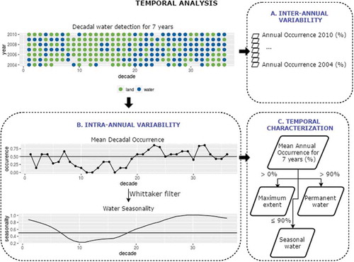
3.2.1. Inter-annual variability

In order to characterize inter-annual variation, the Annual Occurrence is defined as the percentage of time when water is detected for a given year (Figure 1(a)). The ratio Annual Occurrence (Equation (1)) is the division of the sum of the detected water states ($\omega$) by the sum of the valid observations (v) over the decades (d) for a given year (y) and for each pixel:

(1) $AnnualOccurrenc{e}_y=\frac{{\sum }_{d=0}^{d=36}{\omega }_d}{{\sum }_{d=0}^{d=36}{v}_d}.$(1)

The water state, defined as $\omega \in \left\{0,1\right\}$ corresponds respectively to non-water and water. The valid observation $v\in \left\{0,1\right\}$ equals 0 when no cloud free observation is available during the decade and 1 when at least one cloud free observation is available during the decade.

3.2.2. Intra-annual variability

In addition to inter-annual variability, a second indicator is Water Seasonality, representing the intra-annual variation of water state for each pixel. To obtain the seasonality, the water state for each 10-day period from 2004 to 2010 is used to calculate the Mean Decadal Occurrence which is then smoothed for each pixel and for each decade (d) through a two-step calculation (Figure 1(b)).

First, the Mean Decadal Occurrence for a given pixel and a given decade (d) is calculated by dividing the sum of the water states ($\omega$) detected by the sum of the valid observations (v) across years (y) (Equation (2)):

(2) $MeanDecadalOccurrenc{e}_d=\frac{{\sum }_{y=1}^{y=7}{\omega }_d}{{\sum }_{y=1}^{y=7}{v}_d}$(2)

Second, although reflectance data sets are pre-processed to reduce noise from sensor resolution and calibration, digital quantization errors, ground and atmospheric conditions, and orbital and sensor degradation, some noise is still present, including noise that results from cloud cover, poor atmospheric conditions, unfavorable sun-sensor-surface viewing geometries, detection failure and gaps in the time series (Pettorelli et al. 2005; Kobayashi and Dye 2005; Geng et al. 2014). Therefore, a temporal smoothing is applied the Mean Decadal Occurrence profile obtained with 7 years. Of the temporal profile smoothing techniques available in the literature, the Whittaker filter (Eilers 2003) was selected for its simple implementation and compatibility with massive processing. Moreover, the filter is flexible as it does not need any a priori assumption and it has a capacity to interpolate the missing values automatically. Eilers (2003) adapted the algorithm published in 1923 by Whittaker to a smoother able to fit discrete series. Geng et al. (2014) compared eight smoothers with MODIS data and concluded that the Whittaker smoother was the best temporal interpolator. As described by Atzberger and Eilers (2011), the aim is to fit a smooth series z to a noisy series y while balancing two conflicting goals: fidelity to the data and roughness of z. A balanced combination of the two goals is the sum Q (Equation (3)) which needs to be minimized to obtain the z smoothed series. The sum of squared differences S (Equation (4)) measures the fit to the data. R (Equation (5)) is the smoothed curve and corresponds to the second order differences. The smoothing parameter ($\lambda$) is chosen by the user. Increasing $\lambda$ value serves to increase the influence of R on Q at the cost of degradation of the fit:

(3) $Q=S+\lambda R,$(3)

with

(4) $S=\sum _i(y_i-z_i{)}^2,$(4)

(5) $R=\sum _i((z_i-z_{i-1})-(z_{i-1}-z_{i-2}){)}^2.$(5)

The Whittaker smoothing parameter $\lambda$ is set to 5 as it has been found the most relevant to handle missing data and obtain a good profile from any vegetation NDVI yearly profile (Verhegghen, Bontemps, and Defourny 2014). This has a similar shape and amplitude to water dynamic seasonality profile. The smoothed Water Seasonality is obtained by applying the Whittaker filter on the Mean Decadal Occurrence profile. The smoothing is operated on the yearly profile extended by half a year before and half a year after in order to take into account the full annual cycle that occurs in between years.

The output, referred as Water Seasonality, is a 36-band file where each band corresponds to a different 10-day period depicting the smoothed water occurrence of each pixel. It permits visualization of the temporal water body dynamic as a profile (Figure 1(b)). A similar characterization of the dynamic of binary-state land-cover classes has already been proposed for burned areas and for snow seasonality (Lamarche et al. 2013; Rousseau et al. 2015).

3.2.3. Temporal characterization

Then next step, after characterizing inter- and intra-annual variability, is to classify the water as seasonal or permanent and obtain its maximum extent. This was calculated from the 36-decade Mean Decadal Occurrence in order to obtain a single-band product summarizing the water state for each pixel for the 7 years. The Mean Annual Occurrence is defined as the mean of Mean Decadal Occurrence over valid observations (Equation (6)):

(6) $MeanAnnualOccurrence{}_{7years}=\frac{{\sum }_{d=0}^{d=36}MeanDecadalOccurrenc{e}_d}{{\sum }_{d=0}^{d=36}{v}_d}.$(6)

The result is a map providing occurrence percentage suitable for any end-user threshold. In this study, different maps may be obtained by thresholding the $MeanAnnualOccurrence{}_{7years}$: the maximum extent water body map (> 0%), the seasonal water body map ($\le 90\mathrm{\%}$), and the permanent water body map (> 90% of the year) (Figure 1(c)).

3.3. Quality assessment of the temporal analysis

To evaluate the different product’s accuracy and their spatial and temporal consistency, three approaches were considered. First, the maximum extent water body map is assessed through a random sampling biased toward water areas. Second, an exhaustive comparison between the 10-day products and existing products is carried out. Finally, the Water Seasonality is matched to climatic zone distribution to check possible macroscopic error in seasonality patterns.

3.3.1. Maximum extent water body map

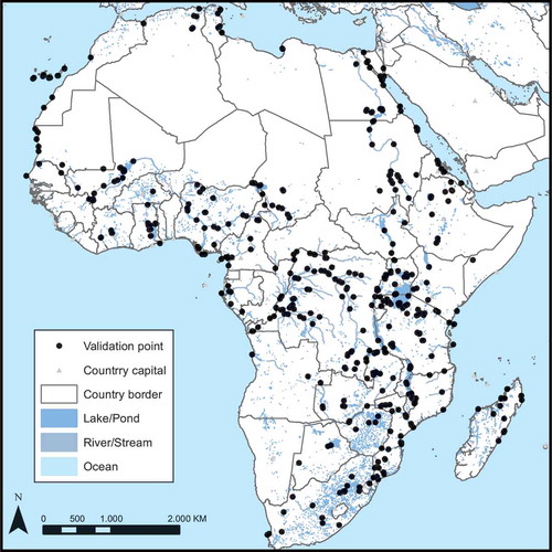
In order to assess the product commission error (i.e. false detection of water), a stratified random sampling is drawn to assess the maximum extent water body map over 7 years. As inland water surface corresponds to less than 3% of the African continent, and major lakes and coastlines make up the larger part of these detected water surfaces, the sampling is biased to over-sample the temporary water bodies and the rim of permanent water bodies that fluctuate over time. In order to over-sample changing water bodies, the inner part of major lakes is disregarded. To this end, the SWBD is used to create a 1-km inner buffer in the lake center direction for the 10 major African lakes. Moreover, a coastal mask derived from the GlobCover map (Defourny et al. 2006) is used to avoid selecting samples in the ocean.

A random sampling of 500 points in the water maximum extent excepting inner major lakes and ocean is then drawn (Figure 2). The MODIS pixel footprint corresponding to each sample is then displayed on Google Earth imagery to proceed with the photo-interpretation of high and very high resolution images. According to the photo-interpretation practices building on convergence of evidence (Estes and Simonett 1975; Teng et al. 1997), it is possible to identify water presence at the time of imaging, but also surfaces that may be seasonally flooded. Consequently, the “ground truth” database is no longer restricted to a single date snapshot. Each sample is labeled as “water”, “non-water,” or “undetermined.” A sample is considered as water when more than half of the pixel surface is covered by water or by a floodable surface. The pixel is undetermined if the visual interpretation is not reliable. This sampling strategy is designed to estimate the commission error of the algorithm but not the omission error as the no-water class is not sampled.

Figure 2. Distribution of 500 points randomly drawn in the potential water extent over Africa to assess the maximum extent water body map commission error.

3.3.2. Product comparisons

The product quality was also assessed by comparison with two other available water products. First, the permanent water body map was compared to the MOD44W product (Carroll et al. 2009). Second, the decadal detection output was compared with the Small Water Body product (SWB), which is valid over the Sahelian zone. The implementation of this SWB algorithm allowed monitoring of small water bodies and of the seasonality of temporary humid areas in an operational manner from January 1999 until 2014 using SPOT-VGT.¹ It should be noted that the SWB product confirms detection of a given decade only when the detection also took place for the same pixel during the previous decade. For the assessment, four decades are selected with a 3-month interval to capture the temporal variability over a year. The year 2010 is selected as it is considered as a normal year in West Africa.

To compare the products, discrepancy matrices are compiled along with the calculation of the Overall Quantity Disagreement (OQD) (Equations (7) and (8)) and the Overall Allocation Disagreement (OAD) (Equations (9) and (10)) as defined by Pontius and Millones (2011). In our notation, $p_{ij}$ is the estimated proportion of the study area that is in class i in the assessed map and in class j in the reference map. The number of categories is J for both:

(7) $QD=\left|\left(\sum _{i=1}^J{p}_{ij}\right)-\left(\sum _{j=1}^J{p}_{ji}\right)\right|,$(7)

(8) $OQD=\frac{{\sum }_{j=1}^{J}QD}{2},$(8)

(9) $AD=2min\left[\left(\sum _{i=1}^J{p}_{ij}\right)-p_{jj},\left(\sum _{j=1}^J{p}_{ji}\right)-p_{jj}\right],$(9)

(10) $OAD=\frac{{\sum }_{j=1}^{J}AD}{2}.$(10)

3.3.3. Linking water seasonality to climate classification

The Köppen-Geiger climate classification map (Kottek et al. 2006) is used to compute the distribution of permanent and seasonal water body areas per climatic zone. For this analysis, four water body seasonality classes are defined according to their persistence within the year (3 seasonal and 1 permanent): (a) less than 1/3 of the decades, (b) between 1/3 and 2/3 of the decades, (c) between 2/3 and 90% of the decades, and (d) more than 90% of the decades. The relative proportions of the different classes are then compared with the respective climatic zone.

4. Results

This very first continental scale experiment of surface water detection provides temporally and spatially consistent results. This demonstrates the potentiality of water body mapping at a decadal frequency, which could open interesting avenues for near real-time monitoring.

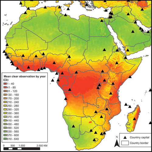
4.1. Valid data availability for water body detection

A major challenge is the persistent cloudiness over a part of Central and West Africa. Figure 3 represents the average number of valid cloud free observations throughout the year. In spite of the 2 MODIS observations a day provided by both Aqua and Terra satellites, the annual average number of cloud-free observations is lower than 20 observations a year along the Atlantic coast and is nil for the coastal zone of Nigeria (up to 70 km buffer over land). The continent may be divided into two parts identifying the type of possible applications for each zone: (1) regions with more than 150 cloud free observations a year are suitable for near real-time monitoring and inter-annual comparison as well as for water body mapping, and (2) regions with less than 150 observations a year (corresponding to about 1 observation out 5 of the potential observations) are not suited for near real-time monitoring with MODIS. For these cloudy regions, where water scarcity is usually not a major issue, data aggregation over multi-year time series still provides quite consistent results for permanent water body mapping.

Figure 3. Average number of valid observations over a year from both MODIS instruments calculated from 7 years (2004–2010).

4.2. Temporal analysis

4.2.1. Inter-annual variability

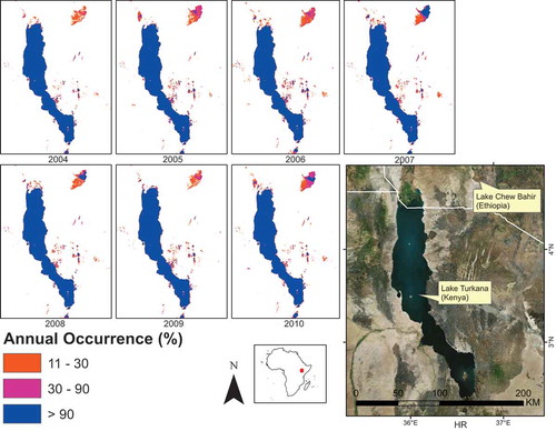
As a measurement of inter-annual fluctuation, the Annual Occurrence for each year from 2004 to 2010 was obtained and is illustrated over Lake Turkana and Lake Chew Bahir in Figure 4. This product monitors the extent of shrinking or expansion of water over several years. However, the results were less robust than the Mean Annual Occurrence as they were based on only one year and may therefore be limited in areas with important cloud coverage.

Figure 4. Annual Occurrence (%) from 2004 to 2010 on Lake Turkana (Kenya) and Lake Chew Bahir (Ethiopia) shows the inter-annual fluctuations of water extent. HR is a high resolution satellite imagery.

4.2.2. Intra-annual variability

Based on the decadal detections from 7 years, the Mean Decadal Occurrence was obtained and was then used to calculate Water Seasonality. Figure 5 illustrates seasonality over the Niger River in Mali for different types of water: seasonal (point 1 and 3) and permanent (point 2).

4.2.3. Temporal characterization

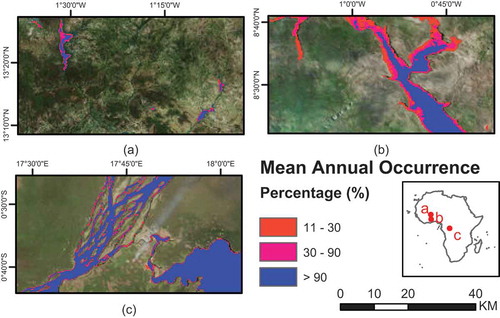
The Mean Annual Occurrence map depicts the water according to its mean frequency of observation through the year. Figure 6(a) shows small water bodies in the Sahelian zone where temporary water bodies were predominant. Figure 6(b) corresponds to a section of Lake Volta where dam management for power production and natural conditions induce a significant fluctuation in the water extent. Figure 6(c) shows the River Congo and a fraction of Lake Ntomba depicted clearly in the equatorial forest. Despite high cloud-cover frequency, time series aggregation provides a spatially consistent discrimination between water surface types according to their more or less seasonal nature.

Figure 5. Three pixel temporal profiles of River Niger in Mali (a) show the potential of the approach in obtaining seasonality profiles for seasonal, point 1 (16.22^° N, 3.65^° W) and 3 (16.22^° N, 3.89^° W) and permanent surface water, point 2 (16.27^° N, 3.69^° W). Intra-annual water variation is obtained from the decadal detections from 7 years providing the Mean Decadal Occurrence which is then smoothed to retrieve Water Seasonality.

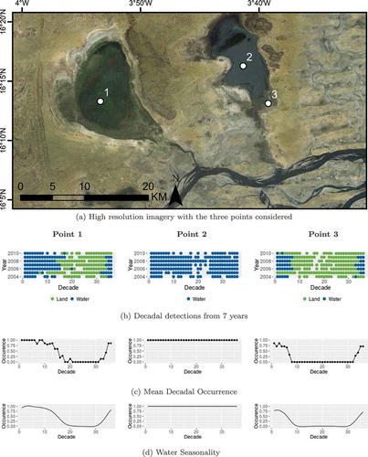
Figure 6. Mean Annual Occurrence (%) calculated from 7 years is displayed in three classes for three different extents: (a) large water body surface fluctuation in the Sahel, where temporary water bodies were predominant, (b) Lake Volta, where fluctuations are caused by anthropogenic and natural drivers, and (c) the River Congo, clearly shown in spite of significant cloud cover.

However, water extent fluctuation of one pixel can also be attributed to geometric accuracy or be caused by poor observational coverage (referred to as obscov). Indeed, in the case of MODIS, the instrument design and the way the information is stored in a grid can have strong impacts at pixel level (Tan et al. 2006).

Additionally, by thresholding the Mean Annual Occurrence, the maximum extent of water, together with seasonal and permanent water body maps for the 2004–2010 period has been retrieved, so providing valuable information for inventory purposes as well as input to model. The permanent water body map is shown in Figure 7.

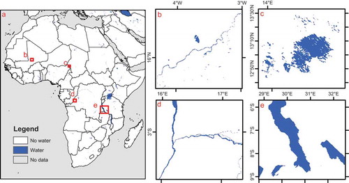
Figure 7. Overview of the 250-m permanent water body map (a) and subsets revealing the spatial consistency of the map in various contexts: the Niger river (b), Lake Chad (c), the River Congo, (d) and the Lake Tanganyika and Lake Rukwa (e).

4.3. Quality assessment of the temporal analysis

4.3.1. Maximum extent water body map

The commission error of the maximum extent water body map was evaluated by a systematic comparison of 500 points randomly distributed according to the sampling design previously described. The commission error obtained was 5.42% (Table 1).

Table 1. The commission error of the maximum extent water body map is evaluated by visual interpretation of 500 random samples using high and very high resolution images. Two samples were undetermined and thus removed from the assessment resulting in 498 points.

Output map
Reference	Water
Non-water	27 (5.42 %)
Water	471 (94.52 %)
Total	498 (100 %)

4.3.2. Product comparisons

The first comparison was completed between the permanent water body map and the MOD44W product. The discrepancy matrix presented in Table 2 shows a good overall agreement between products (99.78%), and specifically for the detected water (1.1%). The permanent water body map depicts more water (1.26%) than the static MOD44W product (1.16%) corresponding to more than 8% in relative difference. This was expected as the observation used for the latter corresponds only to the dry period for the whole of West and East Africa while the former is computed from a 7-year time series.

Table 2. Discrepancy matrix between the water body map and MOD44W (the results are given as percentages and do not include ocean and “no data” values).

MOD44W
Water body map	No water	Water	Total
No water	98.68	0.16	98.84
Water	0.06	1.10	1.16
Total	98.74	1.26	99.78

To further analyze these results, water body extent discrepancies larger than 50 km² were systematically assessed on high resolution imagery.

First, among the potential commission errors, i.e. detected as water by the permanent water body map and non-water by MOD44W, there were 47 polygons greater than 50 $k{m}^2$ among which only 19 were effectively commission errors (the remaining 28 were thus errors in MOD44W). The remaining 19 commission error areas were distributed in the following landscapes: dark rocks (12), salty lakes (2), volcanic rocks (4) and undefined (1). Distribution among the countries is Chad (9), Ethiopia (4), Libya (2), Eritrea (2), Algeria (1) and Western Sahara (1).

Second, among the potential omission errors, i.e. detected as non-water by the permanent water body map and water by MOD44W, there were 43 polygons greater than 50 km² among which only 14 were effectively omission errors (the 29 remaining were thus errors in MOD44W). The remaining 14 omission errors were lakes (6), desert lakes (3) chott and salt lakes (2), rivers (2) and sebkhas (1). The omission error distribution across countries is as follows: Egypt (5), Algeria (3), Chad (2), Niger (1), Nigeria (1), Tanzania (1) and Tunisia (1).

A second comparison highlights the discrepancies between the 10-day water product with SWB, a dynamic water body product available over Western Sahel. In order to compare the 250-m MODIS product with the 1-km SPOT-VGT SWB product, the MODIS products were aggregated to the SPOT-VGT grid using the mode algorithm. This was done for 4 decades distributed at 3-month intervals in the year 2010. As the SWB method is designed for semi-arid regions, both products were clipped on the semi-arid region. Afterwards, they were reclassified to obtain 2 classes (non-water and water): the humid vegetation class in the SWB was thus reclassified as non-water and no data from both products were removed.

Finally, the cross-tabulation matrices comparing the 4 selected decades are presented in Table 3 and shows that for the 4 decades, the MODIS-based product detects more water than the SWB products due to its finer spatial resolution. On the other hand, the relative seasonal variation computed for the 4 decades is consistently the same for both products. Table 3 provides information about disagreement between products. The overall quantity disagreements (OQD) are small (0.01–0.26) while the overall allocation disagreements (OAD) are slightly larger (0.56–0.73). However, the agreements between products are high (98.84–99.68%) and thus the quantity of disagreement is limited, the overall allocation disagreements showing that the disagreements result from the pixels location. In conclusion, the comparisons reveal that the amount of water of each class is close but that their pixels are not located at the same place.

Table 3. Comparison of water body monitoring by SPOT-VGT SWB and MODIS-based products for 4 decades of 2010 in Western Sahel.

SPOT-VGT SWB
Discrepancies (%)				Disagreement
	Non-water	Water	Sum	Allocation (OAD)	Quantity (OQD)
MODIS 1–10 January 2010				0.68	0.02
Non-water	99.19	0.01	99.20
Water	0.69	0.11	0.80
Sum	99.88	0.12	99.30
MODIS 1–10 April 2010				0.71	0.01
Non-water	99.54	0.03	99.57
Water	0.36	0.07	0.43
Sum	99.90	0.10	99.61
MODIS 1–10 July 2010				0.73	0.01
Non-water	99.64	0.04	99.68
Water	0.28	0.04	0.32
Sum	99.72	0.08	99.68
MODIS 1–10 October 2010				0.56	0.26
Non-water	98.64	0.04	98.68
Water	1.12	0.20	1.32
Sum	99.76	0.24	98.84

4.3.3. Linking water seasonality to climate classification

The seasonality of water bodies corresponds to what is expected for each climate type. This also demonstrates how quantitative water body dynamics could be measured and may be used as a quantitative ecosystem indicator. Table 4 reports the distribution of the different water body seasonality classes aggregated by climatic regions of the Köppen–Geiger climate classification (Kottek et al. 2006). The resulting distribution of the seasonality classes closely corresponds to what is expected from a climatic point of view. For the Equatorial zone, permanent water corresponds to the dominant climate type observed (from 81% for “fully humid” area to 61% for “winter dry” area). For the arid class (represented by “B”), the permanent water proportion is smaller than temporary water. Moreover, almost half of the observed water surfaces lasts for less than 4 months for the cold arid “BSk” (46%) and the cold arid desert “BWk” (43%) climatic regions. Both BSk and BWk are located in Northern Africa and Southern Africa. For the warm temperate climate (“C”), the area with a dry summer (“Csa”, “Csb”) and with a dry winter and a hot summer (“Cwa”) are characterized by equal proportions of the different seasonal classes: one third of temporary water bodies lasting less than 4 months, one third of temporary water bodies lasts for more than 4 months and one third are permanent water bodies.

Table 4. Water surface distribution percentage according to persistence within the year for each Köppen–Geiger climate class.

The Köppen–Geiger climate types are classified according to main climate (A: equatorial; B: arid; C: warm temperate), precipitation (W: desert; S: steppe; f: fully humid; s: summer dry; w: winter dry) and temperature (h: hot arid; k: cold arid; a: hot summer; b: warm summer; c: cool summer). Background gray bars represent the percentage for each seasonality class.

5. Discussion

In this section, the major limitations of the proposed approach along with proposed mitigation measures and potential improvements are discussed.

5.1. Optical input data

Despite the recent and forthcoming launches of the optical Sentinel satellites, especially Sentinel-2 and Sentinel-3 both of which are suited for water body monitoring, MODIS with its twice-daily revisit will remain a challenger in terms of frequency to imaging the globe. Indeed, neither Sentinel-2 nor Sentinel-3, will provide a better revisit frequency at global scale. Therefore, the limitations about cloud coverage will remain a limitation factor in the coming years as already highlighted by Whitcraft et al. (2015). High cloud coverage in some areas together with the presence of snow, reduce the available data and limit 10-day water detection. In areas where data is lacking for most 10-day syntheses, the algorithm is not able to ensure continuous near real-time detection. Frequent cloud coverage is likely to hinder reliable water body monitoring as well as inter-annual anomaly analysis in the equatorial zones, in spite of the twice-daily overpasses. For these equatorial zones, the synergistic use of SAR observation with optical should be investigated. In addition to the revisit frequency, the quality of cloud, shadow and snow screening is crucial for water body detection performance. Indeed, the presence of clouds leads to both omission and commission errors. On the one hand, the water detection algorithm tends to miss water when unscreened clouds are present; on the other hand, unscreened cloud shadows lead to false water detection. False detection also occurs over ice and snow areas, especially at the border of the permanent snows. Similarly, the heterogeneity of the observation conditions, such as sun and view angles, are influencing the measured reflectance. Therefore, specific methods handling heterogeneity over large area, such as proposed by d’Andrimont, Marlier, and Defourny (2017), may improve the water mapping.

Another limitation is that the reflectance obtained after atmospheric correction may be negative on water bodies as a result of aerosols load overestimation over very low water-leaving radiance (Li, Gong, and Shan 2009). Therefore a water body mask is used to apply specific atmospheric correction over water. Usually this water mask is not dynamic, so major artifacts may be observed such as “no data” over large lakes (Pekel et al. 2014) and limit detection performance. Using dynamic water masks for atmospheric correction could limit this caveat in the future.

A specific limitation of MODIS sensors comes from their whisk-broom imaging system resulting in a MODIS grid that does not correspond to the observation footprint. The particular design of the instrument and the way the information is stored in a grid have strong impacts (Tan et al. 2006). For that reason, MODIS reflectance is provided along with an observational coverage value (obscov), which defines the observation/grid cell intersection area divided by the area of the observation footprint (Wolfe, Roy, and Vermote 1998). It has been demonstrated that this obscov information could be taken into account in remote-sensing applications to limit its effects (Duveiller, Baret, and Defourny 2011). For water bodies with a size close to the pixel, the obscov could limit the effective resolution of the resulting product. The obscov information could be integrated into the compositing process to weight the reflectance and so mitigate this effect.

5.2. Validation

There is room for improvements of the validation approach especially for surface water monitoring.

First, the accuracy assessment sampling based on 500 points in water makes it possible to evaluate the commission error for the maximum extent water body map. During photo-interpretation of the sampling, a pixel footprint was labeled as water when at least half of its surface was covered or could be covered by water. This definition used for the assessments penalizes the product for pixel cover by 50 to 100% of water not detected by MODIS. Using a definition closer to the sensor detection potential such as, a pixel fully covered by water, could limit the overestimation of the commission error.

Second, comparison of the permanent water body map with MOD44W makes it possible to retrieve discrepancy matrices. Again, the definition of the water class is crucial and could be a limitation for validation. Here permanent is defined as having a Mean Annual Occurrence greater than 90%, while in MOD44W, there is no clear definition for permanent water.

Third, the comparisons of 10-day period maps with existing SWB products provide discrepancy matrices along with disagreement metrics. The comparison reveals a small overall quantity disagreement but a large overall allocation disagreement between products. Clearly, such an approach is limited as the sampling through time was limited to 4 dates in one year. A recent publication about validation of a dynamic burned area product from MODIS (Boschetti, Stehman, and Roy 2016) proposes a sampling design scheme based on a stratification with equal sample allocation among strata and integrates time as a variable for the sampling design. The study shows it is effective in reducing the standard errors of accuracy and area estimators. Such an approach could be envisaged to assess water body dynamic maps in the future.

Future assessments could take into account the contribution of the spatial resolution to the error. Boschetti, Flasse, and Brivio (2004) introduced the concept of the Pareto boundary to quantify and isolate the effect of the spatial resolution (mixed pixels) on the accuracy of a map. They illustrated how, for a given resolution, mixed pixels introduce a bias acting as a conflicting objective when trying to minimize the omission or the commission error. This approach has been successfully applied in several contexts such as cropland mapping (Waldner et al. 2016), Desert locust habitat monitoring (Waldner et al. 2015), and burned area mapping (Mallinis and Koutsias 2012).

5.3. Transferability of the detection method

While the detection method is well suited to water detection at continental scale and is transferable to other sensors, some limitations have been highlighted in this study.

The major limitation of the method is the need to adapt the thresholds according to the sensors used. After having tested the MODIS Hue-Value thresholds on SPOT-VGT and PROBA-V, it appears that the thresholds selected in the Hue-Value space do not provide the same results.

In addition, because of the equation used to obtain the Hue, slight differences in MIR, NIR and Red may induce major changes in Hue. As Hue values are different for water bodies when computed from the reflectances of two different sensors, the same thresholds cannot be used for making a consistent detection of water. This limitation implies that new thresholds should be defined to transfer the methodology to another sensor.

Future work could be focused on providing a statistical automated method for best thresholds selection along with the sampling used to set up thresholds. Alternatively, the use of expert systems has proved to be efficient in dealing with the range of conditions encountered (Pekel et al. 2016).

5.4. How to manage false detections?

After having tested the algorithm in various conditions with different sensors, some major false detections still remained but these were identified and removed. Indeed, the algorithm made false detections over some very low reflectance values such as topographical shadows, dark rocks and lava flows. As already mentioned, other areas wrongly detected were ice and snow areas, in particular at the edge of permanent snow. To mitigate these false detections, we propose a false-detection mask obtained in five steps which allows removal of the major systematic commission errors made by the algorithm.

The rationale was to mask areas where water was detected by the algorithm but was not present in external reference products and at the same time covered by glaciers, or located on steep slopes, or on high altitudes. This masking was confirmed through high-resolution imagery photo-interpretation. In practical terms, the maximum extent water body map was compared to a compilation of external global permanent water references in order to retrieve all the areas of potential commission errors. The second step then masks the permanent glaciers as mapped by the Randolph Glaciers Inventory (Pfeffer et al. 2014) and SCAR data (Fox et al. 2013). The third step masks the commission errors over steep slopes by using the SRTM CGIAR at 90-m (Jarvis et al. 2008) with the definition of Martinis et al. (2013):: the dynamic water bodies were unrealistic over areas of steep incline (>10^°), or significant height and lower slope (> 2000 m and a slope of >8^°). Finally the polygons of the mask were visually assessed on high resolution imagery (i.e. Google Earth and Bing). After visual analysis, the polygons identified as potentially covered by water were removed from the mask to avoid masking water. This last step was the major limitation as it requires time-consuming photo-interpretation. Applying such a mask makes it possible to reduce most of the systematic false detections.

6. Conclusions

Simple and robust image-processing methods were sufficient to retrieve reliable information about the location and, the intra- and inter-annual variability of water bodies in Africa from a 7-year MODIS dataset. Moreover, the method is sufficiently simple to be easily implemented in an operational processing chain to generate timely or near real-time water status information (where enough data is available) for water management and environmental monitoring purposes. This continent-wide experiment indicates that global scale mapping of water bodies and their seasonal dynamic could be achieved from multi-year time series. The output of this experiment also delivered a map of permanent inland open water surfaces, a map of their average seasonal status and an intra-annual seasonality profile from every location in Africa. The seasonal duration of water bodies as identified from the MODIS data is in agreement with the climatic regions defined by the Köppen–Geiger climatic classification. This underlines the interest for climate change studies of analyzing the behavior of small water bodies along with larger lakes and reservoirs.

Future research should focus on expanding this approach geographically to global scale and on improving the generic qualities of the method to make it transferable to other sensors. Nevertheless, all the presented limitations should be addressed. Another promising perspective it to adapt the proposed approach to higher resolution sensors such as Landsat and Sentinel-2. This could lead to better characterization of water surface dynamics, which are currently limited.

Acknowledgement

The authors thank the support from UCL and from Eric Van Bogaert and Thomas Demaet for the data processing. Moreover, the author would like to thank the reviewers for having improved the quality of the manuscript.

Disclosure statement

No potential conflict of interest was reported by the authors.

Additional information

Funding

This work was supported by the Geoland2 project, funded by European Commission within the 7th Framework Program.

Notes

1. The SWB product used in this study was downloaded from the Copernicus GIO Global land portal (http://land.copernicus.eu/global/products/wb) where it is referenced as WB V1.4.

References

- Alsdorf, D. E., and D. P. Lettenmaier. 2003. “Tracking Fresh Water from Space.” Science 301 (5639): 1491–1494. doi:10.1126/science.1089802.
- Atzberger, C., and P. H. C. Eilers. 2011. “Evaluating the Effectiveness of Smoothing Algorithms in the Absence of Ground Reference Measurements.” International Journal of Remote Sensing 32 (13): 3689–3709. doi:10.1080/01431161003762405.
- Bartholomé, E. 2008. “Monitoring the Environment in Africa: The VGT4Africa and the AMESD Projects.” In Proceedings of the 2nd International Workshop on “Crop and Rangeland Monitoring in East Africa”, Nairobi 27-29 March 2007.- Office for Official Publications of the European Commission, Luxembourg EUR 23546-2008, 303–319. European Commission.
- Bartholomé, E., and A. S. Belward. 2005. “GLC2000: A New Approach to Global Land Cover Mapping from Earth Observation Data.” International Journal of Remote Sensing 26 (9): 1959–1977. doi:10.1080/01431160412331291297.
- Boschetti, L., S. P. Flasse, and P. A. Brivio. 2004. “Analysis of the Conflict between Omission and Commission in Low Spatial Resolution Dichotomic Thematic Products: The Pareto Boundary.” Remote Sensing of Environment 91 (3): 280–292. doi:10.1016/j.rse.2004.02.015.
- Boschetti, L., S. V. Stehman, and D. P. Roy. 2016. “A Stratified Random Sampling Design in Space and Time for Regional to Global Scale Burned Area Product Validation.” Remote Sensing of Environment 186: 465–478. doi:10.1016/j.rse.2016.09.016.
- Carroll, M. L., J. R. Townshend, C. M. DiMiceli, P. Noojipady, and R. A. Sohlberg. 2009. “A New Global Raster Water Mask at 250 M Resolution.” International Journal of Digital Earth 2 (4): 291–308. doi:10.1080/17538940902951401.
- d’Andrimont, R., C. Marlier, and P. Defourny. 2017. “Hyperspatial and Multi-Source Water Body Mapping: A Framework to Handle Heterogeneities from Observations and Targets over Large Areas.” Remote Sensing 9 (3): 211. doi:10.3390/rs9030211.
- d’Andrimont, R., J.-F. Pekel, and P. Defourny. 2011. “Monitoring African Surface Water Dynamic Using Medium Resolution Daily Data Allows Anomalies Detection in Nearly Real Time.” 2011 6th International Workshop on The Analysis of Multi-Temporal Remote Sensing Images (Multi-Temp), 241–244, IEEE. Trento, July 12–14.
- d’Andrimont, R., J.-F. Pekel, E. Van Bogaert, and P. Defourny. 2010. “Monitoring Water Bodies over Whole Africa in near Real Time: Detection Algorithms and Preliminary Results.” Advances in Quantitative Remote Sensing (RAQRS) 3rd International Symposium. Torrent, September 27–October 01.
- Defourny, P., P. Bicheron, C. Brockman, S. Bontemps, E. Van Bogaert, C. Vancutsem, J.-F. Pekel, et al. 2009. “The First 300 M Global Land Cover Map for 2005 Using ENVISAT MERIS Time Series: A Product of the GlobCover System.” The 33rd International Symposium on Remote Sensing of Environment. Stresa, May 4–8.
- Defourny, P., C. Vancutsem, P. Bicheron, C. Brockmann, F. Nino, L. Schouten and M. Leroy. 2006. “GLOBCOVER: A 300 M Global Land Cover Product for 2005 Using Envisat MERIS Time Series.” In Proceedings of the ISPRS Commission VII Mid-Term Symposium, Remote Sensing: From Pixels to Processes, 8–11, Citeseer.Enschede, May 8–11.
- Duveiller, G., F. Baret, and P. Defourny. 2011. “Crop Specific Green Area Index Retrieval from MODIS Data at Regional Scale by Controlling Pixel-Target Adequacy.” Remote Sensing of Environment 115 (10): 2686–2701. doi:10.1016/j.rse.2011.05.026.
- Eilers, P. H. C. 2003. “A Perfect Smoother.” Analytical Chemistry 75 (14): 3631–3636. doi:10.1021/ac034173t.
- Estes, J. E., and D. S. Simonett. 1975. “Fundamentals of Image Interpretation.” Manual of Remote Sensing 1st ed. 869–1076.
- Feng, M., J. O. Sexton, S. Channan, and J. R. Townshend. 2016. “A Global, High-Resolution (30-M) Inland Water Body Dataset for 2000: First Results of a Topographic–Spectral Classification Algorithm.” International Journal of Digital Earth 9 (2): 113–133. doi:10.1080/17538947.2015.1026420.
- Fox, A., D. Herbert, P. Fretwell, and A. Fleming. 2013. SCAR Antarctic Digital Database V 6.0. http://nora.nerc.ac.uk/id/eprint/501478
- Gardelle, J., P. Hiernaux, L. Kergoat, and M. Grippa. 2010. “Less Rain, More Water in Ponds: A Remote Sensing Study of the Dynamics of Surface Waters from 1950 to Present in Pastoral Sahel (Gourma Region, Mali).” Hydrology and Earth System Sciences 14 (2): 309–324. doi:10.5194/hess-14-309-2010.
- GCOS. 2011. “Systematic Observation Requirements for Satellite-Based Products for Climate - 2011 Update - Supplemental Details to the Satellite-Based Component of the ‘Implementation Plan for the Global Observing System for Climate in Support of the UNFCCC (2010 Update)’.” Report. GCOS secretariat, WMO-Geneva. Access: http://cci.esa.int/sites/default/files/gcos-154.pdf
- Geng, L., M. Mingguo, X. Wang, Y. Wenping, S. Jia, and H. Wang. 2014. “Comparison of Eight Techniques for Reconstructing Multi-Satellite Sensor Time-Series NDVI Data Sets in the Heihe River Basin, China.” Remote Sensing 6 (3): 2024–2049. doi:10.3390/rs6032024.
- Gond, V., E. Bartholomé, F. Ouattara, A. Nonguierma, and L. Bado. 2004. “Surveillance et cartographie des plans d’eau et des zones humides et inondables en régions arides avec l’instrument VEGETATION embarqué sur SPOT-4.” [Monitoring and mapping of the wetlands and flood areas with the VEGETATION instrument on board of SPOT-4.] International Journal of Remote Sensing 25 (5): 987–1004. doi:10.1080/0143116031000139908.
- Gond, V., J. Bernard, C. Brognoli, 0. Brunaux, A. Coppel, J. Demenois, J. Engel, D. Galarraga, P. Gaucher, S. Guitet, F. Ingrassia, M. Lelievre, S. Linares, F. Lokonadinpoulle, R. Nasi, J-F. Pekel, D. Sabatier, V. Thierron, B. de Thoisy, J-F. Trebuchon, et G. Verger. 2009. Analyse multi-echelles de Ia caracterisation des ecosystemes forestiers guyanais et des impacts humains a partir de la teledetection spatiale [Multi-scale analysis of the characterization of Guyanese forest ecosystems and of the human impacts by remote sensing from space]. In Ecosystemes forestiers des caraibes, Karthala, 461–481.
- Haas, E. M. 2010. “Temporary water bodies as ecological indicators in West African drylands.” Thesis. Université Catholique de Louvain. http://hdl.handle.net/2078.1/32210 on 2016-12-01
- Haas, E. M., E. Bartholomé, E. F. Lambin, and V. Vanacker. 2011. “Remotely Sensed Surface Water Extent as an Indicator of Short-Term Changes in Ecohydrological Processes in sub-Saharan Western Africa.” Remote Sensing Of Environment 115: 3436–3445. doi:10.1016/j.rse.2011.08.007.
- Haas, E. M., E. Bartholomé, and B. Combal. 2009. “Time Series Analysis of Optical Remote Sensing Data for the Mapping of Temporary Surface Water Bodies in sub-Saharan Western Africa.” Journal of Hydrology 370 (1): 52–63. doi:10.1016/j.jhydrol.2009.02.052.
- Hansen, M. C., P. V. Potapov, R. Moore, M. Hancher, S. A. Turubanova, A. Tyukavina, D. Thau, et al. 2013. “High-Resolution Global Maps of 21st-Century Forest Cover Change.” Science 342 (6160): 850–853. doi:10.1126/science.1244693.
- Jarvis, A., H. I. Reuter, A. Nelson, and E. Guevara. 2008. “Hole-Filled SRTM for the Globe Version 4.” Available from the CGIARCSI SRTM 90m Database http://srtm.csi.cgiar.org.
- Khandelwal, A., A. Karpatne, M. Marlier, J. Kim, D. Lettenmaier, and V. Kumar. 2017. An Approach for Global Monitoring of Surface Water Extent Variations Using MODIS Data. Remote sensing of Environment.
- Klein, I., A. Dietz, U. Gessner, S. Dech, and C. Kuenzer. 2015. “Results of the Global WaterPack: A Novel Product to Assess Inland Water Body Dynamics on A Daily Basis.” Remote Sensing Letters 6 (1): 78–87. doi:10.1080/2150704X.2014.1002945#.VPbDQ3XN_CI.
- Kobayashi, H., and D. G. Dye. 2005. “Atmospheric Conditions for Monitoring the Long-Term Vegetation Dynamics in the Amazon Using Normalized Difference Vegetation Index.” Remote Sensing of Environment 97 (4): 519–525. doi:10.1016/j.rse.2005.06.007.
- Kottek, M., J. Grieser, C. Beck, B. Rudolf, and F. Rubel. 2006. “World Map of the Koppen-Geiger Climate Classification Updated.” Meteorologische Zeitschrift 15 (3): 259–263. doi:10.1127/0941-2948/2006/0130.
- Kugler, Z., and T. De Groeve. 2007. The Global Flood Detection System. Luxembourg: Office for Official Publications of the European Communities.
- Lamarche, C., S. Bontemps, A. Verhegghen, J. Radoux, E. Vanbogaert, V. Kalogirou, F. M. Seifert, O. Arino, and P. Defourny. 2013. “Characterizing The Surface Dynamics For Land Cover Mapping: Current Achievements Of The ESA CCI Land Cover.” In ESA Special Publication. Vol. 72279.
- Lamarche, C., M. Santoro, S. Bontemps, R. D’Andrimont, J. Radoux, L. Giustarini, C. Brockmann, J. Wevers, P. Defourny, and O. Arino. 2017. “Compilation and Validation of SAR and Optical Data Products for a Complete and Global Map of Inland/Ocean Water Tailored to the Climate Modeling Community.” Remote Sensing 9 (1): 36. doi:10.3390/rs9010036.
- Lehner, B., and P. Döll. 2004. “Development and Validation of a Global Database of Lakes, Reservoirs and Wetlands.” Journal of Hydrology 296 (1): 1–22. doi:10.1016/j.jhydrol.2004.03.028.
- Li, D., J. Gong, and J. Shan. 2009. Geospatial Technology for Earth Observation. Springer. doi:10.1007/978-1-4419-0050-0
- Mallinis, G., and N. Koutsias. 2012. “Comparing Ten Classification Methods for Burned Area Mapping in a Mediterranean Environment Using Landsat TM Satellite Data.” International Journal of Remote Sensing 33 (14): 4408–4433. doi:10.1080/01431161.2011.648284.
- Martinis, S., A. Twele, C. Strobl, J. Kersten, and E. Stein. 2013. “A Multi-Scale Flood Monitoring System Based on Fully Automatic MODIS and TerraSAR-X Processing Chains.” Remote Sensing 5 (11): 5598–5619. doi:10.3390/rs5115598.
- Mayaux, P., E. Bartholomé, S. Fritz, and A. Belward. 2004. “A New Land-Cover Map of Africa for the Year 2000.” Journal of Biogeography 31 (6): 861–877. doi:10.1111/jbi.2004.31.issue-6.
- Mueller, N., A. Lewis, D. Roberts, S. Ring, R. Melrose, J. Sixsmith, L. Lymburner, et al. 2016. “Water Observations from Space: Mapping Surface Water from 25years of Landsat Imagery across Australia.” Remote Sensing of Environment 174: 341–352. doi:10.1016/j.rse.2015.11.003.
- Musa, Z. N., I. Popescu, and A. Mynett. 2015. “A Review of Applications of Satellite SAR, Optical, Altimetry and DEM Data for Surface Water Modelling, Mapping and Parameter Estimation.” Hydrology and Earth System Sciences 19 (9): 3755–3769. doi:10.5194/hess-19-3755-2015.
- NASA-JPL. 2014. “Wetland Web-site. Global monitoring of wetland extend and dynamics.”, Accessed 2014. http://wetlands.jpl.nasa.gov/science/index.html
- Pekel, J.-F., Cottam, A., Gorelick, N., and Belward, A. S. 2016. “High-Resolution Mapping of Global Surface Water and Its Long-Term Changes.” Nature 540 (7633): 418–422. doi:10.1038/nature20584.
- Pekel, J.-F., C. Vancutsem, L. Bastin, M. Clerici, E. Vanbogaert, E. Bartholomé, and P. Defourny. 2014. “A near Real-Time Water Surface Detection Method Based on HSV Transformation of MODIS Multi-Spectral Time Series Data.” Remote Sensing of Environment 140: 704–716. doi:10.1016/j.rse.2013.10.008.
- Pettorelli, N., J. O. Vik, A. Mysterud, J.-M. Gaillard, C. J. Tucker, and N. C. Stenseth. 2005. “Using the Satellite-Derived NDVI to Assess Ecological Responses to Environmental Change.” Trends in Ecology & Evolution 20 (9): 503–510. doi:10.1016/j.tree.2005.05.011.
- Pfeffer, W. T., A. A. Arendt, A. Bliss, and T. Bolch. 2014. “The Randolph Glacier Inventory: A Globally Complete Inventory of Glaciers.” Journal of Glaciology 60 (221): 537–552. doi:10.3189/2014JoG13J176.
- Pontius, R. G., and M. Millones Jr. 2011. “Death to Kappa: Birth of Quantity Disagreement and Allocation Disagreement for Accuracy Assessment.” International Journal of Remote Sensing 32 (15): 4407–4429. doi:10.1080/01431161.2011.552923.
- Price, J. C. 1977. “Thermal Inertia Mapping: A New View of the Earth.” Journal of Geophysical Research 82 (18): 2582–2590. doi:10.1029/JC082i018p02582.
- Rousseau, C., Radoux, J., De Maet, T., Lamarche, C. and Defourny, P. 2015. “Snow Cover Anomalies from 2000 to 2014: Highlight of Two Exceptional Years over Europe.” In IGARSS 2015. Milano, July 13–18.
- Santoro, M., and U. Wegmuller. 2014. “Multi-Temporal Synthetic Aperture Radar Metrics Applied to Map Open Water Bodies.” IEEE Journal of Selected Topics in Applied Earth Observations and Remote Sensing 7 (8): 3225–3238. doi:10.1109/JSTARS.2013.2289301.
- Slater, J. A., G. Garvey, C. Johnston, J. Haase, B. Heady, G. Kroenung, and J. Little. 2006. “The SRTM Data “Finishing” Process and Products.” Photogrammetric Engineering & Remote Sensing 72 (3): 237–247. doi:10.14358/PERS.72.3.237.
- Smith, A. R. 1978. “Color Gamut Transform Pairs.” ACM Siggraph Computer Graphics 12 (3): 12–19. doi:10.1145/965139.807361.
- Snyder, W. C., Z. Wan, Y. Zhang, and Y. Z. Feng. 1998. “Classification-Based Emissivity for Land Surface Temperature Measurement from Space.” International Journal of Remote Sensing 19 (14): 2753–2774. doi:10.1080/014311698214497.
- Tan, B., C. E. Woodcock, J. Hu, P. Zhang, M. Ozdogan, D. Huang, W. Yang, Y. Knyazikhin, and R. B. Myneni. 2006. “The Impact of Gridding Artifacts on the Local Spatial Properties of MODIS Data: Implications for Validation, Compositing, and Band-To-Band Registration across Resolutions.” Remote Sensing of Environment 105 (2): 98–114. doi:10.1016/j.rse.2006.06.008.
- Teng, W. L., E. R. Loew, D. I. Ross, V. G. Zsilinszky, C. P. Lo, W. R. Philippson, W. D. Philpot, and S. A. Morain. 1997. “Fundamentals of Photographic Interpretation.” In American Society of Photogrammetry. 2nd ed. 49–116.
- UNESCO. 2009. “World Water Assessment Program 2009: The 3rd United Nations World Water Development Report: Water in a Changing World (WWDR-3).” Report. London: UNESCO. http://unesdoc.unesco.org/images/0018/001819/181993e.pdf
- Vancutsem, C., P. Bicheron, P. Cayrol, and P. Defourny. 2007a. “An Assessment of Three Candidate Compositing Methods for Global MERIS Time Series.” Canadian Journal of Remote Sensing 33 (6): 492–502. doi:10.5589/m07-056.
- Vancutsem, C., J. F. Pekel, P. Bogaert, and P. Defourny. 2007. “Mean Compositing, an Alternative Strategy for Producing Temporal Syntheses. Concepts and Performance Assessment for SPOT VEGETATION Time Series.” International Journal of Remote Sensing 28 (22): 5123–5141. doi:10.1080/01431160701253212.
- Verhegghen, A., S. Bontemps, and P. Defourny. 2014. “A Global NDVI and EVI Reference Data Set for Land-Surface Phenology Using 13 Years of Daily SPOT-VEGETATION Observations.” International Journal of Remote Sensing 35 (7): 2440–2471. doi:10.1080/01431161.2014.883105.
- Verpoorter, C., T. Kutser, D. A. Seekell, and L. J. Tranvik. 2014. “A Global Inventory of Lakes Based on High-Resolution Satellite Imagery.” Geophysical Research Letters 41 (18): 6396–6402. doi:10.1002/2014GL060641.
- Vörösmarty, C. J., P. Green, J. Salisbury, and R. B. Lammers. 2000. “Global Water Resources: Vulnerability from Climate Change and Population Growth.” Science 289 (5477): 284–288. doi:10.1126/science.289.5477.284.
- Waldner, F., D. De Abelleyra, S. R. Verón, M. Zhang, W. Bingfang, D. Plotnikov, S. Bartalev, et al. 2016. “Towards a Set of Agrosystem-Specific Cropland Mapping Methods to Address the Global Cropland Diversity.” International Journal of Remote Sensing 37 (14): 3196–3231. doi:10.1080/01431161.2016.1194545.
- Waldner, F., M. A. B. Ebbe, K. Cressman, and P. Defourny. 2015. “Operational Monitoring of the Desert Locust Habitat with Earth Observation: An Assessment.” ISPRS International Journal of Geo-Information 4 (4): 2379–2400. doi:10.3390/ijgi4042379.
- Wan, Z., Y. Zhang, Q. Zhang, and L. Zhao-Liang. 2002. “Validation of the Land-Surface Temperature Products Retrieved from Terra Moderate Resolution Imaging Spectroradiometer Data.” Remote Sensing of Environment 83 (1): 163–180. doi:10.1016/S0034-4257(02)00093-7.
- Whitcraft, A., I. Becker-Reshef, B. Killough, and C. Justice. 2015. “Meeting Earth Observation Requirements for Global Agricultural Monitoring: An Evaluation of the Revisit Capabilities of Current and Planned Moderate Resolution Optical Earth Observing Missions.” Remote Sensing 7 (2): 1482–1503. doi:10.3390/rs70201482.
- Wolfe, R. E., D. P. Roy, and E. Vermote. 1998. “MODIS Land Data Storage, Gridding, and Compositing Methodology: Level 2 Grid.” IEEE Transactions on Geoscience and Remote Sensing 36: 1324–1338. doi:10.1109/36.701082.
- Wu, G., and Y. Liu. 2015. “Combining Multispectral Imagery with in Situ Topographic Data Reveals Complex Water Level Variation in China’s Largest Freshwater Lake.” Remote Sensing 7 (10): 13466–13484. doi:10.3390/rs71013466.
- Yamazaki, D., M. A. Trigg, and D. Ikeshima. 2015. “Development of a Global 90m Water Body Map Using Multi-Temporal Landsat Images.” Remote Sensing of Environment 171: 337–351. doi:10.1016/j.rse.2015.10.014.