Landsat-8 vs. Sentinel-2: examining the added value of sentinel-2’s red-edge bands to land-use and land-cover mapping in Burkina Faso

Abstract

The availability of freely available moderate-to-high spatial resolution (10–30 m) satellite imagery received a major boost with the recent launch of the Sentinel-2 sensor by the European Space Agency. Together with Landsat, these sensors provide the scientific community with a wide range of spatial, spectral, and temporal properties. This study compared and explored the synergistic use of Landsat-8 and Sentinel-2 data in mapping land use and land cover (LULC) in rural Burkina Faso. Specifically, contribution of the red-edge bands of Sentinel-2 in improving LULC mapping was examined. Three machine-learning algorithms – random forest, stochastic gradient boosting, and support vector machines – were employed to classify different data configurations. Classification of all Sentinel-2 bands as well as Sentinel-2 bands common to Landsat-8 produced an overall accuracy, that is 5% and 4% better than Landsat-8. The combination of Landsat-8 and Sentinel-2 red-edge bands resulted in a 4% accuracy improvement over that of Landsat-8. It was found that classification of the Sentinel-2 red-edge bands alone produced better and comparable results to Landsat-8 and the other Sentinel-2 bands, respectively. Results of this study demonstrate the added value of the Sentinel-2 red-edge bands and encourage multi-sensoral approaches to LULC mapping in West Africa.

Keywords:

• Landsat-8
• Sentinel-2
• red edge
• stochastic gradient boosting
• random forest
• Burkina Faso

Introduction

Accurate and up-to-date land-use and land-cover (LULC) maps are important inputs to biophysical and environmental assessment models required for decision-making and resource planning. Coarse resolution remote-sensing data (e.g., advanced very high-resolution radiometer and moderate-resolution imaging spectroradiometer) have permitted the derivation of regional and global LULC products for large-scale assessments (Loveland and Belward 1997; Mayaux et al. 2004; Friedl et al. 2010). However, these products are often too coarse for local and national scale analysis while their reliability, especially for agricultural applications, has often been questioned (Fritz, See, and Rembold 2010; Leroux et al. 2014).

High-resolution satellite images are increasingly becoming freely available for several applications (agriculture, urban planning, natural resource management, etc.) at local and national scales. The US Geological Survey’s (USGS) announcement of open data policy regarding Landsat images in 2008 (Woodcock et al. 2008) led to a dramatic increase in the use of Landsat images in the scientific community, especially in data poor and economically challenged areas. Wulder et al. (2012) noted, for example, that the number of Landsat images distributed by the USGS through the Earth Resources Observation and Science Data Center increased from 25,000 images in 2001 (prior to the change in data policy) to 2.5 million in 2010. Landsat 8 (L-8), launched in 2013, has improved spectral characteristics over previous Landsat instruments, to further advance the use of L-8 imagery in local and global analysis (Ahmadian et al. 2016). Researchers are now considering the use of Landsat imagery for global scale LULC and natural resource mapping (Hansen et al. 2013; Chen et al. 2015). The USGS’ adoption of an open data policy has set an excellent example for other space agencies to emulate with regards to high-resolution satellite images.

Recently, the European Space Agency (ESA), through the Copernicus program of the European Commission (http://www.copernicus.eu/main/overview), has launched three satellite sensors (Sentinels-1, 2, and 3A) providing free satellite images for the scientific community, government agencies, the private sector, etc. (Drusch et al. 2012; Malenovský et al. 2012; Moreno et al. 2012; Torres et al. 2012). The sensors, designed to perform continuous measurements for the next 20+ years, have global coverage and provide free data in both the optical (Sentinels-2 and 3) and microwave (Sentinel-1) sections of the electromagnetic spectrum (EM) (Moreno et al. 2012). This excellent initiative will greatly improve the scientific community’s access to high-resolution satellite images, enhance scientific investigations, open up new application areas, and subsequently improve decision-making and policy formulation.

Sentinel-2A (S-2) satellite, launched in June 2015, has a swath width of 290 km and provides multi-spectral images in 13 spectral bands at different spatial resolutions. These are four visible and near-infrared (NIR) bands at 10 m resolution, six red-edge and shortwave infrared (SWIR) bands at 20 m resolution, and three atmospheric correction bands at 60 m resolution (Drusch et al. 2012). Studies that compared S-2 to L-8 and previous Landsat sensors found S-2 to have improved spatial and spectral capabilities to discriminate rangeland management practices (Sibanda, Mutanga, and Rouget 2016a), estimate forest canopy cover and leaf area index (LAI) (Korhonen, Packalen, and Rautiainen 2017) and increase classification quality of built-up areas (Pesaresi et al. 2016). Sibanda, Mutanga, and Rouget (2016b) found S-2’s performance to be comparable to that of the Hyperspectral infrared imager (HyspIRI) in assessing and monitoring rangeland management practices on grassland productivity in South Africa. These comparative studies mostly attributed the performance of S-2 to the inclusion of three bands in the red-edge section of the EM (Figure 1).

Figure 1. Comparison of spectral bands of Landsat 7 ETM+, L-8, and S-2. S-2 bands 5, 6, and 7 are red-edge channels, later referred to in the manuscript as RE1, RE2, and RE3, respectively (source: https://eros.usgs.gov/sentinel-2).

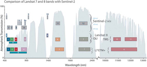
The red-edge lies between the red and NIR portions of the EM and is characterized by a sharp increase in vegetation reflectance (Filella and Penuelas 1994). Spectral bands in the red-edge portion have been found to be of importance in several application areas including agriculture, forestry, water, and LULC mapping. In agricultural applications, studies have pointed out the relevance of red-edge bands in estimating LAI (Filella and Penuelas 1994; Herrmann et al. 2011; Asam et al. 2013), plant chlorophyll and nitrogen content (Pinar and Curran 1996; Delegido et al. 2011; Clevers and Gitelson 2013), and discrimination of different crop types due to their sensitivity to different leaf and canopy structure (Ustuner et al. 2014; Immitzer, Vuolo, and Atzberger 2016; Radoux et al. 2016). These variables are important for determining crop conditions and estimating potential yield. Red-edge-derived vegetation indices were found to be important for early detection of stress symptoms of forest stands, ensuring timely intervention and protection of forest resources (Eitel et al. 2011; Dotzler et al. 2015). Schuster, Förster, and Kleinschmit (2012) found that the inclusion of red-edge bands in a LULC classification scheme impacted positively on vegetation classes and improved overall classification accuracy. In a land-cover mapping exercise, Zarco-Tejada and Miller (1999) noted that compared to all 16 spectral bands of a CASI (Compact Airborne Spectrographic Imager) image and Landsat TM data, the use of only red-edge spectral parameters of CASI produced better accuracy statistics.

Landscape heterogeneity in West Africa, and the resultant difficulty in separating LULC classes from remote-sensing data, has been pointed out by previous studies (Turner and Congalton 1998; Vancutsem et al. 2013; Lambert, Waldner, and Defourny 2016). In particular, the prevalence of small agricultural plots mosaicked with natural/semi-natural vegetation, diversity of cropping systems, and variable agronomic practices makes cropland mapping and crop-type discrimination a major challenge. However, recent crop mapping studies that utilized commercial sensors with a red-edge band (e.g., RapidEye) demonstrated the potential of the red-edge channel in improving the separability of LULC types in West Africa (Forkuor et al. 2014; Forkuor et al. 2015).

The present study aims at investigating the potential of S-2 data to improve the accuracy of LULC mapping in West Africa. In particular, the enhanced spectral (i.e., three red-edge bands) and spatial (10–20 m resolution) capabilities were tested to ascertain their contribution to improving the separability and detection of LULC types in a semi-arid environment. As previous LULC studies in West Africa have mostly used Landsat imagery, a comparison with L-8 images is performed to determine the added value of S-2. Finally, analysis is performed to explore how the two open-source high-resolution remote-sensing datasets (i.e., L-8 and S-2) can be used complementarily to increase the accuracy of LULC maps in West Africa.

Materials and methods

Study area

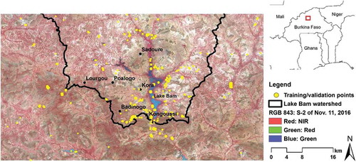
The study was conducted in the southern part of the watershed that encompasses Lake Bam, the largest natural lake in Burkina Faso and an important Ramsar wetland site (Figure 2). The site is located in the province of Bam in the Centre-Nord region of Burkina Faso. It falls in the Sudano-Sahelian agro-climatic zone which is characterized by a mono-modal rainfall regime. Annual rainfall from 1985 to 2015 ranged between 400 and 700 mm, with an average of 518 mm. Open shrubland are the dominant vegetation with isolated woody vegetation. Like most of Burkina Faso, subsistence agriculture is the main source of economic activity. Millet and sorghum are the dominant crops cultivated during the rainy season, while legumes (groundnuts and beans) are cultivated on a smaller scale. Land degradation, poor soil fertility, and frequent in-season droughts result in poor agricultural productivity, although soil management practices such as zai pits are frequently adopted by farmers. Zai pits are dug in the soil by farmers prior to the planting season and filled with organic matter to provide plant nutrients. The organic matter attracts termites, which bore channels that help break up the crusted soils (Roose, Kabore, and Guenat 1999). The existence of the lake permits local residents to cultivate vegetables along the lake during the long dry season from November to May. Crops cultivated include tomatoes, spring onions, green beans, green pepper, cabbage, and lettuce. Farmers use motor pumps to draw water from the lake to irrigate crops up to about 2 km from the banks of the lake. Previous studies have showed that irrigated area along the lake has increased in the last 5 years (Moser, Voigt, and Schoepfer 2014; Moser et al. 2016). This has led to increased pollution of the scarce resource (e.g., from pesticide and fertilizer usage) and increased erosion and subsequent sedimentation of the lake. The recent discovery of gold in the area, and the proliferation of small scale miners, will put a further strain on the lake’s resources and possibly aggravate the current level of pollution and environmental degradation.

Figure 2. Map of the study area showing the location of training and validation samples.

Data and pre-processing

Five multi-temporal L-8 and S-2 images, acquired in the same months of 2016, were analyzed in this study (Table 1). The L-8 images were downloaded free of charge from the USGS’ Earth Explorer portal (https://earthexplorer.usgs.gov/) while the S-2 images were obtained at no cost from the ESA’s Sentinels data hub (https://scihub.copernicus.eu/dhus/#/home). The L-8 scene falls on path 195 and row 51 while the S-2 scene falls in the tile 30PXV. All L-8 and S-2 images downloaded were cloud free over the study area. In importing the S-2 images, the spatial resolution of the red-edge and SWIR bands was resampled to 10 m using the nearest neighbor method to ensure integration with the 10-m visible and NIR bands.

Table 1. Dates of acquisition of L-8 and S-2 multi-temporal images analyzed.

Month	May	July	September	October	November
Landsat-8	28th	15th	1st	19th	4th
Sentinel-2	15th	14th	14th	23rd	11th

Studies have pointed out a temporary mis-registration between L-8 and S-2 due to residual geolocation errors contained in the L-8 reference framework, which is based on the Global Land Survey images (Storey et al. 2016; Yan et al. 2016). In order to correct for this defect, L-8 images were registered to their corresponding S-2 images using an initial set of ground control points (GCPs) selected from Google Earth. Based on these initial GCPs, an automatic point matching was performed to identify extra GCPs and tie points for an image-to-image registration. Root-mean-square errors obtained ranged from 0.19 to 0.24 pixels. To ensure integration of L-8 and S-2 for complementarity analysis, the L-8 images were resampled from its original 30 to 10 m resolution using the nearest neighbor method. For both L-8 and S-2, only the reflective bands in the visible, NIR, and SWIR sections of the EM and red edge (in the case of S-2) were used in subsequent analysis.

In addition to the spectral bands, some vegetation and land-cover-specific indices outlined in Table 2 were extracted. The vegetation indices, which have been found to be useful in vegetation studies (Rouse et al. 1973; Huete et al. 2002; Schuster, Förster, and Kleinschmit 2012; Kim and Yeom 2015), include normalized difference vegetation index (NDVI), red-edge dependent NDVI, and enhanced vegetation index (EVI). The land-cover-specific indices include modified normalized difference water index (MNDWI) and land surface water index for discriminating water bodies and normalized difference built-up index for built-up areas or settlements (Bhatti and Tripathi 2014). These indices were combined with the original spectral bands in the classification scheme.

Table 2. Vegetation and land-cover-specific spectral indices extracted from L-8 and S-2 images.

Name	Formulae	Reference
EVI		Huete et al. (2002)
EVI2		Jiang et al. (2008)
SAVI		Huete (1988)
NDVI		Rouse et al. (1973)
NDVI red edge1		Author’s own construct
NDVI red edge2		Author’s own construct
MNDWI		Xu (2006)
NDBI		Zha et al. (2003)
LSWI		Xiao et al. (2002)

EVI: Enhanced vegetation index; EVI2: enhanced vegetation index 2; SAVI: soil-adjusted vegetation index; NDVI: normalized difference vegetation index; MNDWI: modified normalized difference water index; NDBI: normalized difference built-up index; LSWI: land surface water index.

Reference data for the classification were collected during two field surveys in July and October 2016. A purposive sampling approach was adopted in mapping the land-use/land-cover classes of interest. These are (1) cereals, representing either millet, sorghum, or their intercropping; (2) legumes, which represent groundnuts, beans, or their intercropping; (3) shrubland; (4) forest; and (5) bare areas. A handheld GPS was used to map representative plots of these classes, keeping the minimum mapping area at 30 m × 30 m. Each plot was mapped by walking around it and saving waypoints at its corners. The GPS points were later processed into shapefile polygons using a standard GIS application. Reference data for two other classes – water/wetland and settlements – were on-screen digitized from false color composites of L-8 and S-2 images. The minimum mapping unit of 30 m × 30 m was applied here as well. These classes were not mapped on the field due to the ease of identifying them on false color composites. In total, reference data for seven LULC classes were generated for subsequent analysis.

Methodology

Figure 3 gives an overview of the methodological approach adopted for this study. Five classification runs (experiments) with different data configurations were conducted to achieve the objectives of the study (Table 3). Each experiment consisted of the spectral bands of the respective images and their corresponding spectral indices. Three well-known machine-learning classification algorithms – random forest (RF) (Breiman 2001), support vector machines (SVM) (Mountrakis, Im, and Ogole 2011), and stochastic gradient boosting (SGB) (Friedman 2002) – were used to classify the different data configurations and their results were compared. These three algorithms were selected due to their high performance reported by several studies (Ogutu, Piepho, and Schulz-Streeck 2011; Li, Im, and Beier 2013; Freeman et al. 2016; Forkuor et al. 2017).

Table 3. Different data configurations (experiments) that were classified in order to compare L-8 and S-2.

Name	Number of features/bands	Spectral bands involved	Objective
Landsat-8	65	All L-8 bands and associated indices	To determine LULC mapping accuracies obtainable from multi-temporal L-8 data
Sentinel-2	95	All S-2 bands and associated indices	To determine LULC mapping accuracies obtainable from multi-temporal S-2 data
Sentinel-2 subset	65	Common S-2 visible, NIR and SWIR bands to L-8 and associated indices	To enable a direct comparison between S-2 and L-8 in terms of LULC mapping accuracies
Red-edge only	25	Red-edge bands and associated indices	To determine LULC mapping accuracies obtainable from only red-edge bands
Landsat-8 plus red-edge	90	All L-8, S-2 red-edge bands and associated indices	To determine mapping accuracy when S-2 red-edge bands are combined with L-8 data

Figure 3. Overview of methodological approach.

The caret (classification and regression training) package (Kuhn et al. 2017) in the R statistical and programming environment (R Core Team 2015) was used to implement the three classification algorithms. The “kernlab,” “GBM,” and “randomForest” libraries of the caret package were used for SVM, SGB, and RF, respectively (Kuhn et al. 2017). The caret package was chosen due to its ability to streamline the model building and evaluation process of different classification and regression algorithms (Kuhn et al. 2017). The package reduces the complexity associated with model tuning by first iterating over a range of values of model parameters and then selecting the parameter combination that gives the best performance for building a final model.

In implementing the classification algorithms, reference samples were derived by overlaying the reference data on the image data and extracting the underlying values. For each LULC class, a condition was set to extract a maximum of 300 samples points from all possible samples falling within polygons of that class. Sampling was done in such a way that within a resampled L-8 pixel having nine (3 × 3) 10 m pixels, only one pixel was sampled to avoid duplicating values in an original 30-m L-8 pixel. A total of 1654 points were sampled for all classes. The maximum number of samples (i.e., 300) was not achieved for some of the classes (e.g., settlements) due to their limited extent. The extracted sampling points were split into a 50–50% training and validation samples using a stratified random split (via the “createDataPartition” function of the caret package). In building a model, optimal tuning parameters were first determined based on multiple resampling of the training data and an evaluation of the effect of different parameter sets on model performance using cross-validation. Here, 10 random partitions of the training data with 5 repetitions (i.e., via the trainControl function of caret) were used to automatically determine the optimal tuning parameters for the 3 algorithms. The tuning parameters considered are the number of predictors/variables to be tried at each split (mtry) for RF, the penalty parameter C, which controls the trade-off between training error and model complexity for SVM, and the number of trees, interaction depth (maximum nodes per tree), shrinkage (learning rate), and n.minobsinnode (minimum number of observations in a trees’ terminal nodes) for SGB (Kuhn et al. 2017). Shrinkage and n.minobsinnode were kept constant for SGB.

To ensure that the same folds (random samples) were used in each of the three algorithms and permit a direct comparison of their results, the random number seeds were initialized to the same value before each model was trained (via the “train” function). The optimal parameter set was then used to generate the final model which was subsequently validated using the 50% testing samples. Validation of each model’s results with the testing samples produced accuracy assessment statistics such as overall accuracy, kappa statistic, user’s and producer’s accuracy, sensitivity, and specificity (Kuhn et al. 2017). The F1-score (Halder, Ghosh, and Ghosh 2009), a composite measure of user’s and producer’s accuracies, was calculated for each class and experiment for subsequent comparison. Accuracy estimates from the model generation process were noted. In addition to the accuracy estimates, the contribution of the different spectral bands and indices in generating the respective models were determined using variable importance measures. These measures were derived from the RF models because apart from estimating the contribution of variables (i.e., spectral bands and indices) to the obtained overall accuracy of the model, RF further provides information on the contribution of each variable to discriminating the different LULC classes. The Mean Decrease Gini (MDG) variable importance measure of RF (Breiman 2002; Liaw and Wiener 2002; Calle and Urrea 2011) was used. MDG provides a measure of the role a variable plays in partitioning the training data into the defined LULC classes during the model building process. A high MDG indicates a higher variable importance and vice versa.

Results and discussion

Classification accuracy of LULC maps

Table 4 presents a summary of the results (overall accuracy and kappa coefficient) obtained when the generated models were validated using the 50% test data (via the “predict” and “confusionMatrix” functions in caret). With the exception of the SVM and SGB classifications of L-8, overall accuracies of 90% or greater were obtained for all experiments with the three algorithms. SGB and RF generally performed better than SVM, achieving the highest overall accuracy in three and two experiments, respectively. However, SVM produced slightly higher accuracies than RF in two experiments, while SGB consistently performed better than SVM. RF showed some inconsistency when it produced a lower overall accuracy for the classification of S-2 (95 predictors: 92.5%) compared to S-2 subset (65 predictors: 93.1%), while overall accuracies obtained by SVM and SGB increased from classification of S-2 subset to S-2. Although the RF algorithm is known to be less sensitive to tuning parameters, i.e., mtry – number of predictors tried at each split and ntrees – number of trees built, the final choice of mtry (48) in the classification of S-2 is a possible reason for the low accuracy.

Table 4. Overall accuracy and kappa coefficient of the various experiments or data configurations classified.

	Overall accuracy			Kappa coefficient
Experiment/Classification	RF	SVM	SGB	RF	SVM	SGB
Landsat-8	90.5	88.9	89.2	0.886	0.867	0.871
Sentinel-2 subset	93.1	92.9	93.6	0.918	0.915	0.923
Sentinel-2	92.5	93.4	94.3	0.910	0.920	0.932
Red-edge only	92.4	91.1	91.7	0.909	0.893	0.900
Landsat plus red edge	92.3	92.7	93.4	0.908	0.913	0.921

The reported mixed performance of the algorithms has been noted by previous studies that compared the accuracies of different machine-learning algorithms (MLAs). For example, Inglada et al. (2015) compared four MLAs – RF, SVM, SGB, and decision trees – in delivering an operational crop mapping. They showed that RF performed better than the other algorithms. Rodriguez-Galiano et al. (2012) also found RF to outperform SVM, regression trees, and artificial neural networks in mineral prospectivity modeling. On the other hand, Statnikov, Wang, and Aliferis (2008) performed a rigorous evaluation of SVM and RF and concluded that SVM produced better results than RF. Ogutu, Piepho, and Schulz-Streeck (2011) revealed that SGB performs better than SVM and RF in predicting genomic breeding values. Forkuor et al. (2017) found RF to perform marginally better than SGB and SVM when they compared the algorithms for predicting soil properties at local scale. What is common in most of these studies is that the differences in accuracies produced by the MLAs were often minimal and sometimes statistically insignificant. Adam et al. (2014), for instance, reported a higher overall accuracy for RF (93.07%) than SVM (91.80%), although a McNemar’s test showed that the difference was statistically insignificant. Similarly, Freeman et al. (2016) found the performances of RF and SGB to be remarkably similar in mapping LULC in four study sites in the United States. In this study, a simple t-test conducted using the internal statistics of the generated models (via the “resamples” and “diff” functions in caret) revealed that the difference in accuracy between SGB and RF was mostly statistically insignificant. Thus, the two models could be considered comparable in classification performance. On the other hand, the accuracy difference between RF and SVM and that between SGB and SVM were mostly statistically significant. Due to similarities in the performance of SGB and RF, subsequent discussions are based on the accuracy estimates produced by the SGB model. However, discussions on the contribution of the S-2 red-edge bands to mapping the studied LULC classes were based on variable importance measures obtained from the generated RF models.

Table 4 reveals that all S-2-related experiments produced better accuracy estimates than L-8 only. The highest overall accuracy was achieved with the classification of all S-2 bands (94.3%), which represents an improvement of about 5% over that achieved with all L-8 bands. Classification of S-2 bands that are common to L-8 also resulted in better estimates (93.6%) than L-8, recording an improvement in overall accuracy of about 4%. Other studies that compared the accuracy of L-8 and S-2 for LULC obtained similar results. Topaloğlu, Sertel, and Musaoğlu (2016), for example, compared the similar bands between L-8 and S-2 in a LULC classification study and noted that S-2 produced an overall accuracy of 3–6% higher than that obtained by L-8. Thus, apart from the added spectral bands in S-2, the S-2 bands common to L-8 possess spectral capabilities that yield slightly better classification accuracies than L-8. The spectral properties of S-2 produced a better classification of built-up areas when it was compared with that of Landsat and Sentinel-1 imagery in northeastern Italy (Pesaresi et al. 2016). Although the spectral bands of S-2 and L-8 are placed at similar locations in the EM, S-2 has relatively narrower bands, which could improve the detection and discrimination of specific land surface properties or LULC types.

Comparing the classification accuracy of L-8 only (89.2%) with that of L-8 and the S-2 red-edge bands (93.4%) suggests a reasonably positive influence of the red-edge bands on the accuracy of LULC mapping in the study area. The inclusion of the red-edge bands increased overall accuracy by about 4%. The variable importance plot (from the SGB model) of the L-8 plus red-edge experiment (Figure 4a) shows that five red-edge bands were included in the first 10 most important variables. Band 5 (RE1) was found to be among the first five important variables. This result indicates some advantages in the complementary use of data from L-8 and S-2.

Figure 4. Variable importance plot for the classification involving (a) L-8 and S-2 red-edge bands and (b) all S-2 bands.

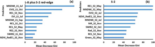
Comparison of the classification accuracy of S-2 subset (93.6%) with that of S-2 (94.3%), on the other hand, suggests a minimal influence of the red-edge bands in the latter experiment. Here, the inclusion of the red-edge to the other S-2 bands increased overall accuracy by only 0.7%. A possible explanation for this minimal influence is that the spectral bands within the S-2 subset were able to achieve optimal separability of the classes of interest, resulting in less impact of the red-edge bands on accuracy. However, the variable importance plot (Figure 4b) showed a red-edge band (RE1 of May) as the most important variable, while the NDVI red edge of November came up amongst the first five important variables.

Results obtained when only red-edge bands were classified present the strongest evidence of the importance of the red-edge channel in vegetation analysis and LULC mapping in general. Although this experiment consisted of only 25 features (see Table 3), the achieved overall accuracy (91.7%) was better than L-8 (89.2%) and comparable to S-2 subset (93.6%). This means that the information in the three S-2 red-edge bands is almost as important as the other seven visible, NIR, and SWIR bands. Zarco-Tejada and Miller (1999) made similar observations when they tested data from the CASI for land-cover mapping in the BOReal Ecosystem-Atmosphere Study. They compared the use of only red-edge spectral parameters of CASI against all 16 CASI channels and a Landsat TM-based classification. Classification with the red-edge spectral parameters alone produced a kappa coefficient that was 16% and 23% better than that obtained when all 16 CASI channels and Landsat TM, respectively, were classified. The superiority of the S-2 red-edge bands over L-8 in terms of classification accuracy demonstrates the need for multi-sensor approaches in improving LULC mapping in data scarce regions.

Classification accuracy of LULC classes

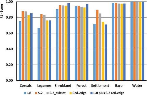
Tables 5–7 show the confusion matrices of three of the experiments based on the SGB classification algorithm while Figure 5 summarizes the accuracy (F1-score) with which the LULC classes were mapped in all five experiments. Similar to results presented in Table 4, the classification based on L-8 produced the lowest accuracies (F1-score) for the crop classes (i.e., 75% for cereals and 67% for legumes). Table 5 indicates that spectral confusion between the crop classes was the main reason for the recorded low F1-score, while confusion between the crop and vegetative classes were minimal. Compared to the L-8 only classification, those of S-2 subset, S-2, and red edge only produced a significant improvement in F1-score by 8–18% for the crop classes. Combination of the S-2 red-edge bands with the L-8 bands (L-8 plus red edge) also increased the F1-score of the crop classes by 10% compared to L-8 only (Table 6). The observed improvements in F1-score of the crop classes in all experiments, including the S-2 red-edge bands, signify the importance of red-edge bands to crop classification in the study area. More importantly, the possibility of obtaining improved accuracies when the S-2 red-edge bands are combined with L-8 is promising for future research in agricultural land-use mapping. Unlike the crop classes, there was relatively low spectral confusion between the vegetative classes (i.e., forest and shrubland) in all experiments. Consequently, the inclusion of red-edge bands produced relatively lower increments in F1-score.

Table 5. Confusion matrix for the SGB classification of L-8 bands and indices only.

		Groundtruth
	Classes	Bare	Cereals	Legumes	Shrubland	Forest	Settlements	Water	Total
Classification	Bare	148	1		2				151
	Cereals		88	23	1	5	1		118
	Legumes	1	19	57	2		8		87
	Shrubland		7	4	135	2			148
	Forest		1		7	142			150
	Settlements	1			3	1	18		23
	Water							150	150
	Total	150	116	84	150	150	27	150	827
	PA	0.99	0.76	0.68	0.90	0.95	0.67	1.00
	UA	0.98	0.75	0.66	0.91	0.95	0.78	1.00
	F1-score	0.98	0.75	0.67	0.91	0.95	0.72	1.00

 Bold values represent the total number of groundtruth and classified pixels considered in the accuracy assessment

Table 6. Confusion matrix for the SGB classification of L-8 and S-2 red-edge bands.

		Groundtruth
	Classes	Bare	Cereals	Legumes	Shrubland	Forest	Settlements	Water	Total
Classification	Bare	146	1	2					149
	Cereals	3	102	14	1	3			123
	Legumes		12	66			11		89
	Shrubland				147	2			149
	Forest		1	1	2	145			149
	Settlements	1		1			16		18
	Water							150	150
	Total	150	116	84	150	150	27	150	827
	PA	0.97	0.88	0.79	0.98	0.97	0.59	1.00
	UA	0.98	0.83	0.74	0.99	0.97	0.89	1.00
	F1-score	0.98	0.85	0.76	0.98	0.97	0.71	1.00

 Bold values represent the total number of groundtruth and classified pixels considered in the accuracy assessment

Table 7. Confusion matrix for the SGB classification of S-2 bands and indices only.

		Groundtruth
	Classes	Bare	Cereals	Legumes	Shrubland	Forest	Settlements	Water	Total
Classification	Bare	147					1		148
	Cereals	1	102	7	2	4			116
	Legumes	2	13	75			4		94
	Shrubland			1	141	3			145
	Forest		1	1	7	143			152
	Settlements						22		22
	Water							150	150
	Total	150	116	84	150	150	27	150	827
	PA	0.98	0.88	0.89	0.94	0.95	0.81	1.00
	UA	0.99	0.88	0.80	0.97	0.94	1.00	1.00
	F1-score	0.99	0.88	0.84	0.96	0.95	0.90	1.00

 Bold values represent the total number of groundtruth and classified pixels considered in the accuracy assessment

Figure 5. Class-specific accuracies for the five experiments obtained from the SGB classifications (L-8 = Landsat-8; S-2 = Sentinel-2; S-2_subset = S-2 bands common to L-8).

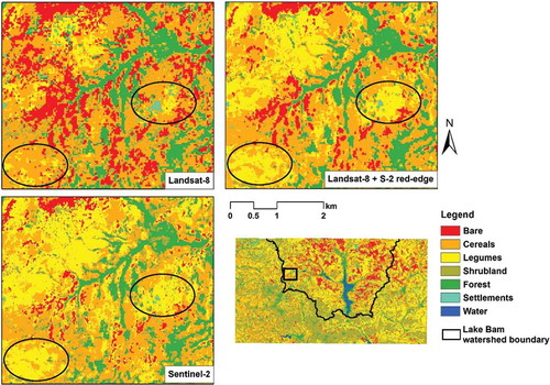
Figure 6 provides detailed views of the SGB classifications of L-8 only, L-8 plus S-2 red-edge bands, and S-2 only. In West Africa, different crops are often cultivated in a continuum without clear farm/plot boundaries. Consequently, there is lack of a cropland structure, which is evident in the figure. The figure demonstrates the limited separability between the crop classes on the L-8 only classification, while an improvement in the separability of the two classes is evident in the L-8 plus red edge and S-2 classifications (black ellipses). On the other hand, the figure shows a similar pattern for the vegetative classes on all three classifications. A detailed look at the figure demonstrates the superior spatial resolution of S-2, which is evident in both the L-8 plus S-2 red-edge and S-2 classifications. The boundaries of LULC units in these two maps are sharper than in the L-8 map.

Figure 6. Detailed views of the SGB classifications of L-8 only, L-8 plus S-2 red-edge bands, and S-2 only. Black ellipses show areas where L-8 plus S-2 red edge and S-2 achieved improved separation compared to L-8 only.

Contribution of red edge to LULC mapping

Figure 7 presents variable importance plots for five LULC classes derived from the classification of L-8 plus S-2 red-edge bands. These plots were generated from the RF model due to difficulty in deriving class-specific variable importance measures from the SGB model. The plots are meant to further demonstrate the advantages of the S-2 red-edge bands in LULC classification and the potential of multi-sensor approaches in future mapping.

Figure 7. Variable importance measures of five LULC classes derived from the random forest classification of L-8 plus S-2 red-edge bands.

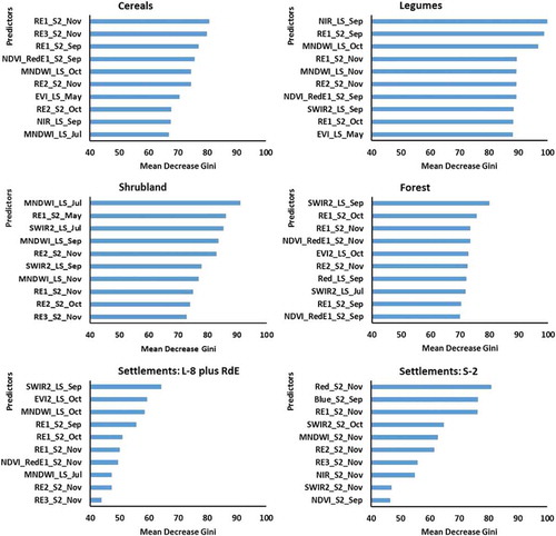
The variable importance plots of cereals and legumes (first row) indicate that the red-edge bands significantly contributed to improving the F1-score of the crop classes as indicated in Figure 5. In the case of cereals, the first 4 most important predictors were red-edge bands and indices, while 6 out of the 10 most important predictors were red-edge bands. Similarly, 5 out of the 10 most important predictors were red-edge bands and indices for the legumes class. In both cases, S-2 band 5 (RE1) and related indices came up prominently. The plots further reveal that images acquired late in the cropping season (i.e., September–November) were most important in the discrimination of the crop classes. This is in line with previous studies that investigated similar crops in other parts of West Africa (Forkuor 2014; Forkuor et al. 2014). Immitzer, Vuolo, and Atzberger (2016) also underscored the importance of the S-2 red-edge bands in crop classification in their analysis of a mono-temporal S-2 image over an Austrian agricultural area. Amongst the five most important S-2 bands for crop discrimination, they found that two were red-edge bands, with S-2 band 5 (RE1) being the most important band. Radoux et al. (2016) also confirmed the importance of the S-2 red-edge bands for crop classification, although contrary to the study described in this article and Immitzer, Vuolo, and Atzberger (2016), they found bands 6 and 7 (RE2 and RE3) to perform better than band 5 (RE1). On the other hand, Radoux et al. (2016) confirmed the importance of the SWIR band for crop classification as noted by Immitzer, Vuolo, and Atzberger (2016), although this was not evident in the results of this study. These slight differences in results can be attributed to differences in the crop classes investigated, and in the case of SWIR, differences in sensors (L-8 and S-2). Nonetheless, like previous studies that examined S-2, the results of this study clearly demonstrated that, compared to other sensors that have a single red-edge band (e.g., RapidEye), the three red-edge bands of S-2 will increase chances of improving the classification of a wide range of crops as well as the retrieval of important biophysical parameters (Inglada et al. 2012; Richter et al. 2012; Clevers and Gitelson 2013).

The results of this study have further confirmed the importance of the red-edge bands for vegetation mapping as indicated by previous studies (Schuster, Förster, and Kleinschmit 2012; Ramoelo et al. 2015; Immitzer, Vuolo, and Atzberger 2016). Compared to the crop classes, however, including the red-edge bands (i.e., in combination with L-8) gave relatively lower increments in the class-wise accuracy of the vegetative classes. F1-scores of shrubland and forest increased by 8% and 2%, respectively, when L-8 and S-2 red-edge bands were classified (compared to L-8 only). S-2 was found to perform marginally better than L-8 when both sensors were tested for estimating canopy cover and LAI in Finland (Korhonen, Packalen, and Rautiainen 2017). Band 5 (RE1) was noted as a possible explanation for the marginally better performance of S-2. Red-edge bands were found to be useful for discriminating rangeland management practices when simulated HyspIRI, L-8, S-2, and VENµS spectral data were compared (Sibanda, Mutanga, and Rouget 2016a). Other studies alluded to the importance of Landsat’s SWIR bands in the study of forest vegetation and ecological applications in general (Eklundh, Harrie, and Kuusk 2001; Cohen and Goward 2004; Vogelmann, Tolk, and Zhu 2009). Consequently, classifications involving L-8 achieved high F1-scores for the forest class. The variable importance plot of the forest class shows the SWIR2 band of L-8 as the most important predictor, confirming the importance of SWIR bands for forest mapping. Nonetheless, out of the top 10 important predictors for the forest class, 6 were S-2 red-edge bands, with 3 being in the top 5. Thus, although the inclusion of the red-edge bands did not lead to a substantial increase in F1-score, their importance and application to forest mapping has been clearly shown in previous studies (Schuster, Förster, and Kleinschmit 2012; Ramoelo et al. 2015; Immitzer, Vuolo, and Atzberger 2016). In the case of shrubland (also a vegetative class), integration of the red-edge bands resulted in an F1-score increment of 8% (compared to L-8 only). Interestingly, the most important predictor for this class was found to be the MNDWI. A possible explanation is that this index is derived from the visible (green) and SWIR portions of the EM (SWIR1), as the latter is generally useful for vegetation studies (Liu, Wimberly, and Dwomoh 2016). Five red-edge bands, however, came up in the top 10 most important predictors for shrubland. Collectively, results of this study confirmed findings of other studies which highlighted the value of red-edge and SWIR bands of S-2 in vegetation mapping (Schuster, Förster, and Kleinschmit 2012; Ramoelo et al. 2015).

Figure 5 reveals that, compared to the L-8 only classification, combining the S-2 red-edge bands with L-8 did not improve the F1-score of the settlements, bare, and water classes. However, classification of S-2 and S-2 subset achieved an improvement of 18% and 13%, respectively, in the F1-score of the settlements class (i.e., compared to L-8 only). The variable importance plot of the settlements class based on the classification of S-2 (Figure 7) shows the S-2 visible bands of red and blue as the two most important variables in discriminating the settlements class from other classes. This could partly be attributed to the spatial resolution of the visible bands (10 m), as the study area contains rural settlements with relatively small buildings. Nonetheless, one red-edge band (Band 5 – RE1) came up in the first five most important predictors, signifying some influence of the red-edge band in improving the accuracy of the settlements class.

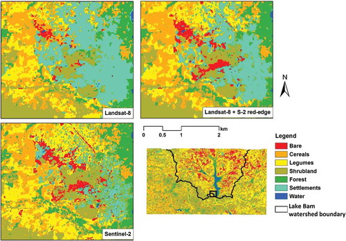
Figure 8 shows detailed views of the Kongoussi township based on the classification of three data configurations. There is evidence that the spatial resolution limitations of L-8 result in a blurred representation of the township compared to the S-2 classification that shows improved spatial detail, thanks to the presence of the 10-m blue and red bands.

Figure 8. Detailed views of the SGB classifications of Landsat-8 only, L-8 plus S-2 red-edge bands, and S-2 only on the main Kongoussi township.

Conclusion

The recent launch of the S-2 sensor by the ESA will increase open access to moderate-to-high spatial resolution imagery for multiple applications. Compared to the spatial, spectral, and temporal resolution of satellites in the Landsat missions, the S-2 sensor presents new and interesting properties. Notable among these is the addition of three bands in the red-edge portion of the EM (Figure 1). This study sought to compare the LULC mapping accuracies obtainable from S-2 and L-8 and investigated the added value of the red-edge bands of S-2 in rural Burkina Faso. Five experiments involving different data configurations (i.e., L-8, S-2, S-2_subset, red-edge only, L-8 plus S-2 red-edge) were setup and classified using three MLAs – RF, SVM, and SGB.

SGB and RF performed slightly better than SVM in most cases. Differences in the accuracy estimates of SGB and RF were generally statistically insignificant, while those of SGB and SVM and RF and SVM were mostly statistically significant. Classification of all S-2 bands as well as S-2 bands common to L-8 produced an overall accuracy of 5% and 4% better than L-8. It was found that classification of the S-2 red-edge bands alone produced better and comparable results to L-8 and the other S-2 bands (i.e., visible, NIR, and SWIR), respectively. The combination of L-8 and S-2 red-edge bands resulted in a 4% accuracy improvement over that of L-8, while the accuracy of crop classes improved by at least 10%. Variable importance plots derived from the L-8 plus S-2 red-edge bands revealed that, compared to L-8 only classification, accuracy improvements in most LULC classes were attributable to the S-2 red-edge bands, especially S-2 Band 5.

Results of this study demonstrate the added value of the S-2 red-edge bands to improving LULC mapping and encourage multi-sensoral approaches (i.e., combined use of S-2 and L-8) for future research. Subsequent studies should investigate possibilities of further improvements in LULC mapping for data poor regions such as West Africa by integrating Sentinel-1 data.

Highlights

• High resolution imagery required for improved land use and land cover (LULC)

• Sentinel-2 provides open source high spatial, temporal and spectral data

• Potential of Sentinel-2 to improve LULC in data poor regions investigated

• Sentinel-2’s red-edge bands improves discrimination of LULC classes

• Complementary use of Sentinel-2 and Landsat8 found to be beneficial for LULC mapping

Acknowledgements

Authors will like to thank Mr. Francis Dwomoh of the Geospatial Sciences Center of Excellence for his critical comments on an earlier version of the manuscript. We will also like to thank the anonymous reviewers whose comments and suggestions improved the quality of the presentation.

Disclosure statement

No potential conflict of interest was reported by the authors.

Additional information

Funding

This article was supported by European Space Agency under Tiger Project 402 and German Federal Ministry of Education and Research under 01LG1001A

References

- Adam, E., O. Mutanga, J. Odindi, and E. M. Abdel-Rahman. 2014. “Land-Use/Cover Classification in a Heterogeneous Coastal Landscape Using RapidEye Imagery: Evaluating the Performance of Random Forest and Support Vector Machines Classifiers.” International Journal of Remote Sensing 35 (10): 3440–3458. doi:10.1080/01431161.2014.903435.
- Ahmadian, N., S. Ghasemi, J.-P. Wigneron, and R. Zölitz. 2016. “Comprehensive Study of the Biophysical Parameters of Agricultural Crops Based on Assessing Landsat 8 OLI and Landsat 7 ETM+ Vegetation Indices.” GIScience & Remote Sensing 53 (3): 337–359. doi:10.1080/15481603.2016.1155789.
- Asam, S., H. Fabritius, D. Klein, C. Conrad, and S. Dech. 2013. “Derivation of Leaf Area Index for Grassland within Alpine Upland Using Multi-Temporal RapidEye Data.” International Journal of Remote Sensing 34 (23): 8628–8652. doi:10.1080/01431161.2013.845316.
- Bhatti, S. S., and N. K. Tripathi. 2014. “Built-Up Area Extraction Using Landsat 8 OLI Imagery.” GIScience & Remote Sensing 51 (4): 445–467. doi:10.1080/15481603.2014.939539.
- Breiman, L. 2001. “Random Forests.” Machine Learning 45 (1): 5–32. doi:10.1023/A:1010933404324.
- Breiman, L., 2002. Manual on Setting Up, Using, and Understanding Random Forests V3.1 [Online]. http://oz.berkeley.edu/users/breiman/
- Calle, M. L., and V. Urrea. 2011. “Letter to the Editor: Stability of Random Forest Importance Measures.” Briefings in Bioinformatics 12 (1): 86–89. doi:10.1093/bib/bbq011.
- Chen, J., J. Chen, A. Liao, X. Cao, L. Chen, X. Chen, C. He, et al. 2015. “Global Land Cover Mapping at 30m Resolution: A POK-based Operational Approach.” ISPRS Journal of Photogrammetry and Remote Sensing 103: 7–27. doi:10.1016/j.isprsjprs.2014.09.002.
- Clevers, J. G. P. W., and A. A. Gitelson. 2013. “Remote Estimation of Crop and Grass Chlorophyll and Nitrogen Content Using Red-Edge Bands on Sentinel-2 and −3.” International Journal of Applied Earth Observation and Geoinformation 23: 344–351. doi:10.1016/j.jag.2012.10.008.
- Cohen, W. B., and S. N. Goward. 2004. “Landsat’s Role in Ecological Applications of Remote Sensing.” BioScience 54 (6): 535. doi:10.1641/0006-3568(2004)054[0535:LRIEAO]2.0.CO;2.
- Delegido, J., J. Verrelst, L. Alonso, and J. Moreno. 2011. “Evaluation of Sentinel-2 Red-Edge Bands for Empirical Estimation of Green LAI and Chlorophyll Content.” Sensors 11 (12): 7063–7081. doi:10.3390/s110707063.
- Dotzler, S., J. Hill, H. Buddenbaum, and J. Stoffels. 2015. “The Potential of EnMAP and Sentinel-2 Data for Detecting Drought Stress Phenomena in Deciduous Forest Communities.” Remote Sensing 7 (10): 14227–14258. doi:10.3390/rs71014227.
- Drusch, M., U. Del Bello, S. Carlier, O. Colin, V. Fernandez, F. Gascon, B. Hoersch, et al. 2012. “Sentinel-2: ESA’s Optical High-Resolution Mission for GMES Operational Services.” Remote Sensing of Environment 120: 25–36. doi:10.1016/j.rse.2011.11.026.
- Eitel, J. U. H., L. A. Vierling, M. E. Litvak, D. S. Long, U. Schulthess, A. A. Ager, D. J. Krofcheck, and L. Stoscheck. 2011. “Broadband, Red-Edge Information from Satellites Improves Early Stress Detection in a New Mexico Conifer Woodland.” Remote Sensing of Environment 115 (12): 3640–3646. doi:10.1016/j.rse.2011.09.002.
- Eklundh, L., L. Harrie, and A. Kuusk. 2001. “Investigating Relationships between Landsat ETM+ Sensor Data and Leaf Area Index in a Boreal Conifer Forest.” Remote Sensing of Environment 78 (3): 239–251. doi:10.1016/S0034-4257(01)00222-X.
- Filella, I., and J. Penuelas. 1994. “The Red Edge Position and Shape as Indicator of Plant Chlorophyll Content, Biomass and Hydric Status.” International Journal Remote Sensing 15 (7): 1459–1470. doi:10.1080/01431169408954177.
- Forkuor, G. 2014. “Agricultural Land Use Mapping in West Africa Using Multi-Sensor Satellite Imagery.” University of Wuerzburg. http://opus.bibliothek.uni-wuerzburg.de/frontdoor/index/index/docId/10868.
- Forkuor, G., C. Conrad, M. Thiel, T. Landmann, and B. Barry. 2015. “Evaluating the Sequential Masking Classification Approach for Improving Crop Discrimination in the Sudanian Savanna of West Africa.” Computers and Electronics in Agriculture 118: 380–389. doi:10.1016/j.compag.2015.09.020.
- Forkuor, G., C. Conrad, M. Thiel, T. Ullmann, and E. Zoungrana. 2014. “Integration of Optical and Synthetic Aperture Radar Imagery for Improving Crop Mapping in Northwestern Benin, West Africa.” Remote Sensing 6 (7): 6472–6499. doi:10.3390/rs6076472.
- Forkuor, G., O. K. L. Hounkpatin, G. Welp, and M. Thiel. 2017. “High Resolution Mapping of Soil Properties Using Remote Sensing Variables in South-Western Burkina Faso: A Comparison of Machine Learning and Multiple Linear Regression Models.” Plos One 12 (1): 1–21. doi:10.1371/journal.pone.0170478.
- Freeman, E. A., G. G. Moisen, J. W. Coulston, and B. T. Wilson. 2016. “Random Forests and Stochastic Gradient Boosting for Predicting Tree Canopy Cover: Comparing Tuning Processes and Model Performance 1.” Canadian Journal of Forest Research 46 (3): 323–339. doi:10.1139/cjfr-2014-0562.
- Friedl, M. A., D. Sulla-Menashe, B. Tan, A. Schneider, N. Ramankutty, A. Sibley, and X. Huang. 2010. “MODIS Collection 5 Global Land Cover: Algorithm Refinements and Characterization of New Datasets.” Remote Sensing of Environment 114 (1): 168–182. doi:10.1016/j.rse.2009.08.016.
- Friedman, J. H. 2002. “Stochastic Gradient Boosting.” Computational Statistics & Data Analysis 38 (4): 367–378. doi:10.1016/S0167-9473(01)00065-2.
- Fritz, S., L. See, and F. Rembold. 2010. “Comparison of Global and Regional Land Cover Maps with Statistical Information for the Agricultural Domain in Africa.” International Journal of Remote Sensing 31 (9): 2237–2256. doi:10.1080/01431160902946598.
- Halder, A., A. Ghosh, and S. Ghosh. 2009. “Aggregation Pheromone Density Based Pattern Classification.” Fundamenta Informaticae 92: 345–362.
- Hansen, M. C., P. V. Potapov, R. Moore, M. Hancher, S. A. Turubanova, A. Tyukavina, D. Thau, et al. 2013. “High-Resolution Global Maps of 21st-Century Forest Cover Change.” Science 342: 6160. doi:10.1126/science.1244693.
- Herrmann, I., A. Pimstein, A. Karnieli, Y. Cohen, V. Alchanatis, and D. J. Bonfil. 2011. “LAI Assessment of Wheat and Potato Crops by Venμs and Sentinel-2 Bands.” Remote Sensing of Environment 115 (8): 2141–2151. doi:10.1016/j.rse.2011.04.018.
- Huete, A., K. Didan, T. Miura, E. Rodriguez, X. Gao, and L. Ferreira. 2002. “Overview of the Radiometric and Biophysical Performance of the MODIS Vegetation Indices.” Remote Sensing of Environment 83 (1–2): 195–213. doi:10.1016/S0034-4257(02)00096-2.
- Huete, A.R. 1988. “A Soil-adjusted Vegetation Index (Savi).” Remote Sensing Of Environment 25 (3): 295–309. doi: 10.1016/0034-4257(88)90106-X.
- Immitzer, M., F. Vuolo, and C. Atzberger. 2016. “First Experience with Sentinel-2 Data for Crop and Tree Species Classifications in Central Europe.” Remote Sensing 8: 166. doi:10.3390/rs8030166.
- Inglada, J., J.-F. Dejoux, O. Hagolle, and G. Dedieu. 2012. “Multi-Temporal Remote Sensing Image Segmentation of Croplands Constrained by a Topographical Database.” In 2012 IEEE International Geoscience and Remote Sensing Symposium, 6781–6784. IEEE. doi:10.1109/IGARSS.2012.6352607.
- Inglada, J., M. Arias, B. Tardy, O. Hagolle, S. Valero, D. Morin, G. Dedieu, et al. 2015. “Assessment of an Operational System for Crop Type Map Production Using High Temporal and Spatial Resolution Satellite Optical Imagery.” Remote Sensing 7 (9): 12356–12379. doi:10.3390/rs70912356.
- Jiang, Z., A.R. Huete, K. Didan, and T. Miura. 2008. “Development Of A Two-band Enhanced Vegetation Index Without A Blue Band.” Remote Sensing Of Environment 112 (10): 3833–3845. doi: 10.1016/j.rse.2008.06.006.
- Kim, H.-O., and J.-M. Yeom. 2015. “Sensitivity of Vegetation Indices to Spatial Degradation of RapidEye Imagery for Paddy Rice Detection: A Case Study of South Korea.” GIScience & Remote Sensing 52 (1): 1–17. doi:10.1080/15481603.2014.1001666.
- Korhonen, L., P. Packalen, and M. Rautiainen. 2017. “Comparison of Sentinel-2 and Landsat 8 in the Estimation of Boreal Forest Canopy Cover and Leaf Area Index.” Remote Sensing of Environment 195: 259–274. doi:10.1016/j.rse.2017.03.021.
- Kuhn, M., J. Wing, S. Weston, A. Williams, C. Keefer, A. Engelhardt, T. Cooper, et al., 2017. Caret: Classification and Regression Training [Online]. R Package Version 6.0-76. http://cran.r-project.org/package=caret.
- Lambert, M., F. Waldner, and P. Defourny. 2016. “Cropland Mapping over Sahelian and Sudanian Agrosystems : A Knowledge-Based Approach Using PROBA-V Time Series at 100-M.” Remote Sensing 8 (232): 1–23. doi:10.3390/rs8030232.
- Leroux, L., A. Jolivot, A. Bégué, D. L. Seen, and B. Zoungrana. 2014. “How Reliable Is the {MODIS} Land Cover Product for Crop Mapping {Sub-Saharan} Agricultural Landscapes?” Remote Sensing 6 (9): 8541–8564. doi:10.3390/rs6098541.
- Li, M., J. Im, and C. Beier. 2013. “Machine Learning Approaches for Forest Classification and Change Analysis Using Multi-Temporal Landsat TM Images over Huntington Wildlife Forest.” GIScience & Remote Sensing 50 (4): 361–384.
- Liaw, A., and M. Wiener. 2002. “Classification and Regression by Random Forest.” R News 2 (3): 18–22.
- Liu, Z., M. Wimberly, and F. Dwomoh. 2016. “Vegetation Dynamics in the Upper Guinean Forest Region of West Africa from 2001 to 2015.” Remote Sensing 9 (1): 5. doi:10.3390/rs9010005.
- Loveland, T. R., and A. S. Belward. 1997. “The IGBP-DIS Global 1km Land Cover Data Set, DISCover: First Results.” International Journal of Remote Sensing 18 (15): 3289–3295. doi:10.1080/014311697217099.
- Malenovský, Z., H. Rott, J. Cihlar, M. E. Schaepman, G. García-Santos, and R. Fernandes. 2012. “Sentinels for Science: Potential of Sentinel-1, −2, and −3 Missions for Scientific Observations of Ocean, Cryosphere, and Land.” Remote Sensing of Environment 120: 91–101. doi:10.1016/j.rse.2011.09.026.
- Mayaux, P., E. Bartholomé, S. Fritz, and A. Belward. 2004. “A New Land-Cover Map of Africa for the Year 2000.” Journal of Biogeography 31 (6): 861–877. doi:10.1111/jbi.2004.31.issue-6.
- Moreno, J., J. A. Johannessen, P. F. Levelt, and R. F. Hanssen. 2012. “ESA’s Sentinel Missions in Support of Earth System Science.” Remote Sensing of Environment 120: 84–90. doi:10.1016/j.rse.2011.07.023.
- Moser, L., A. Schmitt, A. Wendleder, and A. Roth. 2016. “Monitoring of the Lac Bam Wetland Extent Using, Dual-Polarized X-Band SAR Data.” Remote Sensing 8 (4): 31. doi:10.3390/rs8040302.
- Moser, L., S. Voigt, and E. Schoepfer. 2014. “Monitoring of Critical Water and Vegetation Anomalies of sub-Saharan West-African Wetlands.” In 2014 IEEE Geoscience and Remote Sensing Symposium, 3842–3845. IEEE. doi:10.1109/IGARSS.2014.6947322.
- Mountrakis, G., J. Im, and C. Ogole. 2011. “Support Vector Machines in Remote Sensing: A Review.” ISPRS Journal of Photogrammetry and Remote Sensing 66 (3): 247–259. doi:10.1016/j.isprsjprs.2010.11.001.
- Ogutu, J. O., H.-P. Piepho, and T. Schulz-Streeck. 2011. “A Comparison of Random Forests, Boosting and Support Vector Machines for Genomic Selection.” BMC Proceedings 5 (Suppl 3): S11. doi:10.1186/1753-6561-5-S3-S11.
- Pesaresi, M., C. Corbane, A. Julea, J. A. Florczyk, V. Syrris, and P. Soille. 2016. “Assessment of the Added-Value of Sentinel-2 for Detecting Built-Up Areas.” Remote Sensing 8: 299. doi:10.3390/rs8040299.
- Pinar, A., and P. J. Curran. 1996. “Technical Note Grass Chlorophyll and the Reflectance Red Edge.” International Journal of Remote Sensing 17 (2): 351–357. doi:10.1080/01431169608949010.
- R Core Team. 2015. “R: A Language and Environment for Statistical Computing.” Vienna, Austria. http://www.r-project.org/.
- Radoux, J., G. Chomé, C. D. Jacques, F. Waldner, N. Bellemans, N. Matton, C. Lamarche, R. d’Andrimont, and P. Defourny. 2016. “Sentinel-2’s Potential for Sub-Pixel Landscape Feature Detection.” Remote Sensing 8: 488. doi:10.3390/rs8060488.
- Ramoelo, A., M. Cho, R. Mathieu, and A. K. Skidmore. 2015. “Potential of Sentinel-2 Spectral Configuration to Assess Rangeland Quality.” Journal of Applied Remote Sensing 9 (1): 94096. doi:10.1117/1.JRS.9.094096.
- Richter, K., T. B. Hank, F. Vuolo, W. Mauser, and G. D’Urso. 2012. “Optimal Exploitation of the Sentinel-2 Spectral Capabilities for Crop Leaf Area Index Mapping.” Remote Sensing 4 (12): 561–582. doi:10.3390/rs4030561.
- Rodriguez-Galiano, V. F., B. Ghimire, J. Rogan, M. Chica-Olmo, and J. P. Rigol-Sanchez. 2012. “An Assessment of the Effectiveness of a Random Forest Classifier for Land-Cover Classification.” ISPRS Journal of Photogrammetry and Remote Sensing 67 (0): 93–104. doi:10.1016/j.isprsjprs.2011.11.002.
- Roose, E., V. Kabore, and C. Guenat. 1999. “Zai Practice: A West African Traditional Rehabilitation System for Semiarid Degraded Lands, A Case Study in Burkina Faso.” Arid Soil Research and Rehabilitation 13 (4): 343–355. doi:10.1080/089030699263230.
- Rouse, J. W., R. H. Haas, J. A. Schell, and D. W. Deering, 1973. Monitoring Vegetation Systems in the Great Plains with ERTS. In Proceedings, 3rd Earth Resources Satellite-1 Symposium (NASA SP-351). Maryland: NASA.
- Schuster, C., M. Förster, and B. Kleinschmit. 2012. “Testing the Red Edge Channel for Improving Land-Use Classifications Based on High-Resolution Multi-Spectral Satellite Data.” International Journal of Remote Sensing 33 (17): 5583–5599. doi:10.1080/01431161.2012.666812.
- Sibanda, M., O. Mutanga, and M. Rouget. 2016a. “Discriminating Rangeland Management Practices Using Simulated HyspIRI, Landsat 8 OLI, Sentinel 2 MSI, and Venus Spectral Data.” IEEE Journal of Selected Topics in Applied Earth Observations and Remote Sensing 9: 3957–3969. doi:10.1109/JSTARS.2016.2574360.
- Sibanda, M., O. Mutanga, and M. Rouget. 2016b. “Comparing the Spectral Settings of the New Generation Broad and Narrow Band Sensors in Estimating Biomass of Native Grasses Grown under Different Management Practices.” GIScience & Remote Sensing 53 (5): 614–633. doi:10.1080/15481603.2016.1221576.
- Statnikov, A., L. Wang, and C. Aliferis. 2008. “A Comprehensive Comparison of Random Forests and Support Vector Machines for Microarray-Based Cancer Classification.” BMC Bioinformatics 9 (1): 319. doi:10.1186/1471-2105-9-319.
- Storey, J., D. P. Roy, J. Masek, F. Gascon, J. Dwyer, and M. Choate. 2016. “A Note on the Temporary Misregistration of Landsat-8 Operational Land Imager (OLI) and Sentinel-2 Multi Spectral Instrument (MSI) Imagery.” Remote Sensing of Environment 186 (August): 121–122. doi:10.1016/j.rse.2016.08.025.
- Topaloğlu, R. H., E. Sertel, and N. Musaoğlu. 2016. “Assessment of Classification Accuracies of Sentinel-2 and Landsat-8 Data for Land Cover /Use Mapping.” ISPRS - International Archives of the Photogrammetry, Remote Sensing and Spatial Information Sciences, XLI-B 8: 1055–1059. doi:10.5194/isprsarchives-XLI-B8-1055-2016.
- Torres, R., P. Snoeij, D. Geudtner, D. Bibby, M. Davidson, E. Attema, P. Potin, et al. 2012. “GMES Sentinel-1 Mission.” Remote Sensing of Environment 120: 9–24. doi:10.1016/j.rse.2011.05.028.
- Turner, M. D., and R. G. Congalton. 1998. “Classification of Multi-Temporal SPOT-XS Satellite Data for Mapping Rice Fields on a West African Floodplain.” International Journal of Remote Sensing 19 (1): 21–41. doi:10.1080/014311698216404.
- Ustuner, M., F. B. Sanli, S. Abdikan, M. T. Esetlili, and Y. Kurucu. 2014. “Crop Type Classification Using Vegetation Indices of Rapideye Imagery.” International Archives of the Photogrammetry, Remote Sensing and Spatial Information Sciences - ISPRS Archives 40 (7): 195–198. doi:10.5194/isprsarchives-XL-7-195-2014.
- Vancutsem, C., E. Marinho, F. Kayitakire, L. See, and S. Fritz. 2013. “Harmonizing and Combining Existing Land Cover/Land Use Datasets for Cropland Area Monitoring at the African Continental Scale.” Remote Sensing 5 (1): 19–41. doi:10.3390/rs5010019.
- Vogelmann, J. E., B. Tolk, and Z. Zhu. 2009. “Monitoring Forest Changes in the Southwestern United States Using Multitemporal Landsat Data.” Remote Sensing of Environment 113 (8): 1739–1748. doi:10.1016/j.rse.2009.04.014.
- Woodcock, C. E., R. Allen, M. Anderson, A. Belward, R. Bindschadler, W. Cohen, F. Gao, et al. 2008. “Free Access to Landsat Imagery.” Science 320: 5879. doi:10.1126/science.320.5879.1011a.
- Wulder, M. A., J. G. Masek, W. B. Cohen, T. R. Loveland, and C. E. Woodcock. 2012. “Opening the Archive: How Free Data Has Enabled the Science and Monitoring Promise of Landsat.” Remote Sensing of Environment 122: 2–10. doi:10.1016/j.rse.2012.01.010.
- Xiao, X., S. Boles, J. Liu, D. Zhuang, and M. Liu. 2002. “Characterization Of Forest Types In Northeastern China, Using Multi-temporal Spot-4 Vegetation Sensor Data.” Remote Sensing Of Environment 82 (2–3): 335–348. doi: 10.1016/S0034-4257(02)00051-2.
- Xu, H. 2006. “Modification Of Normalised Difference Water Index (Ndwi) To Enhance Open Water Features In Remotely Sensed Imagery.” International Journal Of Remote Sensing 27 (14): 3025–3033. doi: 10.1080/01431160600589179.
- Yan, L., D. Roy, H. Zhang, J. Li, and H. Huang. 2016. “An Automated Approach for Sub-Pixel Registration of Landsat-8 Operational Land Imager (OLI) and Sentinel-2 Multi Spectral Instrument (MSI) Imagery Chyba Tak DO PREZENTACJI.” Remote Sensing 8: 6. doi:10.3390/rs8010006.
- Zarco-Tejada, P. J., and J. R. Miller. 1999. “Land Cover Mapping at BOREAS Using Red Edge Spectral Parameters from CASI Imagery.” Journal of Geophysical Research 104 (D22): 27921–27933. doi:10.1029/1999JD900161.
- Zha, Y., J. Gao, and S. Ni. 2003. “Use Of Normalized Difference Built-up Index In Automatically Mapping Urban Areas From Tm Imagery.” International Journal Of Remote Sensing 24 (3): 583–594. doi: 10.1080/01431160304987.