Integrating remote sensing and GIS techniques for monitoring and modeling shoreline evolution to support coastal risk management

Abstract

The precise delineation of coastal areas subject to past, present, and future erosive processes plays a fundamental role in coastal risk management. Within this framework, satellite data represent a valuable synoptic and multi-temporal information source. Therefore, this research integrated remote sensing and GIS techniques for mapping and modeling shoreline evolution through time. Long-term shoreline’s proxy rates of advance and retreat were determined using Landsat data from the mid-1980s to 2011 and subsequently, a short-term scenario (3 years) was predicted and validated. Two different coastal environments, Oceanic and Mediterranean, were investigated. In the first, different proxies were analyzed, thereby enabling a multi-proxy analysis. Findings showed that the method provided more accurate results in higher energy environments (Oceanic) and where the coastline is not urbanized. Results also highlighted the importance of performing multi-proxy analyses in given study areas, to more reliably define shoreline modeling. Importantly, during the analyses, particular attention was given to assessing uncertainty, which is crucial when outcomes of scientific research are considered for management.

Keywords:

• Remote sensing
• GIS
• time-series analysis and multi-temporal analysis
• shoreline mapping and evolution modeling
• coastal risk management

1. Introduction

Coastal zones are fragile and dynamic environments exposed to natural hazards, as well as consequences of climate change and anthropic interventions. Since they are often highly urbanized with >40% of the world’s population living in coastal areas (Roebeling, Coelho, and Reis 2011), their vulnerability and associated risk level can be high (Cenci et al., “Validation of a Short-Term Shoreline Evolution Model”: Cenci et al. 2015b). In this framework, it is essential to exploit long-term management methods and tools that take into account the complexity of coastal processes and their impact on ecosystems (EC 2016). Integrated coastal management (ICM) addresses sustainable development of coastal zones, including risk adaptation and mitigation. Within this context, the study of the spatiotemporal shoreline changes is extremely important. Indeed, since many coastal hazards are affected by its evolution, coastal risk management benefits from monitoring and predictive modeling, which provides useful information for planners and stakeholders to manage present and future impacts of coastal risk (Alves et al. 2014).

A common assessment methodology for beach erosion and temporal shoreline evolution consists of mapping shoreline position using multi-temporal data sources, e.g., aerial photos, satellite imagery, LIDAR, survey data, etc. Linear and nonlinear models are usually used to (1) estimate past shoreline rates of change from equally spaced shore-perpendicular transects and (2) predict future scenarios (Fenster, Dolant, and Elder 1993; M Crowell, Douglas, and Leatherman 1997; Douglas, Crowell, and Leatherman 1998; Ferreira et al. 2006; Thieler et al. 2008; Rodrigo Mikosz et al. 2012; Mukhopadhyay et al. 2012; Virdis, Oggiano, and Disperati 2012; Cenci et al. 2013; Cenci et al. 2015a; Lira et al. 2016). These studies have shown that due to their simplicity, linear models are most commonly used, especially in coastal management. They provide accurate results if the assumption of linearity is not violated during the assessed period of time. The idea behind this methodology is that natural processes affecting shoreline position can be separated into (a) long-term changes or trend (i.e., the signal), mainly due to solid transport gradients and modeled as function of time, e.g., by using a linear model; (b) random component affecting the signal (i.e., noise), mainly due to recent wave actions modeled as shoreline fluctuations (Douglass, Sanchez, and Jenkins 1999).

When quantitatively assessing shoreline evolution, “relatively” stable coastal features coherent in space and time, i.e., named shoreline proxies, should be analyzed in order to reduce misinterpretation (e.g., high water line, instantaneous water line [IWL], base/top of bluff/cliff, stable dune vegetation line [StDVL], seaward dune vegetation line [SwDVL], etc.). It is implicitly assumed that the evolution of the chosen proxy is a relevant representation of the sensu strictu shoreline evolution (Boak and Turner 2005; Milli and Surace 2011). In most cases, the choice of a given shoreline proxy depends on several factors such as coastal location, data source, and researcher preferences (Morton, Miller, and Moore 2004). Additionally, although most techniques are similar, methodological variations exist, which may lead to significantly different results even when working on the same coastline (Crowell, Leatherman, and Buckley 1993). Therefore, robust approaches are needed when studying these phenomena to guarantee quality and repeatability of results.

Spaceborne remote sensing provides synoptic and multi-temporal information that allows consistent extraction and comparison of shoreline proxies, even in remote areas. Amongst freely available satellite image datasets, the Landsat archive – providing optical data from 1972 onward – is the longest continuous record of Earth observations data. Therefore, it represents an extremely important resource for multi-temporal and time-series analyses, as well as change detection studies (Chander, Markham, and Helder 2009). Despite moderate spatial resolution, i.e., 30 m, this archive represents an invaluable tool to map shoreline position and study long-term temporal evolutionary trends (White and El Asmar 1999; Mukhopadhyay et al. 2012; Pardo-Pascual et al. 2012; Cenci et al. 2013; Li and Gong 2016).

The aim of this work was to have a better understanding of the potentialities provided by the integration of remote sensing and GIS techniques to support coastal risk management. This was achieved by investigating the capabilities of a geomatic-based method, developed by Cenci et al. (2013), to consistently map shoreline’s proxy position and to model its evolution through time, both at regional and subregional level. The method, which will be hereinafter referred as Geomatic-based Shoreline Analysis Method (GbSAM), was initially conceived to be applied in high energy environments (i.e., the northwest Portuguese mainland coast) by exploiting Landsat images, from which the StDVL was extracted as shoreline proxy. To further investigate its capabilities, this research applies the GbSAM to

• Determine whether it can support coastal risk mitigation also in low energy environments, despite the moderate spatial resolution of Landsat images. This was achieved by comparing GbSAM performances in two different coastal environments representing Atlantic high energy (Portugal) and Mediterranean low energy (Italy) conditions.

• Evaluate the added value of performing a multi-proxy analysis, in which the evolution pattern of different proxies (of the same study area) is compared by adopting a common methodological framework and a common reference period. The rationale is that different proxies may be affected by different evolution processes and, therefore, important information about shoreline dynamics can be obtained by carefully analyzing, interpreting, and comparing their results (Cenci 2013a; Cenci 2013b). In the Atlantic area, three different coastal features were used as proxies for performing such analysis and to determine which was best for shoreline monitoring and modeling. This approach was not feasible in the Mediterranean area, where only one proxy could be extracted.

• Assess the validity of the GbSAM short-term predictive capabilities. For both study areas, long-term shoreline rates of change (advancement or retreat) were determined by analyzing Landsat images from the mid-1980s to 2011 and subsequently applied to predict short-term change over 3 years. Predictive capabilities were validated by comparing 2014 predictions with proxy data from a 2014 Landsat image.

To have a deeper understanding of GbSAM for coastal risk management, particular attention was given to assessing uncertainty, which is crucial when outcomes of scientific research are considered for management.

2. Study areas

2.1. Atlantic Study Area

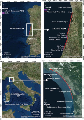
The Atlantic Study Area (ASA, Figure 1 – first row) is located between the municipalities of Ovar and Marinha Grande on the northwest Portuguese mainland coast. It is a wide coastal plain, ca. 140 km long, made up almost exclusively of sandy beaches landward bordered by dune systems. Dunes are generally covered by vegetation even though they are locally disrupted by urban settlements. Shoreline continuity is interrupted by the Ria de Aveiro lagoon with its artificial port, the cliff of Serra da Boa Viagem (located to the north of the Figueira da Foz Port and the Mondego estuary), and the cliff of São Pedro de Moel. The typical beach profile is characterized by three features: sandy beach; seaward dune area, covered by scattered vegetation; and inward stable dune area, covered by dense and stable vegetation. The wave regime is mainly northwest oriented with 2 m mean wave height and 12 s mean wave period. The tidal regime is semi-diurnal with a spring tidal range between 2 and 4 m. Longshore currents, mainly generated by wave action, are southward and the area is affected by severe erosive processes, mainly due to sea action and reduced sediment supply from the Douro River. In order to mitigate erosion, several coastal protection measures, e.g., groins and seawalls, have been built (Silva et al. 2009; Roebeling, Coelho, and Reis 2011; Baptista et al. 2014). In the ASA, a new generation of coastal spatial and management plans (Table 1), redefined as special regional programs, have been implemented (approved by the Decree-Law no. 80/2015). In Portugal, they represent the first example of plans implementing buffer zones against coastal erosion, sea-wave overtopping, and coastal flooding. They represent a practical tool to apply risk management principles to decrease the vulnerability of (new) urban settlements in hazard-prone areas. The first steps of the planning process include the characterization and prospective diagnosis followed by development of the plan proposal (Alves et al. 2014), during which GbSAM was implemented to assess past ASA shoreline changes and obtain a quantitatively based predictive scenario from which erosion-prone areas were defined (Cenci et al. 2013).

Table 1. Main strategic and operational documents on the Atlantic Study Area (ASA) and the Mediterranean Study Area (MSA).

	ASA	MSA
Main strategic and operational documents	Coastal zone program for Ovar–Marinha Grande (2016–2027)^a	Two regional spatial plans: Liguria^b and Tuscany^c regions
Spatial scale	500 m buffer from the shoreline (up to 1000 m)	Spatial plan binding within a buffer of 300 m from the shoreline^d
Risk management principles	Safeguard zones for coastal erosion, wave overtopping, and coastal flooding Lower level of risk:● No further fixed-building constructions beyond existing urban limits● The construction of new buildings inside urban limits must fulfill specific accommodation/adaptation requirementsHigher level of risk:● All new constructions are forbidden● Increased limitations for reconstructions/reconfiguration of existing buildings● Planned demolitions and re-naturalization in degraded areas	Landscape plan binding and conditioned land-use apply within 300 m from the shoreline Bindings do not apply if the hydraulic safety and sediment transport flow is ensured^c

ASA: Atlantic Study Area; MSA: Mediterranean Study Area.

^aPrograma para a Orla Costeira Ovar–Marinha Grande (redefined as a territorial management instrument by the Decree-Law no. 80/2015, of May 14; under public discussion in December 21, 2015).

^bRegional law 39/1984: Piano territoriale di coordinamento paesistico, Piano territoriale di coordinamento della costa.

^cRegional Council Resolution 37/2015: Piano di indirizzo territoriale della Regione Toscana con valenza di piano paesaggistico.

^dIntroduced by Decree-Law 431/1985 and reinforced by Decree-Law 42/2004 and Decree-Law 157/2006.

Figure 1. Study Areas. Atlantic Study Area (ASA), upper row. Mediterranean Study Area (MSA), bottom row.

2.2. Mediterranean Study Area

The Mediterranean Study Area (MSA, Figure 1 – second row) is located between the Magra and Serchio river mouths along the northwest Italian coast. It is ca. 40 km long coastal stretch mainly comprising sandy beaches. The northern sector consists of mixed sand and gravel and except for the southern part, most of the study area is urbanized. Shoreline continuity is interrupted by the Marina di Carrara and Viareggio Ports. Wave height and period are estimated to be 7.54 m and 9.15 s, respectively, with a microtidal regime and an astronomical tidal range of 0.35 m. Principal rivers contributing to sediment supply are the Arno and Magra, with the Serchio River making a minor contribution. Over the past century, river sediment supply has decreased because of in-river works and land use changes, and consequently from the Magra River to Marina di Massa, coastal defense structures have been built (Pranzini and Farrell 2004; Anfuso, Pranzini, and Vitale 2011). Within the MSA, new construction is forbidden within a 300-m buffer from the shoreline, in accordance with regional spatial plans of the Liguria and Tuscany regions (Table 1) and following the principles of the “Galasso Act” (D.L. 431/1985).

3. Method

3.1. Data source: the Landsat archive

The dataset comprised optical images of the Landsat archive acquired by the Thematic Mapper (TM), Enhanced Thematic Mapper Plus (ETM+) and Operational Land Imagery (OLI) sensors. Images have a spatial resolution of 30 m in VISible, Near Infra-Red (NIR) and Short Wave Infra-Red (SWIR) bands. ASA dataset included images from 1984, 1987, 2000, 2003, 2007, 2009, 2011, and 2014, while the MSA dataset included images from 1987, 1990, 2001, 2004, 2009, 2011, and 2014. A single image per year was selected, as the implemented model assumes that any shoreline (or its proxy) is an instantaneous “snapshot” of its dynamic position in time and affected by some random component (i.e., noise). In order to use images that were free from cloud cover, analyses were undertaken for the following periods: 24 June–15 October (ASA) and 7 April–18 September (MSA). Furthermore, choosing these time periods enabled mitigation of seasonal influences on proxy extraction and was found to be the best trade-off between data availability and climatic constraints.

3.2. Proxies definition

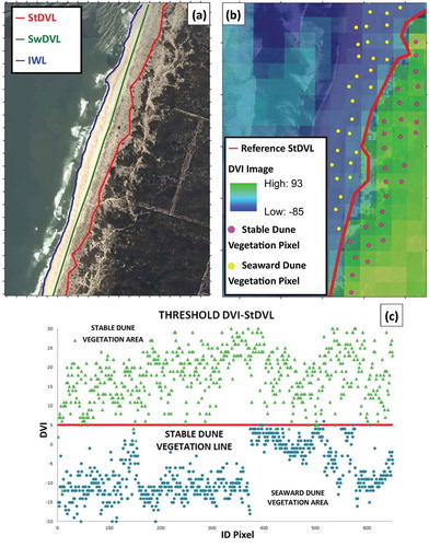
The “original” proxy chosen to implement the GbSAM in ASA was the StDVL (Cenci et al. 2013). This was defined as the line separating the dune area which is mainly covered by dense and stable vegetation, from the seaward area that is mainly occupied by scattered vegetation (Thomas et al. 2011). In the ASA, the GbSAM was also applied to other proxies such as the SwDVL, seen as the line dividing the seaward, scattered vegetation from the beach area without vegetation, and the IWL, i.e., the position of the beach–sea boundary at an instant in time (Boak and Turner 2005). The three proxies (Figure 2(a)) were used for carrying out the multi-proxy analysis. For the MSA, strong anthropic beach pressures resulted in destruction of the natural continuity of the dune system in nearly all assessed areas, and consequently only the IWL proxy was used.

Figure 2. In Figure 2(a) are represented the three proxies used in this paper (as example, in the picture, it is shown an exemplifying coastal stretch belonging to the ASA). In Figure 2(b), it is shown the sampling of the 2011 DVI image pixels’ values in the stable dune vegetation/seaward dune vegetation transitional area. In Figure 2(c), it is shown the definition of the DVI value representative of the StDVL threshold (i.e., the median of the whole statistical population of the sampled pixels).

3.3. Geomatic-based shoreline analysis method (GbSAM)

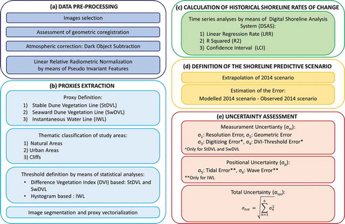
GbSAM consists of five stages: (A) data preprocessing, (B) proxy extraction, (C) calculation of historical shoreline rates of change, (D) definition of the shoreline predictive scenario, and (E) uncertainty assessment.

3.3.1. Data preprocessing

A preprocessing step was needed to obtain a multi-temporal dataset that was geometrically and radio-metrically co-registered. This is the fundamental prerequisite to accurately extract coherent proxies in space and time. Landsat images were downloaded as Level 1T product (Standard Terrain Correction) and georeferenced to the Universal Transverse Mercator map projection system (ASA: zone 29 N, Path: 204, Row: 32; MSA: zone 32 N, Path: 193, Row: 29). Images were provided with metadata, which includes residuals of ground control points used to perform orthorectification. The quality of spatial co-registration among images belonging to the same dataset was checked by means of the geometric root mean square error (RMSE) model (USGS 2016). Within the datasets, the maximum of the geometric RMSE model values were 4.5 and 6.8 m for ASA and MSA, respectively. Given Landsat spatial resolution, these values were considered adequate, i.e., smaller than half the pixel size and therefore, no further image spatial co-registration was carried out. With respect to image radiometry, top of atmosphere radiance was calculated from digital numbers by adopting the coefficients and equations reported in Chander, Markham, and Helder (2009). Landsat 8 images were converted by exploiting the ENVI tool “Radiometric Calibration” (ENVI 2016) and subsequently a two-step radiometric correction was performed. First, effects of atmospheric scattering were mitigated by applying the dark object subtraction method (Song et al. 2001). Residual radiometric mis-registration amongst images was reduced by applying a linear relative radiometric normalization (Yuan and Elvidge 1996; Yang and Lo 2000) based on pseudo invariant features (PIFs) (Schott, Salvaggio, and Volchok 1988) selected in all images of both study areas. PIFs were visually selected in relatively flat areas, approximately located at the same elevation. This is so that atmospheric thickness over each target was almost the same and the sun angle between images did not produce different effects. Furthermore, they were chosen to provide a wide range of radiance values, to obtain a reliable regression model (Eckhardt, Verdin, and Lyford 1990).

3.3.2. Proxy extraction

Before extracting proxies, study areas were classified into three thematic classes, i.e., natural areas, urban areas, and cliffs, by visual interpretation of the high-resolution base map provided in ESRI ArcGIS software. Criteria adopted for these classifications were natural areas are coastal stretches of beach where shoreline evolution is assumed to be dominated by “natural” processes without direct anthropic influences and urban areas are beach sections close to urban coastal settlements, where protection structures such as groins and revetments may directly/strongly influence coastal processes. In ASA, all beaches located in front of urban settlements were classified as urban areas, whereas in MSA, the coastline from Magra River to Marina di Massa was classified as such. Analyses were not performed along coastal cliffs, located within ASA only, because in these areas, coastline change processes follow different dynamics with respect to sandy shores. In ASA, urban areas were excluded from assessments based on StDVL and SwDVL, hereinafter also defined as vegetation-based proxies, because dune vegetation was destroyed and replaced by urban structures.

With respect to vegetation-based proxies, their extraction was achieved by exploiting auxiliary, high-resolution, reference data: natural color digital orthophotos, dated 2011, with a spatial resolution of 0.5 m, were available for the whole ASA shoreline (National Environment Agency, formerly INAG I.P). The StDVL was visually identified on the 2011 orthophotos, with the delineation process repeated several times to enable uncertainty related to visual interpretation, namely the Digitizing Error, to be estimated (see Section 3.3.5). The final orthophotos-based reference line was obtained as the median of the visually delineated lines. Subsequently, the difference vegetation index (DVI = NIR–Red) (Lillesand and Kiefer 1987) was calculated by using 2011 Landsat image. Subsequently, DVI threshold values provided the best representation of the proxy previously delineated on the orthophotos. To this end, the same number of pixels belonging to the stable dune vegetation/seaward dune vegetation (seaward dune vegetation/beach in the SwDVL case) was sampled in transitional areas on the 2011 DVI Landsat image, by applying a bilinear interpolation algorithm. Then, threshold values were chosen as the median of the sampled global statistical population (Figure 2(b,c)). After proxy vectorization, visual editing allowed to identify and remove local misclassification errors. Since image datasets were previously radiometrically co-registered, the threshold value was used to classify and extract the vegetation-based proxies from all images in the ASA dataset.

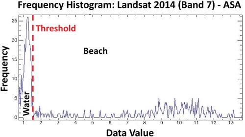
The IWL proxy was successfully extracted in both natural and urban study areas. Since this proxy is extremely dynamic due to combined effects of tidal cycles, wind, sea waves and energy, and atmospheric pressure, auxiliary high-resolution data could not be used as a reference when extracting this proxy. Therefore, a different procedure was implemented based on the consideration that in the SWIR region of the electromagnetic spectrum, water absorbs almost all the solar radiation, whereas land is characterized by higher values of radiance (or reflectance). Consequently, a conventional method of detecting the land/water boundary may consist of a SWIR band thresholding (White and El Asmar 1999; Paul Shane and John Page 2000; Cenci et al. 2017). This approach was used to extract the IWL from every SWIR band (band number 7) of the images. The threshold value was chosen by sampling the same number of pixels classified as “beach” and “water” in different training sites of the transitional area and by analyzing their frequency histogram to find the corresponding value of an abrupt spectral change (Figure 3). This value was defined for reference images from both study areas and subsequently applied to the whole multi-temporal dataset.

Figure 3. Frequency histogram of the ASA 2014 Landsat image, band 7. The threshold value corresponding to an abrupt spectral change is represented in red.

3.3.3. Calculation of historical shoreline rates of change

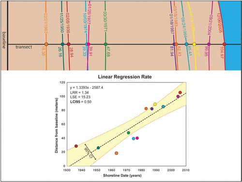
The time series of shoreline positions represented by proxy vector data was used to calculate rates of change along equally spaced (100 m) transects casted perpendicularly to the shore by means of the Digital Shoreline Analysis System (DSAS), a freely available application that works within the ESRI ArcGIS software (Thieler et al. 2008). DSAS allowed the calculation, for all transects, of the linear regression rate (LRR), representative of the proxy annual displacement rate (m/year). For each transect, the LRR was calculated as the slope of the least-squares regression line of the shorelines’ position (Figure 4). DSAS provided also, for each transect, (1) the coefficient of determination (R-squared – R²) and (2) the uncertainty associated to every LRR, calculated as the 95.5% confidence interval (LCI) of the reported rate.

Figure 4. Schematic representation of the LRR, R², and LCI calculation. Source: Adapted from Thieler et al. (2008).

3.3.4. Definition of the shoreline predictive scenario

LRR values were used to predict the 2014 scenario by assuming, for the short time period of the extrapolation, a constant annual rate of change (i.e., LRR). Therefore, modifications to sediment transport dynamics and climate change effects, including sea level rise, were neglected.

3.3.5. Uncertainty assessment

Several sources of uncertainty affect historical shoreline mapping and, in turn, shoreline rates of change. Fletcher et al. (2003) grouped them in two categories: measurement uncertainty (σ_m) and positional uncertainty (σ_p), where σ_m is related to operator-based data processing and data source/s characteristics (e.g., pixel size, orthorectification, visual delineation process) and σ_p is related to factors influencing the definition of the real shoreline position during a given year (e.g., tides, storms, seasonal state of the beach). These uncertainties are assumed to be random, not correlated and quantified in a global estimation (σ_tot) by calculating the square root of the sum of the squares of all uncertainty factors, σ_n (Fletcher et al. 2003) (Table 2). In this study, the factors determining σ_m were resolution error (σ₁), geometric error (σ₂), digitizing error (σ₃), and DVI-threshold error (σ₄). The digitizing error and the DVI-threshold error affected only vegetation-based proxies. Given the similarities between the Landsat’s sensors, uncertainty due to their different spectral and radiometric resolutions was considered negligible. Factors determining σ_p were tidal error (σ₅) and wave error (σ₆). These factors affected only the estimation of the IWL. When extracting the StDVL and the SwDVL, seasonal effects of the phenological cycle on vegetation were considered negligible. For all the proxies, climate change effects were also neglected. The resolution error was set equal to image pixel size, because theoretically it is not possible to resolve features smaller than this value (Virdis, Oggiano, and Disperati 2012). Geometric error was assumed to be representative of the geometric error of the orthorectification process and it was calculated as the mean of the geometric RMSE model values reported in the images metadata. Digitizing error was evaluated by delineating several times the vegetation-based proxies on the orthophotos and calculating the error as the standard deviation of position residuals for that feature (Virdis, Oggiano, and Disperati 2012). DVI-threshold error was assumed to be equal to the residuals between the StDVL and SwDVL reference lines mapped from the orthophotos and the ones extracted from the 2011 Landsat image. Because of different tidal condition among the study areas, tidal error was calculated as the projection of the mean tidal range (ASA: 3 m; MSA: 0.35 m) on the shore, as defined by Bird (2008). Shore mean slope values (ASA: 5°; MSA: 3.7°) were estimated from LIDAR data (2 m spatial resolution) available for both study areas, from which shorelines were visually mapped. LIDAR slope statistics were assumed to be representative for the whole time span under consideration (Virdis, Oggiano, and Disperati 2012). Wave error was assumed equal to the projection of the mean summer wave height [ASA: 1.5 m (MAMAOT/APA, I.P 2012); MSA: 0.67 m – measured at La Spezia buoy in the time interval 1989–2007] on the shore, according to their mean slope values. Final uncertainty values are reported in Table 2.

Table 2. Uncertainty assessment.

	Uncertainty factors ()	StDVL (ASA)	SwDVL (ASA)	IWL (ASA)	IWL (MSA)
Measurement uncertainty () (m)	Resolution error ()	30	30	30	30
	Geometric error ()	4	4	4	4
	Digitizing error ()	5	5	0	0
	DVI-threshold error ()	12	9	0	0
Positional uncertainty () (m)	Tidal error ()	0	0	34	5
	Wave error ()	0	0	17	10
Total uncertainty () (m)		±33	±32	±49	±32

StDVL: Stable dune vegetation line; IWL: instantaneous water line; ASA: Atlantic Study Area; MSA: Mediterranean Study Area.

A value equal to 0 m was set for the uncertainty factors that were not used in the computation of σ_tot of each proxy.

It is worth noting that in analyses, the not-weighted linear regression (WLR) approach (i.e., LRR and LCI) was used because (1) the resolution error was constant in both datasets and (2) the geometric error was considered constant within each dataset, because standard deviations of the mean geometric RMSE model values (ASA: 1 m; MSA: 1.4 m) can be considered negligible with respect to spatial resolution of the Landsat archive. If these conditions are not met (e.g., the standard deviation is higher and thus no longer negligible, or if different satellite images with different spatial resolutions are used), the WLR and the confidence interval of WLR (WCI) should be used in DSAS to calculate historical rates of change and evaluate uncertainty (Thieler et al. 2008).

A detailed graphical description of the GbSAM stages is provided in Figure 5.

Figure 5. Description of the GbSAM stages.

4. Results and discussion

Results are reported in Table 3 and Figures 6–8. In Figures 6(a–c) and 7(a), LRR and R² values of each transect for all proxies are shown for ASA and MSA, respectively. LRR graphs describe the different evolution trends for the study areas, allowing identification and quantification of shoreline retreat (negative values) and advancement (positive values). Figure 8 shows the model uncertainty (LCI values) associated with each proxy, while Table 3 reports statistics determined to evaluate proxy performances. Further details are provided as follows.

Table 3. Summary statistics of the statistical analyses carried out in Section 4.

	StDVL (ASA)	SwDVL (ASA)	IWL (ASA)	IWL (MSA)
Percentage of transects SNR > 1 (%)	90	92	77	59
R^2 mean values (and standard deviations) (−)	0.72 (0.2)	0.38 (0.3)	0.52 (0.3)	0.53 (0.3)
LCI mean values (and standard deviations) (m/year)	±1.9 (1.6)	±3.2 (1.9)	±1.9 (1)	±1.2 (0.7)
Mean absolute error (m)	16.7	49.5	22	8.3
Mean error (m)	1.1	49	−14.6	1.1
Error standard deviation (m)	23.7	34.6	17.9	7.4
Root mean squared error (m)	29	60.3	28.4	11.1

StDVL: Stable dune vegetation line; SNR: signal-to-noise ratio; IWL: instantaneous water line; ASA: Atlantic Study Area; MSA: Mediterranean Study Area.

Figure 6. The figure shows the LRR, R², and error results obtained for the proxies of the ASA (StDVL, SwDVL, and IWL). In all the graphs, on the X-axes is reported the position of transects expressed as distance from the first transect that was casted at the beginning of the study area in Ovar and proceeding toward south. In the StDVL and SwDVL diagrams, X-axes start from ca. −3000 because there is a shift of ca. 3 km with respect to the IWL because of the occurrence of an urban areas (close to the Ovar town) that is taken into account only for the IWL analysis. The shifting is necessary to graphically homogenize all ASA graphs.

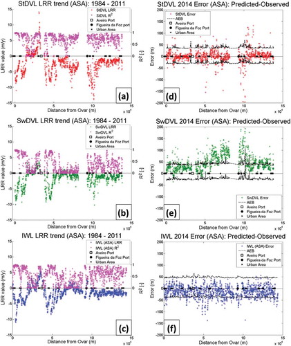
Figure 7. The figure shows the LRR, R², and error results obtained for the proxy of the MSA (IWL). On the X-axes is reported the position of transects expressed as distance from the first transect that was casted at the beginning of the study area (Magra River Mouth) and proceeding toward south.

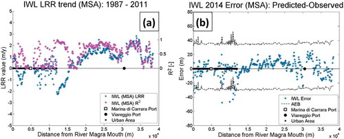
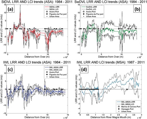
Figure 8. The figure shows the different uncertainty, in terms of LCI, associated to the LRR of each proxy’s transect. In order to reduce the noise, and thus increase graphs readability, LRR and LCI data were smoothened by applying a moving average filter (span equal to 5; i.e., 500 m) and plotted as continuous lines. Therefore, in the graphs are present some artifacts (i.e., presence of data in areas excluded from the elaborations, such as urban areas).

4.1. Atlantic study area

Before analyzing ASA results, a preliminary assessment to evaluate uncertainty of Landsat-based proxies was undertaken. The ratio between the shoreline change envelope (SCE) and σ_tot of each proxy was chosen as an expression of the signal-to-noise ratio (SNR). SNR was used to statistically evaluate if the Landsat archive is an adequate tool to measure ASA shoreline evolution. The SCE is a statistical output provided by DSAS that represents, for each transect, the total shoreline movement for all available shoreline positions, expressed in absolute values without temporal consideration (Thieler et al. 2008). For transects with SNR > 1, the shoreline displacement signal can theoretically be detected by the analysis. For each proxy, the percentage of transects with SNR > 1 is reported in Table 3.

For ASA, it is worth noting that GbSAM allowed a multi-proxy analysis of shoreline evolution. This analysis showed a general tendency of shoreline retreat for all proxies, a finding which also agrees with other studies (Taveira-Pinto, Silva, and Pais-Barbosa 2011; Lira et al. 2016). Such agreement is a remarkable result because the comparison of rates obtained by using different proxies is not obvious, since their evolution can be affected by different processes, with different spatial and temporal scales. All proxies detected shoreline advance in areas to the north of the Port of Aveiro, where infrastructure allows deposition of sediment carried by longshore currents. Other positive rates can be observed in both SwDVL and IWL graphs, but not by StDVL (Figure 6). Such differences should be analyzed carefully using in situ observations and measurements. A small-scale analysis based on field observations was not undertaken as it is beyond the scope of this work that is aimed at providing information at regional and subregional level. Differences between proxy trends can be useful for deeper understanding of the complex processes acting on a given littoral. Since evolution of different proxies can be affected by different factors, in addition to those strictly related to shoreline dynamics, multi-proxy analyses can highlight such differences. For example, an analysis based on vegetation-based proxies can provide useful information about changes in vegetation dynamics but partially contradicts assumptions underpinning any shoreline analysis based on proxy trends. However, it is argued that this limitation is still important for coastal risk assessment and ICM and that a multi-proxy analysis can help in defining areas where results are more reliable, i.e., where all proxies show similar results (such as north of the Port of Aveiro), and areas where there is a disagreement between proxy trends. The latter can be the objective of different kinds of analyses (e.g., small scale based on field observations) with different aims (e.g., vegetation dynamics in studies using vegetation-based proxies).

Trend analysis was integrated by evaluations of R² (Figure 6(a–c)) and LCI (Figure 8(a–c)). Spatial representation of R² values is shown in Figure 6(a–c), while mean R² values and standard deviations are given in Table 3. StDVL is the proxy that better fits assumptions of linearity intrinsic to the adopted linear model (Figure 6(a)) and is likely to be less affected by seasonal or daily fluctuations (i.e., noise) when compared to SwDVL and IWL. Therefore, it may be more suitable to describe longer term changes using a linear model. Instead, nonlinear models may be necessary for describing the evolution of other proxies and/or shorter term trends. Mean LCI values and their standard deviations are shown in Table 3. Since the StDVL signal (i.e., LRR values) was highest, mean LCI value suggests that uncertainty affecting modeling of this proxy is lower than for other proxies. Figure 8(b) also shows that SwDVL is the proxy affected by highest model uncertainty.

Prediction accuracy was assessed by comparing modeled scenarios with observed proxies extracted from 2014 images. The error, defined as the difference between modeled and observed proxy positions, was determined for each transect, and the following statistics were subsequently calculated: mean absolute error, mean error, error standard deviation, and RMSE (Table 3). Spatial representation of error is shown in Figure 6(d–f), where positive values represent an overestimation of predicted displacement with respect to that observed. The graphs also show for each proxy, the upper and lower admissible error boundaries (AEB), defined as AEB = σ_tot ± 3 × LCI. These boundaries take into account uncertainty of the 2014 proxy and of the 2014 predicted scenario. A 2014 prediction with an error value included in the range ±AEB is considered reliable. Overall, the analysis of the 2014 scenario again highlighted the better performance of StDVL with respect to the other proxies. Higher values of SwDVL and IWL error statistics suggest that future predictions may lack accuracy if a linear model, set up to capture long-term trends, is applied for short-term predictions of “less stable” coastal features that are used as proxies. With respect to IWL, the greater number of predictions with an Error value included in the range ±AEB is a consequence of the higher σ_tot value associated to this proxy.

Therefore, it is argued that StDVL is the more reliable proxy to study ASA shoreline evolution by means of GbSAM. This proxy has been already used in earlier phases of the coastal zone program (Table 1) to identify changes in rates of shoreline advance or retreat and areas prone to risk. SwDVL appears to be the less reliable proxy to be used with a linear model. IWL, despite not being particularly suitable for a linear model and affected by high degree of uncertainty (σ_tot), is the only one that allows analysis of urban areas. Consequently, IWL-based analyses may be particularly useful for ICM, in particular where municipal spatial plans apply (in which coastal zone programs become strategic and nonoperational). Due to the concentration of assets at stake, these areas are more vulnerable and therefore more exposed to coastal hazards and risk. If in urban areas it is difficult to model shoreline evolution because of strong anthropic influences on coastal processes, which are likely to affect long-term model statistics, IWL-based analyses can provide a valuable monitoring tool, especially following a significant event such as storm or coastal flood, i.e., near real-time shoreline monitoring, rapid shoreline change assessment, etc.

4.2. Mediterranean study area

For MSA, LRR values (Figure 7(a)) clearly define areas characterized by retreat or advance and quantify all these processes. Retreat is observed in the northern part from the Magra River to Marina di Massa, an area previously classified as urban areas, whereas advance is recognized in the southern part. Comparison with results obtained by other authors such as Pranzini and Farrell (2004) and Anfuso, Pranzini, and Vitale (2011) is no trivial task because different trends can be obtained for the same coastline by adopting different data sources, proxies, methods, and/or time intervals (Taveira-Pinto, Silva, and Pais-Barbosa 2011). However, patterns can be considered similar. Statistical scores determined for ASA were also calculated for MSA with results related to characterization of shoreline evolution trends shown in Table 3.

The low percentage of transects with SNR > 1 can be explained by the moderate spatial resolution of Landsat images in microtidal environments such as MSA. Furthermore, adoption of IWL as proxy implies a higher degree of uncertainty due to influences of tidal and wave errors. Nevertheless, the linear model allowed long-term trends to be resolved from random fluctuations due to tidal and wave effects and produced trends similar to those obtained in other studies such as Pranzini and Farrell (2004) and Anfuso, Pranzini, and Vitale (2011). R² values are lower for urban areas (Figure 7(a)), where erosive processes are known and engineering structures have been built to protect the littoral. Conversely, R² values are higher where the coast was classified as a natural area, suggesting that linear models are more suitable for natural rather than urban areas. Earlier considerations regarding IWL analyses in urban areas are valid. Statistics related to the accuracy assessment of the future 2014 scenario are shown in Table 3. These statistics are again influenced by moderate spatial resolution of the Landsat archive, as well as fluctuations such as tidal error and wave error that may reduce the reliability of short-term predictions based on long-term rates. The graph “IWL 2014 Error (MSA): Predicted-Observed” (Figure 7(b)) shows how high values of σ_tot produce wider AEB. This means that predictions can be considered accurate but only relative to the high degree of uncertainty associated with the IWL proxy. The graph “IWL LRR and LCI Trends (MSA): 1987–2011” (Figure 8(d)) shows that given the signal recorded, there is high model uncertainty associated with IWL.

Finally, it is argued that for ICM and coastal risk reduction, the implementation of GbSAM in MSA has some drawbacks caused by Landsat spatial resolution and adoption of IWL as proxy. However, in the absence of other proxies and satellite data, GbSAM produced valuable information to infer consequences of coastal processes that could be acting in the MSA littoral. Based on changes and trends expected for MSA, this information will be useful to support judgments linked to applications for exceptions within the 300-m buffer (Table 1). Further improvements are expected if in the future, other satellite data (not only optical) with higher spatial resolutions (e.g., Sentinel 1, Sentinel 2) are used to decrease σ_tot (Cenci et al., “Remote Sensing for Coastal Risk Reduction Purposes”: Cenci et al. 2015a) and detect processes that are characterized by lower signals with higher accuracy.

5. Conclusions

This paper presented an improved version of a simple, robust, and repeatable method, GbSAM (Cenci et al. 2013), to integrate remote sensing and GIS techniques for mapping positions of shoreline proxies and modeling their evolution over time. The aim was to describe an end-to-end processing chain of satellite data to define past, present, and future areas prone to shoreline erosion, at regional and subregional level and support coastal risk management. The Landsat archive was used as input data, but the method can be easily applied with other satellite data. GbSAM enabled accurate and consistent extraction of shoreline proxies that were coherent in space and time. These proxies were subsequently used to calculate historical shoreline rates of advance/retreat using a linear model that also allowed extrapolating future scenarios. The latter were validated by comparing the modeled 2014 scenario with that observed, with results statistically analyzed and interpreted within a coastal risk management framework. Analysis focused on two different study areas to test GbSAM capabilities in different coastal environments: Atlantic – ASA (high energy) and Mediterranean – MSA (low energy). Findings showed:

• The method provided valid results, proven to be more accurate where the coast is not urbanized (i.e., natural areas) and when the shoreline change signal is larger (i.e., ASA). Considerable improvements are expected, especially in MSA-like environments, if/when long and continuous time series of observations obtained by satellite sensors at higher spatial resolution is used to decrease the geometric error (which in turn highly affects the method uncertainty, σ_tot).

• The multi-proxy analysis approach is important for a deeper understanding of coastal process acting on a given littoral and for defining which proxy is more reliable in a given study area. Results showed that proxies based on stable coastal features (e.g., StDVL) produce more accurate results because they have a lower degree of uncertainty and are less affected by daily/seasonal fluctuations.

• When predicting short-term scenarios based on long-term advance/retreat rates, extrapolation obtained from stable coastal features is more accurate.

To conclude, this research has shown that by using the Landsat archive, GbSAM can contribute to achieve ICM objectives by defining which areas are more susceptible to present and future coastal hazards and risk, especially in ASA-like environments.

Acknowledgments

Luca Cenci is grateful to Simone Cenci for the endless and fruitful discussions. The authors are also grateful to the anonymous four reviewers.

Disclosure statement

No potential conflict of interest was reported by the authors.

Additional information

Funding

Part of this study was supported by the FCT/MEC national funding to CESAM: [Grant Number UID/AMB/50017/2013] and by FEDER co-funding within the PT2020 Partnership Agreement and Compete 2020. The PhD grant SFRH/BD/104663/2014 (E.R. Oliveira) is also acknowledged.

References

- Alves, F. L., L. P. Sousa, T. C. Esteves, E. R. Oliveira, I. C. Antunes, M. D. L. Fernandes, L. Carvalho, S. Barroso, and M. Pereira. 2014. “Trend Change(S) in Coastal Management Plans: The Integration of Short and Medium Term Perspectives in the Spatial Planning Process.” Proceedings 13th International Coastal Symposium (Durban, South Africa), Journal of Coastal Research, Special Issue, no. 70: 437–442. doi:10.2112/SI70-074.1.
- Anfuso, G., E. Pranzini, and G. Vitale. 2011. “An Integrated Approach to Coastal Erosion Problems in Northern Tuscany (Italy): Littoral Morphological Evolution and Cell Distribution.” Geomorphology 129 (3–4): 204–214. Elsevier B.V. doi:10.1016/j.geomorph.2011.01.023.cenci
- Baptista, P., C. Coelho, C. Pereira, C. Bernardes, and F. Veloso-Gomes. 2014. “Beach Morphology and Shoreline Evolution: Monitoring and Modelling Medium-Term Responses (Portuguese NW Coast Study Site).” Coastal Engineering 84 : 23–37. Elsevier B.V. doi:10.1016/j.coastaleng.2013.11.002.
- Bird, E. 2008. Coastal Geomorphology. An Introduction. John Wiley & Sons. doi:10.1007/s13398-014-0173-7.2.
- Boak, E. H., and I. L. Turner. 2005. “Shoreline Definition and Detection: A Review.” Journal of Coastal Research 21 (4): 688–703. doi:10.2112/03-0071.1.
- Cenci, L. 2013a. GIS and Remote Sensing for Coastal Evolution Studies: Multi-Proxy Shoreline Changes in the Ovar–Marinha Grande Area (Portugal) from 1984-2011 and 2022 Scenarios. Italy: University of Siena.
- Cenci, L. 2013b. “L ’ Importanza Della Scelta Del Proxy E Del Fattore ‘ Incertezza ’ Nel Monitoraggio Dell ’ Evoluzione Costiera Tramite Dati Telerilevati.” In Atti 17a Conferenza Nazionale ASITA 2013, 427–434. Riva del Garda 5-7 novembre 2013. http://atti.asita.it/ASITA2013/Pdf/188.pdf
- Cenci, L., G. Boni, L. Pulvirenti, G. Squicciarino, S. Gabellani, F. Gardella, N. Pierdicca, and M. Chini. 2017. “Monitoring Reservoirs’ Water Level from Space for Flood Control Applications. A Case Study in the Italian Alpine Region.” 2017 IEEE International Geoscience and Remote Sensing Symposium (IGARSS), Fort Worth, 5617–5620.
- Cenci, L., L. Disperati, L. P. Sousa, M. Phillips, and F. L. Alves. 2013. “Geomatics for Integrated Coastal Zone Management: Multitemporal Shoreline Analysis and Future Regional Perspective for the Portuguese Central Region.” Proceedings 12th International Coastal Symposium (Plymouth, England), Journal of Coastal Research, Special Issue No. 65, 1349–1354. doi:10.2112/SI65-228.1.
- Cenci, L., M. G. Persichillo, L. Disperati, E. R. Oliveira, F. L. Alves, L. Pulvirenti, N. Rebora, G. Boni, and M. Phillips. 2015a. “Remote Sensing for Coastal Risk Reduction Purposes: Optical and Microwave Data Fusion for Shoreline Evolution Monitoring and Modelling.” 2015 IEEE International Geoscience and Remote Sensing Symposium (IGARSS), Milan, 1417–1420. doi:10.1109/IGARSS.2015.7326043.
- Cenci, L., M. G. Persichillo, L. Disperati, E. R. Oliveira, F. L. Alves, G. Boni, L. Pulvirenti, and M. Phillips. 2015b. “Validation of a Short-Term Shoreline Evolution Model and Coastal Risk Management Implications. The Case of the NW Portuguese Coast (Ovar-Marinha Grande).” In EGU General Assembly 2015, 6299. Vol. 17.Vienna: Geophysical Research Abstracts.
- Chander, G., B. L. Markham, and D. L. Helder. 2009. “Summary of Current Radiometric Calibration Coefficients for Landsat MSS, TM, ETM+, and EO-1 ALI Sensors.” Remote Sensing of Environment 113 (5): 893–903. Elsevier Inc. doi:10.1016/j.rse.2009.01.007.
- Crowell, M., B. C. Douglas, and S. P. Leatherman. 1997. “On Forecasting Future U.S. Shoreline Positions: A Test of Algorithms.” Journal of Coastal Research 13 (4): 1245–1255.
- Crowell, M., S. P. Leatherman, and M. K. Buckley. 1993. “Shoreline Change Rate Analysis: Long Term Versus Short Term Data.” Shore and Beach 61 (2): 13–20.
- Douglas, B. C., M. Crowell, and S. P. Leatherman. 1998. “Considerations for Shoreline Position Prediction.” Journal of Coastal Research 14 (3): 1025–1033.
- Douglass, S. L., T. A. Sanchez, and S. Jenkins. 1999. “Mapping Erosion Hazard Areas in Baldwin County, Alabama and the Use of Confidence Intervals in Shoreline Change Analysis.” Journal of Coastal Research, no. Special Issue No 28: 95–105.
- EC. 2016. “Iczm.” http://ec.europa.eu/environment/iczm/home.htm.
- Eckhardt, D. W., J. P. Verdin, and G. R. Lyford. 1990. “Automated Update of an Irrigated Lands GIS Using SOPT HRV Imagery.” Photogrammetric Engineering and Remote Sensing 56 (11): 1515–1522.
- ENVI. 2016. “Radiometric Calibration.” http://www.harrisgeospatial.com/docs/RadiometricCalibration.html.
- Fenster, M. S., R. Dolant, and J. F. Elder. 1993. “A New Method for Predicting Shoreline Positions from Historical Data.” Journal of Coastal Research 9 (1): 147–171.
- Ferreira, Ó., T. Garcia, A. Matias, R. Taborda, and J. Alveirinho Dias. 2006. “An Integrated Method for the Determination of Set-Back Lines for Coastal Erosion Hazards on Sandy Shores.” Continental Shelf Research 26 (9): 1030–1044. doi:10.1016/j.csr.2005.12.016.
- Fletcher, C., J. Rooney, M. Barbee, S. C. Lim, and B. Richmond. 2003. “Mapping Shoreline Change Using Digital Orthophotogrammetry on Maui, Hawaii.” Journal of Coastal Research, Special Issue No. 38: 106–124.
- Li, W., and P. Gong. 2016. “Continuous Monitoring of Coastline Dynamics in Western Florida with a 30-Year Time Series of Landsat Imagery.” Remote Sensing of Environment 179 : 196–209. Elsevier Inc.:. doi:10.1016/j.rse.2016.03.031.
- Lillesand, T. M., and R. W. Kiefer. 1987. Remote Sensing and Image Interpretation. 2nd ed. John Wiley and Sons.
- Lira, C., P. Ana Nobre Silva, R. Taborda, and C. Freire De Andrade. 2016. “Coastline Evolution of Portuguese Low-Lying Sandy Coast in the Last 50 Years: An Integrated Approach.” Earth System Science Data 8: 265–278. doi:10.5194/essd-8-265-2016.
- MAMAOT/APA, I.P. 2012. POOC Ovar-Marinha Grande: Volume I. Relatório: Caracterização E Diagnóstico Prospectivo. Lisbon (Portugal).
- Milli, M., and L. Surace. 2011. Le Linee Della Costa: Definizioni, Riferimenti Altimetrici E Modalit{À} Di Acquisizione Dei Dati. Alinea. https://books.google.it/books?id=KitrXxcRKPEC.
- Morton, R. A., T. L. Miller, and L. J. Moore. 2004. “National Assessment of Shoreline Change: Part 1: Historical Shoreline Changes and Associated Coastal Land Loss along the US Gulf of Mexico.” U.S. Geological Survey Open-File Report 2004-1043, 45.
- Mukhopadhyay, A., S. Mukherjee, S. Mukherjee, S. Ghosh, S. Hazra, and D. Mitra. 2012. “Automatic Shoreline Detection and Future Prediction: A Case Study on Puri Coast, Bay of Bengal, India.” European Journal of Remote Sensing 45 (1): 201–213. doi:10.5721/EuJRS20124519.
- Pardo-Pascual, J. E., J. Almonacid-Caballer, L. A. Ruiz, and J. Palomar-Vázquez. 2012. “Automatic Extraction of Shorelines from Landsat TM and ETM+ Multi-Temporal Images with Subpixel Precision.” Remote Sensing of Environment 123 : 1–11. Elsevier Inc. doi:10.1016/j.rse.2012.02.024.
- Paul Shane, F., and K. John Page. 2000. “Water Body Detection and Delineation with Landsat TM Data.” Photogrammetric Engineering & Remote Sensing 66 (12): 1461–1467.
- Pranzini, E., and E. J. Farrell. 2004. “Shoreline Evolution and Protection Strategies along the Tuscany Coastline, Italy.” In Proceedings 8th International Coastal Symposium (Itajai, SC, Brazil), Journal of Coastal Research, Special Issue No. 39, 842–847.
- Rodrigo Mikosz, G., J. L. Awange, C. Pereira Krueger, B. Heck, and L. Dos Santos Coelho. 2012. “A Comparison between Three Short-Term Shoreline Prediction Models.” Ocean and Coastal Management 69 : 102–110. Elsevier Ltd. doi:10.1016/j.ocecoaman.2012.07.024.
- Roebeling, P., C. Coelho, and E. Reis. 2011. “Coastal Erosion and Coastal Defense Interventions: A Cost-Benefit Analysis Coastal Erosion and Coastal Defense Interventions: A Cost-Benefit Analysis.” In Proceedings 11th International Coastal Symposium (Szczecin, Poland), Journal of Coastal Research, Special Issue No. 64, 1415–1419.
- Schott, J. R., C. Salvaggio, and W. J. Volchok. 1988. “Radiometric Scene Normalization Using Pseudoinvariant Features.” Remote Sensing of Environment 26 (1): 1–16. doi:10.1016/0034-4257(88)90116-2.
- Silva, R., P. Baptista, F. Veloso-Gomes, C. Coelho, and F. Taveira-Pinto. 2009. “Sediment Grain Size Variation on a Coastal Stretch Facing the North Atlantic (NW Portugal).” Proceedings 10th International Coastal Symposium (Lisbon, Portugal) Journal of Coastal Research, Special Issue No. 56, 762–766.
- Song, C., C. E. Woodcock, K. C. Seto, M. P. Lenney, and S. A. Macomber. 2001. “Classification and Change Detection Using Landsat TM Data: When and How to Correct Atmospheric Effects?” Remote Sensing of Environment 75: 230–244. doi:10.1016/S0034-4257(00)00169-3.
- Taveira-Pinto, F., R. Silva, and J. Pais-Barbosa. 2011. “Coastal Erosion along the Portuguese Northwest Coast Due to Changing Sediment Discharges from Rivers and Climate Change.” In Global Change and Baltic Coastal Zones, edited by G. Schernewski, J. Hofstede, and T. Neumann, 135–151. Dordrecht: Springer Netherlands. doi:10.1007/978-94-007-0400-8_9.
- Thieler, E. R., E. A. Himmelstoss, J. L. Zichichi, and A. Ergul. 2008. “DSAS 4.0 Installation Instructions and User Guide.” The Digital Shoreline Analysis System (DSAS) Version 4.0—An ArcGIS Extension for Calculating Shoreline Change: U.S. Geological Survey Open-File Report 2008–1278.
- Thomas, T., M. R. Phillips, A. T. Williams, and R. E. Jenkins. 2011. “A Multi-Century Record of Linked Nearshore and Coastal Change.” Earth Surface Processes and Landforms 36 (8): 995–1006. doi:10.1002/esp.2127.
- USGS. 2016. “Landsat Dictionary.” https://lta.cr.usgs.gov/landsat_dictionary.html.
- Virdis, S. G. P., G. Oggiano, and L. Disperati 2012. “A Geomatics Approach to Multitemporal Shoreline Analysis in Western Mediterranean: The Case of Platamona-Maritza Beach (Northwest Sardinia, Italy).” Journal of Coastal Research 28 (3): 624–640. doi:10.2112/JCOASTRES-D-11-00078.1.
- White, K., and H. M. El Asmar. 1999. “Monitoring Changing Position of Coastlines Using Thematic Mapper Imagery, an Example from the Nile Delta.” Geomorphology 29 (1): 93–105. doi:10.1016/S0169-555X(99)00008-2.
- Yang, X., and C. P. Lo. 2000. “Relative Radiometric Normalization Performance for Change Detection from Multi-Date Satellite Images.” Photogrammetric Engineering and Remote Sensing 66 (8): 967–980.
- Yuan, D., and C. D. Elvidge. 1996. “Comparison of Relative Radiometric Normalization Techniques.” ISPRS Journal of Photogrammetry and Remote Sensing 51 (3): 117–126. Elsevier. doi:10.1016/0924-2716(96)00018-4.