Fusing MODIS with Landsat 8 data to downscale weekly normalized difference vegetation index estimates for central Great Basin rangelands, USA

Abstract

Data fused from distinct but complementary satellite sensors mitigate tradeoffs that researchers make when selecting between spatial and temporal resolutions of remotely sensed data. We integrated data from the Moderate Resolution Imaging Spectroradiometer (MODIS) sensor aboard the Terra satellite and the Operational Land Imager sensor aboard the Landsat 8 satellite into four regression-tree models and applied those data to a mapping application. This application produced downscaled maps that utilize the 30-m spatial resolution of Landsat in conjunction with daily acquisitions of MODIS normalized difference vegetation index (NDVI) that are composited and temporally smoothed. We produced four weekly, atmospherically corrected, and nearly cloud-free, downscaled 30-m synthetic MODIS NDVI predictions (maps) built from these models. Model results were strong with R² values ranging from 0.74 to 0.85. The correlation coefficients (r ≥ 0.89) were strong for all predictions when compared to corresponding original MODIS NDVI data. Downscaled products incorporated into independently developed sagebrush ecosystem models yielded mixed results. The visual quality of the downscaled 30-m synthetic MODIS NDVI predictions were remarkable when compared to the original 250-m MODIS NDVI. These 30-m maps improve knowledge of dynamic rangeland seasonal processes in the central Great Basin, United States, and provide land managers improved resource maps.

Keywords:

• downscale
• Landsat
• MODIS NDVI
• rangeland
• resolution

1. Introduction

Abundances, densities, and other characteristics of many geographical phenomena change at different spatial (Lloyd 2014) and temporal resolutions (Boyte et al. 2015). For remote-sensing studies that focus on ecological monitoring, the data needs are varied (Wulder et al. 2012) and the spatial and temporal resolutions of images determine how the data are used, what stories the data tell, and to whom the data are useful (Atkinson 2013). The appropriate spatial resolution may be moderate (e.g., 30 m) to very high (e.g., 1 m) if an area is heterogeneous and the target species is difficult to delineate from surrounding species (Tewes et al. 2015), or if a user’s need or analysis is relevant at a local scale, as mentioned in an email from Charley Martin via Jeffrey Hess, LANDFIRE task manager, 6 June 2017. A moderate-to-coarse spatial resolution sensor (e.g., ≥250 m) may be appropriate if a study area is homogeneous (Woodcock and Strahler 1987), at a regional or global scale, or if the target species has a feature or characteristic, like phenology, that can delineate that species from surrounding ones (Kokaly 2011). If the spatial size of a target phenomenon is much finer than the spatial resolution of the remotely sensed imagery, then the ability to detect and identify that phenomenon can be hindered and statistics generated from the imagery can lack important detail (Maynard, Karl, and Browning 2016; Hwang et al. 2011). From a temporal perspective, resolution should be frequent enough to be able to mitigate cloud, shadow, and atmospheric contaminants and still capture a target species’ response to its drivers (Kennedy et al. 2014), or the opportunity to capture critical data can be lost. This principle applies whether the drivers are phenomena like precipitation, phenology, or elevation. For example, cheatgrass (Bromus tectorum L.) is a fast-growing, exotic winter annual that dominates areas of the Snake River Plain (Boyte, Wylie, and Major 2016) and the Great Basin (Bradley and Mustard 2005, 2006) and increases fire frequency (Balch et al. 2013). Cheatgrass germinates anytime from fall through spring if seeds receive adequate amounts of moisture (Mack and Pyke 1984) and temperatures are warm enough. When temperatures trend upward in spring, if soil moisture is adequate, cheatgrass seeds will germinate and start growing, if they have not already. As a fast-growing plant, cheatgrass completes growth, sets seed, senesces (turns red), and cures (turns yellow) in a few to several weeks in spring. Some satellite sensors can sense the spring green up and color changes that accompany the life cycle of cheatgrass and separate them from signals of other vegetation types that green up later (Boyte et al. 2015). Satellites with coarse temporal resolutions (e.g., 16 days), however, can miss these rapidly changing cheatgrass dynamics, especially with clouds and cloud shadows contaminating satellite scenes and causing drops in data values unrelated to vegetation dynamics. To mitigate this contamination, French et al. (2013) recommend the use of sensor measurements that are repeated frequently, but satellites with daily acquisition schedules do not acquire data at moderate- or fine-scale spatial resolutions. However, coarse spatial resolution data do not capture important ecological details necessary for local-scale analysis. While the selection of appropriate satellite imagery is critical to the success of ecological studies that use remotely sensed data, a single satellite’s data may be insufficient for many studies (Kennedy et al. 2009; Gao et al. 2015). Fusing data from complementary satellite sensors can help make the spatial and temporal tradeoffs in selecting satellite data unnecessary.

Since the 1990s, researchers have developed techniques to mitigate resolution challenges by fusing data from multiple bands or satellites to exploit their distinctive features and achieve study goals (Homer et al. 2012; Xian et al. 2015; Shettigara 1992; Gao et al. 2006). This includes fusing data to reduce the difficulty of finding an image with no cloud, shadow, or atmospheric contamination (Chang, Bai, and Chen 2017; Roy et al. 2006), especially if specific dates of imagery are needed. Many of the techniques developed to fuse data from multiple bands or satellites are outlined in Pohl and Van Genderen (2014) and Zhang (2010). The initial methods developed use a panchromatic band to sharpen multispectral images from the same sensor and include intensity hue saturation transformation, principal component analysis, and Brovey transformation, among others (Pohl and Van Genderen 2014; Wang et al. 2017). With advances in satellite data, e.g. increases in the number of spectral bands and finer spatial resolutions, the field of data fusion matured and researchers developed new techniques, including hybrid techniques and updated versions of the initial techniques, to accommodate these advances (Pohl and van Genderen 2014). In addition, researchers created approaches like the Spatial and Temporal Adaptive Reflectance Fusion (STARFM), enhanced STARFM, and the Spatial Temporal Adaptive Algorithm for mapping Reflective Change (STAARCH), which fuse the Moderate Resolution Imaging Spectroradiometer (MODIS) with Landsat data to create time series of synthetic Landsat images that have moderate spatial resolution and high temporal resolution (Gao et al. 2015). Recently, research studies integrated data from multiple sensors into machine-learning software to predict water-quality conditions (Chang, Bai, and Chen 2017) and to enhance the spatial resolution of the integration of growing season NDVI (normalized difference vegetation index) (GSN) (Gu and Wylie 2015a, 2015b).

We needed remotely sensed data that provide both high temporal frequency for cloud-free observations and moderate spatial resolution to enhance landscape characteristics (Walker et al. 2012). We, therefore, integrated data from two sensors: Terra MODIS and Landsat 8 Operational Land Imager (OLI). The Terra MODIS platform provides daily acquisitions of coarse spatial resolution data, and we used a MODIS derivative, enhanced MODIS NDVI (eMODIS NDVI), at 250-m spatial resolution. The eMODIS NDVI is a 7-day, best-pixel composite product that is output in weekly time steps. The best-pixel composite process mitigates cloud and atmospheric issues. Landsat 8 OLI provides multiple bands of data with moderate spatial resolution (30 m) and a 16-day acquisition schedule. Moderate resolution data can be beneficial for many applications. For example, gathering field data to train an ecological model or to validate remotely sensed work is more cost and time efficient at a 30-m than at a 250-m resolution. Additionally, many ecological studies require spatial resolutions smaller than 250 m, and landscape details like roads, vegetation patches, and burn scar patterns are more easily identified at 30-m spatial resolution. In short, greater spatial detail can facilitate a better understanding of a study area’s ecological character and attributes.

This paper describes the process where we integrated data from eMODIS NDVI and Landsat 8 into regression-tree modeling software to take advantage of eMODIS NDVI’s fine temporal resolution and Landsat 8’s moderate spatial resolution. The result was four weekly, nearly cloud-free, synthetic images at 30-m spatial resolution that measured the relative abundance, greenness, and seasonal dynamics of vegetation in central Great Basin rangelands, United States. The process we describe differs from the previously mentioned data fusion methods in several ways. First, it fuses 30-m Landsat data with 250-m eMODIS NDVI data to downscale spatially the eMODIS NDVI data to 30 m. By downscaling eMODIS NDVI data, the characteristics of eMODIS NDVI (Jenkerson, Maiersperger, and Schmidt 2010), including the weekly time steps and the mitigation of cloud and shadow contamination, are retained in the predicted MODIS-equivalent NDVI. Second, it does not require identical dates of MODIS and Landsat imagery like the STARFM, enhanced STARFM, and STAARCH approaches (Gao et al. 2015). Third, unlike these other three approaches, the regression-tree approach we present does not require cloud-free images before, on, and after the target date to predict, what is essentially, cloud-free NDVI. This approach automatically makes its prediction using the best available data. Fourth, the regression-tree method develops its prediction based on relationships between the dependent variable (eMODIS NDVI) and the independent variables (Landsat bands) (Wylie et al. 2008) and not on specific characteristics of disparate sensor wavelengths.

The goal of this study was to exploit the temporal resolution and the atmospheric characteristics of eMODIS NDVI and the spatial resolution of Landsat 8 to develop synthetic 30-m eMODIS NDVI. The Landsat 8 data functioned as the independent variables and the eMODIS NDVI data as the dependent variables to create several ecological models. The models’ algorithms and parameters were used in conjunction with the Landsat 8 rasters (bands 2–7) and a mapping application to spatially downscale the eMODIS NDVI data to 30-m spatial resolution. This process produced maps that characterized the moderate spatial resolution details of landscape features, retained the temporal (weekly) resolution of composited eMODIS NDVI, and captured biophysical characteristics with much less cloud, shadow, and atmospheric contamination. We hypothesized that integrating the Landsat 8 data with eMODIS NDVI would produce valid models and downscaled maps with substantially greater spatial and temporal detail that included atmospheric corrections. We also hypothesized that these downscaled datasets, when used as independent variables in sagebrush ecosystem models that map predictions of continuous rangeland land cover (Homer et al. 2012; Xian et al. 2015), would improve those models’ accuracy.

2. Methods and materials

2.1. Study area

The central Great Basin (Commission for Environmental Cooperation 2009) generally defines our study area. The area is located in the western United States, primarily in Nevada and western Utah (Figure 1). The area includes a small section of eastern California. Elevations range from 932 to 4273 m with an average elevation of 1778 m (North American Vertical Datum 88). The area experiences mild winters and hot summers. Average temperatures range from 2°C in the higher mountains to about 14°C in lower elevation areas that are located in the southern part of the study area. Average annual precipitation equals about 277 mm but ranges from less than 10 mm in lowlands to more than 1000 mm at mountain tops (Wiken, Francisco, and Griffith 2011). Rangelands are the focus of this study, and we identify rangelands as areas dominated by grassland/herbaceous, shrub/scrub, or barren classifications (The National Land Cover Database 2011). Shrubs in the area are plentiful and include Wyoming big sagebrush (Artemisia tridentata Nutt. wyomingensis), shadscale (Atriplex confertifolia), black sagebrush (Artemisia nova), greasewood (Sarcobatus Nees), winterfat (Krascheninnikovia lanata), rabbitbrush (Chrysothamnus Nutt.), bitterbrush (Purshia DC), and Nuttall saltbush (Atriplex nuttallii). Herbaceous plants include bluebunch wheatgrass (Pseudoroegneria spicata [Pursh] À Löve), Indian ricegrass (Achnatherum hymenoides Barkworth), and squirreltail (Elymus elymoides [Raf.] Swezey) (Wiken, Francisco, and Griffith 2011). Cheatgrass is relatively common in the northern part of the study area (Boyte, Wylie, and Major 2016; Bradley and Mustard 2006). Many barren areas are present across the study area, especially in the northeast, which includes part of the Great Salt Desert (Figure 1).

Figure 1. The study area overlain on the 2011 National Land Cover Database (NLCD) land-cover classes. For full colour versions of the figures in this paper, please see the online version.

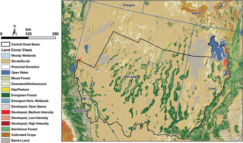
The landscape drains internally, and playa lakes are relatively common. Well-known lakes include Mono Lake and the Great Salt Lake. Numerous smaller cities and towns dot the landscape, but much of the area is devoid of human habitation. Portions of two large metropolitan statistical areas are located on the study area’s eastern and western edges: Salt Lake City and Reno-Sparks.

2.2. Data

2.2.1. eMODIS NDVI data and preparation

The eMODIS NDVI (https://earthexplorer.usgs.gov/) is a derivative of MODIS data acquired by the Terra and Aqua satellites that are operated by NASA. We use data from the Terra satellite. eMODIS is useful for trend analysis and near-real-time studies and is available at 250, 500, and 1000-m spatial resolutions. eMODIS NDVI is a 250-m spatial resolution product that is created using the MODIS red and near-infrared (NIR) surface reflectance data (Table 1) in a simple normalization (Equation (1)) (Jenkerson, Maiersperger, and Schmidt 2010). NDVI is a commonly used index in remote-sensing vegetation studies because it distinguishes vegetation from bare ground and snow cover and provides a measure of vegetation vigor and dynamics (Jensen 2005; Ke et al. 2015). The normalized difference of the red and infrared spectral channels helps eliminate a portion of the noise inherent to remotely sensed data. Therefore, when examining vegetation conditions, the NDVI provides a stable spatial and temporal record of vegetation greenness (Hwang et al. 2011). The process that produces eMODIS NDVI uses a maximum-value-composite algorithm that identifies the best pixel in each 7-day period by filtering through input surface reflectance of poor quality, negative values, low view angles, clouds, and snow cover (Jenkerson, Maiersperger, and Schmidt 2010). These data are available in weekly, 7-day composites. Additionally, to mitigate the effects of possible residual cloud cover, we temporally smoothed the weekly composites using a weighted, least-squares approach. The temporal smoothing of the weekly NDVI can reliably interpolate across temporary drops in NDVI associated with residual clouds after the weekly best-pixel NDVI compositing (Swets et al. 2000). Together, the compositing and smoothing processes mitigated most cloud-caused data inconsistencies (Brown et al. 2015).

(1)

Table 1. Band characteristics for Terra MODIS NDVI and Landsat 8 Operational Land Imager.

	Band number		Spectral range (nm)
Band name	MODIS NDVI	Landsat 8	MODIS NDVI	Landsat 8
Red	1	4	620–670	630–680
Near-infrared	2	5	841–876	845–885
Blue	–	2	–	450–515
Green	–	3	–	525–600
Shortwave infrared 1	–	6	–	1560–1660
Shortwave infrared 2	–	7	–	2100–2300

where NIR and red represent the spectral reflectance measurements, respectively, in the NIR and red regions of the electromagnetic spectrum.

2.2.2. Landsat 8 composite data and preparation

We used tiled, best-pixel Landsat composites (bands 2–7) built with the Multi-Index Integrated Change Analysis method and used by the LANDFIRE Remote Sensing of Landscape Change process. These best-pixel composites were constructed from algorithm-driven, 30-m Landsat 8 Level 1T composite scenes with cloud cover of less than 80% (Nelson and Steinwand 2015). An algorithm to convert Landsat 8 Level 1T data to surface reflectance was unavailable when this study occurred. Therefore, the Landsat 8 data were converted to top-of-atmosphere reflectance (Nelson and Steinwand 2015). Two best-pixel composites, each built from as many as six consecutive dates of Landsat 8 data, were available for this study. These composites reflect (1) an early summer date centered on day-of-year (DOY) 175 with pixels that ranged from DOY 100 to DOY 199 and (2) a late summer date centered on DOY 250 with pixels that ranged from DOY 200 to DOY 299 (Nelson and Steinwand 2015). These best-pixel Landsat 8 tiles were developed primarily to mitigate cloud and shadow issues that can contaminate individual Landsat scenes. These two composites of Landsat 8 data were averaged spatially using a 7 × 7 moving window. This process assigns each 30-m pixel a value using the average of the nearest 49 pixel values to produce a more accurate representation of the 250-m data. We then resampled the Landsat best-pixel composites to 250 m using nearest neighbor to match the spatial resolution of the eMODIS NDVI data.

2.2.3. Data selection and use

We downscaled temporally smoothed, composited images of 250-m eMODIS NDVI with best-pixel Landsat composite tiles to create 30-m satellite-based datasets that mitigated cloud and shadow contamination and captured seasonal vegetation dynamics. The downscaled eMODIS NDVI represented 4 weeks from the year 2013 and served as independent variables in independently developed sagebrush ecosystem models for 2014. These models were designed to predict sagebrush ecosystem land-cover types as fractional components that included herbaceous plants and shrubs (Xian et al. 2015; Homer et al. 2012). Landsat data in best-pixel format (Nelson and Steinwand 2015) were not available for 2014 at the time of processing for this study, so we downscaled 2013 eMODIS NDVI data using 2013 best-pixel Landsat data. We understood that 2 years of NDVI values could differ substantially because of annual disturbances, management, and weather effects on plant phenology and growth, and that these differences could affect how the 2014 sagebrush ecosystem model responded to these 2013 downscaled eMODIS NDVI variables.

Dates of eMODIS NDVI weekly composites selected for downscale complemented the Landsat data that were used in the sagebrush ecosystem models. These Landsat data (different from the best-pixel Landsat composites described above) used in the sagebrush ecosystem models blended multiple dates of Landsat images to mitigate cloud and shadow effects. The eMODIS NDVI composites targeted phenological periods in 2013 that were important for distinguishing rangeland vegetation types in the central Great Basin. These weeks of NDVI represented spring (mean of weeks 17 and 18) to capture annual grass greenness and early summer (week 27) to capture annual grass senescence. The weeks of downscaled NDVI also represented late summer (week 37) to differentiate between sagebrush (Artemisia) and other shrubs’ phenologies and fall (week 43) to differentiate sagebrush, which does not lose all leaves, from other shrubs that do lose all leaves (Figure 2 and Table 2). We used arrows in Figure 2 to indicate the weeks of NDVI selected above and describe in the caption why these dates were chosen. We used brackets to show the range of dates for the Landsat data that were blended for the sagebrush ecosystem models.

Table 2. Downscaled eMODIS NDVI ecological periods identified by week of year, the corresponding calendar period, and season for the year 2013.

Week	Calendar period	Season
17 and 18^a	21 April–4 May	Spring
27	30 June–6 July	Early summer
37	8–14 September	Late summer
43	20–26 October	Fall

Note: ^aWe use the eMODIS NDVI mean value of weeks 17 and 18.

Figure 2. Average 2013 eMODIS NDVI profiles of some rangeland vegetation classifications in the study area. We used this chart to identify 4 weeks of ecological interest for downscaling eMODIS NDVI based on the timing of vegetation phenology. We also considered the dates of blended Landsat data that are collected for the sagebrush ecosystem models. The arrows identify the weeks of interest for downscaling eMODIS NDVI and correspond to weeks 17 and 18, 27, 37, and 43. The arrow at weeks 17 and 18 shows when the study area’s average annual herbaceous greenness neared its peak, a profile it maintained for approximately 6 weeks. The arrow at week 27 points to a flattening of that profile and indicates the end of annual herbaceous plant senescence. The optimal time to distinguish between the all-sage and the non-sage shrub using remote sensing occurred at week 37 when the difference between these two vegetation types’ profile was greatest. Week 43 began the flattening of the all-sage profile, a time when sagebrush contained the fewest leaves and other shrubs had none. This flattening persisted until about week 48 when the profile dipped precipitously, likely the result of snow contaminating the satellite scenes. The brackets enclose the dates of blended Landsat images and correspond to weeks 20–23, weeks 26–30, and weeks 34–38.

2.3. Model and map development

Cubist® (RuleQuest 2008) regression-tree software was used to build rule-based models that incorporated the spatially averaged 250-m Landsat 8 composites as independent variables to predict the dependent variable as a continuous variable (Quinlan 2008) (Figure 3). All models included five committees (similar to a boosted tree), and each committee had a set number of rules. Table 3 shows the average number of committee rules per model. Models trained on a wide range of environmental and ecological conditions that use a large number of training points create robust models that achieve the best results (Gu et al. 2012). In the current study, we extracted data from more than 124,000 randomly stratified points each for four regression-tree models. The training data were stratified so that each training value contributed a minimum of 10–20 training points unless that many points did not exist at a value. If enough points at a specific value did not exist, then the model used all available points at that value for training.

Table 3. Variable usage frequency, structure, and accuracy metrics for the four models.

Model weeks									Variable
Driving variables	17 and 18		27		37		43		Average
DOY and Landsat 8 bands
D175 band 2 (Blue)	41	97	76	95	74	88	65	88	78
D175 band 4 (Red)	85	85	63	99	20	95	61	92	75
D250 band 4 (Red)	16	98	40	92	67	99	72	98	73
D175 band 5 (NIR^a)	77	99	37	99	18	90	49	88	70
D175 band 6 (SWIR^b 1)	46	88	48	68	27	84	58	82	63
D250 band 5 (NIR)	12	75	13	96	39	100	59	98	62
D175 band 3 (Green)	52	98	10	99	5	97	5	90	57
D250 band 3 (Green)	5	96	–	96	4	90	1	91	55
D175 band 7 (SWIR 2)	29	87	2	85	–	71	11	94	54
D250 band 6 (SWIR 1)	6	83	–	71	2	87	7	93	50
D250 band 2 (Blue)	10	87	4	95	3	95	4	78	47
D250 band 7 (SWIR 2)	18	73	2	71	11	83	22	99	47
D175 average usage	55	92	39	91	24	88	42	89	66
D250 average usage	11	85	10	87	21	92	28	93	56
Model weeks	17–18		27		37		43
Model structure	5 committee		5 committee		5 committee		5 committee
Average rules per committee	89		52		30		127
Training points (n)	124,079		128,649		127,170		128,669
Test points (n)	9901		10,250		10,149		10,250
Training R^2	0.85		0.81		0.74		0.76
Average absolute error	2.1		1.7		2.2		2.5
Relative absolute error	0.34		0.32		0.42		0.41
Training cross-validation R^2	0.85		0.81		0.74		0.74
Test R^2	0.85		0.83		0.74		0.77
Average absolute error	2.2		1.6		2.1		2.4
Relative absolute error	0.35		0.33		0.42		0.41

Notes: ^aNear-infrared.

^bShortwave infrared.

The table shows the frequency (%) that each driving variable is used in each model to stratify rules (boldface numerals) and to develop algorithms (light-faced numerals). Dashes indicate variable not used. The rightmost column shows average model usage for each band. Average error equals the mean difference of the actual and predicted values at all training or test points. The relative error magnitude is the ratio of the average error magnitude to the error magnitude that results from always predicting the mean value. A useful model requires a relative error of less than one. Cross-validation represents 10 holdout cases run independently and averaged.

Figure 3. A schematic that identifies the data and illustrates the process to downscale 250-m eMODIS NDVI using Landsat 8 Operational Land Imager (OLI) data.

The spring model targeted annual grasses. Therefore, training points for the spring model were limited to elevations less than or equal to 2133 m. We chose this threshold based on previous cheatgrass percent cover work where we found that, as a dominant annual grass, cheatgrass covered an average of less than 2% of the land area at elevations between 1750 and 2000 m in the northern Great Basin (Boyte, Wylie, and Major 2016). For the other three downscaled models, points above 2133 m were allowed but limited to approximately 2.5% of the training and test datasets to eliminate potential model bias. Otherwise, the four models were trained on pixels where the 2011 National Land Cover Database (The National Land Cover Database 2011) classified the pixel as greater than or equal to 70% shrub/scrub, herbaceous, or bare ground and where tree canopy was less than 30%. Pixels in these classifications represent likely rangelands. In addition, if both DOY 175 and DOY 250 Landsat 8 images had no data or a zero value (clouds or water) in the same pixel, we excluded that pixel as a training point.

The rule-based, regression-tree models built parameters and algorithms at 250 m based on the relationships between the variables by partitioning the data into information subspaces (rules), rules that were each fit with a linear-regression equation (Wylie et al. 2007). We show, as an example, the model output of one stratification and its associated algorithm. In our training dataset, 2000 training cases meet the following criteria where all “bands” are Landsat 8 data used as independent variables:

if  Band 01 > 758 and  Band 01 ≤ 1303 and  Band 09 > 1434then  eMODIS NDVI prediction = 123.2–0.0359 (band 09)    + 0.0246 (band 10) − 0.0176 (band 01)  +0.0137 (band 02) + 0.0118 (band 07) + 0.0045 (band 06)    − 0.00341 (band 05)  −0.0034 (band 12) − 0.0021 (band 08) − 0.0003 (band 03)    − 0.0002 (band 11)

The 2000 training cases prediction: mean = 124.4, range 107–189, average estimated error = 3.2.

These rules and their associated linear equations were input along with the original 30-m Landsat 8 rasters into mapping software. The mapping software applied these rule-based parameters and algorithms from the 250-m models to the best-pixel composited, 30-m Landsat 8 rasters and generated spatially explicit, 30-m eMODIS NDVI predictions that estimated NDVI for each of the four weekly periods. These datasets are available at Boyte et al. (2017).

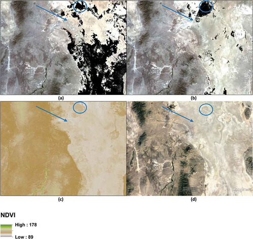
Figure 4 illustrates an advantage of the regression-tree approach – the ability of the regression-tree model and mapping process to ameliorate effects from less-than-optimal input data. The Landsat 8 composite for DOY 175  (Figure 4(a)) shows numerous pixels flagged as cloud or cloud shadow (black areas having no data). The eMODIS NDVI prediction did not carry over these values; instead, its prediction was based on the DOY 250 data. This resulted in a prediction much more reflective of the Google Earth image (Figure 4(d)). The arrow in the DOY 250 Landsat composite (Figure 4(b)) points to a distinct line where disparate dates of imagery were merged to create the composite. No line was visible in the same area in the DOY 175 Landsat (Figure 4(a)) composite. The eMODIS NDVI prediction (Figure 4(c)) shows no evidence of this line, which was contrary to what occurred when the STARFM approach was used in similar circumstances (Walker et al. 2012). In addition, the blue circle in Figure 4 encompasses an area where both DOY 175 and DOY 250 Landsat composites experienced no data values (no training points were cast in this area). The corresponding area in the eMODIS NDVI prediction showed reasonable NDVI values for this area in a pattern that resembled the overlapping no-data values from the two composites. This finding strongly suggests that, in some instances, when the regression-tree model was optimally parameterized (Gu et al. 2016), the modeling and mapping processes eliminated the effects of spatial artifacts and mitigated no-data values that occurred in input data.

Figure 4. A subset of 1 week of the eMODIS NDVI prediction compared to the Landsat 8 best-pixel composite images used as model drivers, with Google Earth as a reference. The arrow and circle highlight problem areas with input data, a line caused by compositing Landsat data in one image and no data values in both images. The eMODIS NDVI prediction mitigates these issues, showing no evidence of a composite line and predicting reasonable NDVI values in place of no data values. The eMODIS NDVI was scaled from the typical −1–1 scale. The new scale is 0–200 (100x + 100) to remove the data requirement to store negative values. The center coordinates for the images equal approximately 113°57′7.1″W 40°17′2.2″N. (a) Landsat 8 best-pixel composite DOY 175 (Bands 2–4), (b) Landsat 8 best-pixel composite DOY 250 (Bands 2–4), (c) week 17-18 eMODIS NOVI predicted (30 m), (d) Google Earth image – May and October 2013.

2.4. Model and map validation and assessment

Model outputs included accuracy assessments that compared training and test data values with corresponding predicted values. Accuracy assessment metrics included correlation coefficient (r), average absolute error, and relative absolute error for both training and test datasets. The relative error magnitude was the ratio of the average error magnitude compared with the error magnitude that resulted from always predicting an average value. Useful models experienced relative errors less than one (Quinlan 2008). The test data were independent from the training data that were used to develop rules, algorithms, or parameters that predicted the dependent variable. Consequently, the test dataset provided a measurement of the data “unseen” by the model, an independent test of model accuracy. We also performed separate cross-validations of each model with 10-folds (equal-sized subsets) where training datasets were divided randomly. For each model, nine of the folds predicted the target values while onefold served as a test. This process was repeated 10 times such that every observation was used as a test once. The average of the mean absolute error across all 10-folds provided the random cross-validation accuracy assessment metric.

The downscaled 30-m eMODIS NDVI spatially explicit datasets were added to the sagebrush ecosystem models to improve predictions. We evaluated the effects that these downscaled datasets had on several of the sagebrush ecosystem models, measuring the difference in sagebrush ecosystem-model metrics when these downscaled datasets were and were not included as independent variables. The components of the sagebrush ecosystem models included annual herbaceous, bare ground, herbaceous, litter, sagebrush, and non-sage shrub (Table 4). Two assessments were undertaken. First, both versions of each of the six sagebrush ecosystem model outputs were validated using 135 points of independently gathered field data. Independent validation points were located within randomly selected 7-km radius sites. In each site, we randomly placed 9–10 points in non-forested areas within 750 m of the nearest road. Second, each model was cross validated at 40,000 data points. Metrics used to evaluate the comparison of these models included the range of each component’s values, the coefficient of determination (R²), and the root mean squared error (RMSE).

Table 4. Changes in independent (n = 135) and cross-validation (n = 40,000) statistical metrics associated with the addition of various downscaled eMODIS NDVI images as independent variables in component regression-tree models.

	Weeks 17, 18 and 27			Weeks 17, 18 and 43			All weeks^a
	Metric			Metric			Metric
Model component	ΔRange	ΔR^2	ΔRMSE	ΔRange	ΔR^2	ΔRMSE	ΔRange	ΔR^2	ΔRMSE
Ind. validation
Annual herb.	1	0.02	−0.10	–	–	–	–	–	–
Bare ground	3	−0.01	0.00	4	−0.03	0.00	0	−0.04	0.01
Herbaceous	−5	−0.03	0.14	2	−0.04	−0.01	6	−0.16	0.00
Litter	0	0.00	0.04	–	–	–	–	–	–
Sagebrush	−1	−0.04	0.27	–	–	–	–	–	–
Non-sage shrub	−1	−0.17	0.00	0	0.01	0.00	−5	−0.14	0.07
Cross-valid.
Annual herb.	−1	0.00	−0.01	–	–	–	–	–	–
Bare ground	1	0.00	−0.07	0	0.01	−0.10	−1	−0.17	3.07
Herbaceous	0	0.00	−0.02	0	0.00	−0.01
Litter	1	0.01	−0.07	–	–	–	–	–	–
Sagebrush	2	0.00	−0.01	–	–	–	–	–	–
Non-sage shrub	−3	0.00	−0.04	0	0.01	−0.17	−19	−0.23	2.05

Notes: ^aAll four downscaled dates: weeks 17 and 18, week 27, week 37, and week 43.

Changes are assessed relative to a version with no downscaled dates, with all other variables held constant. Weeks 17 and 18 and 43 and all tests were conducted only for bare, herbaceous, and shrub cover.

Additionally, we visually compared a few small sections of the eMODIS NDVI images at 250 and 30 m to highlight spatial differences in landscape features like center-pivot irrigation, roads, elevational changes, and fire effects on NDVI. We also visually evaluated NDVI, comparing seasonal changes in vegetation greenness. Finally, we statistically compared the original 250-m eMODIS NDVI to the predicted 30-m eMODIS NDVI after it was spatially averaged and resampled to 250 m. To do this statistical comparison, we accounted for possible image misregistration of remotely sensed data (daily MODIS images and Landsat scenes) in the sample population. Image shifts can cause unexpected results and have been especially acute when working with time series data. We accounted for image misregistration by developing a spatial coefficient of variation (CV) that we used to filter out sample pixels with high CV values (slight geographic misregistration in more uniform areas would cause negligible effects). Sample population pixels were eliminated if their CV values were at least three times greater than the mean CV value in the 250-m eMODIS NDVI prediction. The spatial averaging of the predictions generalized their 30-m outputs, but this method provided a direct evaluation of mapping accuracy.

3. Results

3.1. Variable usage, model structure, and accuracy assessment

The regression-tree models generated metrics that measured how frequently each variable was used to stratify model rules and to develop model algorithms. This model transparency allowed the identification of variables most influential to model development for the downscaled predictions (Table 3). Overall, algorithm development (light-faced numerals in Table 3) used variables far more frequently than did rules stratification (bold-faced numerals in Table 3), although the DOY 175 red band was used equally for both activities (85%) during weeks 17 and 18. The NIR band from DOY 175 was used, on average, more frequently for weeks 17 and 18 (88%) than any other variable. The average of all weeks for the DOY 175 blue band (78%) was higher than the average of all weeks for any other variable. The DOY 175 blue band was used slightly more often than the red bands from Day 175 (75%) and Day 250 (73%). The blue and the shortwave infrared 2 bands from DOY 250 (47%) tied for least frequently used variables in model development. On average, variables from DOY 175 (66%) were used more often than variables from DOY 250 (56%). The two strongest models built were for weeks 17 and 18 and week 27. Weeks 17 and 18 experienced the highest test R² (0.85), while week 27 experienced the lowest test average absolute error (1.7) and the lowest test relative absolute error (0.32). The week 37 and week 43 models were relatively strong with test absolute average errors equal to 0.42 and 0.41, respectively. Each model developed was useful with strong to very strong R² values and low average absolute and relative absolute errors. The R² test dataset values equaled the R² training dataset values in weeks 17 and 18 and week 37 and slightly exceeded the training R² values for week 27 and week 43. These results suggest well-fitted models.

Accuracy metrics for the sagebrush ecosystem models that included and excluded downscaled 2013 eMODIS NDVI images are displayed in Table 3. Mixed results occurred when using these data as independent variables for the 2014 sagebrush ecosystem models, although only a few results showed dramatic improvement or degradation. When downscaled NDVI data from weeks 17 and 18 and week 27 were used, the model that predicted annual herbaceous cover improved in all metrics. The range increased by 1, the R² increased by 0.02, and the RMSE declined by 0.10. However, the models that predicted sagebrush and herbaceous cover, which included both annual and perennial herbaceous, each experienced degradation in all metrics when using weeks 17 and 18 and week 27 downscaled eMODIS NDVI. The range of herbaceous cover expanded when week 43 was substituted for week 27 and when all four weekly downscaled images were included. The cross-validation statistics showed improved RMSEs for all six components when NDVI from weeks 17 and 18 and week 27 were added to the models but had a negligible effect on their R² values. The effect on the model was negligible when the non-sage shrub model included the downscaled image from weeks 17 and 18 and week 43. Any of the models that used all four downscaled dates experienced reduced R² and RMSE values.

Comparing the original eMODIS NDVI data to corresponding predicted 250-m eMODIS NDVI mapping outputs showed strong relationships. Across 932 sample points on the weeks 17 and 18 scatterplot (Figure 5(a)), the data mostly were tightly clustered around the regression and the 1:1 lines with few exceptions, and the R² was 0.83. Table 5 shows the RMSE was 3.37, and the nRMSE was 0.06. The nRMSE is the normalized RMSE, a dimensionless statistic that removes the effects of a dataset’s range from the metric (Homer et al. 2012). The scatterplots for week 27 (Figure 5(b)), week 37 (Figure 5(c)), and week 43 (Figure 5(d)) included sample points (open circles) above an elevation threshold of 2133 m. The week 27 correlation coefficient (0.91) matched that of weeks 17 and 18, but the week 27 RMSE and nRMSE were lower (3.05, 0.03) (Table 5), showing better agreement between the original and the predicted eMODIS NDVI. The higher elevation points in week 27 were mostly restricted to lower NDVI values, with a maximum value of 147 and a range of 37 (the eMODIS NDVI is scaled 100x + 100 to remove negative values). This restriction of higher elevation points to lower NDVI values was less pronounced in week 37 and week 43 scatterplots where maximum values were higher and the range of values was broader. The outliers in weeks 17 and 18 were mostly overpredictions, whereas most outliers in week 37 and week 43 were underpredictions. Week 27 experienced outliers, both as underpredictions and overpredictions. All regression lines fell extremely close to their corresponding 1:1 lines.

Table 5. Statistics describing the relationship between the original 250-m eMODIS NDVI datasets and the predicted 30-m eMODIS NDVI datasets that are spatially averaged and resampled to 250 m.

Statistic	Week 17 and 18	Week 27	Week 37	Week 43
r	0.91	0.91	0.91	0.89
Linear equation	y = 0.942x + 6.9298	y = 0.9696x + 4.1027	y = 1.004x − 0.2529	y = 0.9639x + 4.4826
RMSE	3.37	3.04	2.72	3.61
nRMSE	0.06	0.03	0.04	0.08
Sample points ≤2133 m	932	924	938	920
Sample points >2133 m	Not applicable	57	72	97

Note: The nRMSE is the normalized root mean squared error, a dimensionless statistics that removes the effects of a dataset’s range of values.

Figure 5. Scatterplots comparing original 250-m eMODIS NDVI datasets with predicted 30-m eMODIS NDVI datasets that are spatially averaged and resampled to 250 m. We trained the model for the weeks 17 and 18 (a) at or below an elevation of 2133 m (~7000 ft); therefore, this weeks’ analysis includes no sample points cast above this elevation. Two models each for weeks 27 (b), 37 (c), and 43 (d) are trained, one at or below elevations equal to 2133 m and the other above 2133 m. The solid black lines are 1:1 lines and the dashed lines are regression lines. Solid circles represent sample points at or below 2133 m and open circles represent sample points above 2133 m. See Table 5 for statistics that describe the relationships between datasets for each week.

3.2. Visual comparison of 250 and 30-m eMODIS NDVI

Figure 6(a–h) shows the same geographic space, and these images allowed visual comparison of a small section of the four original 250-m eMODIS NDVI to the four corresponding modeled 30-m eMODIS NDVI predictions. These visual comparisons included an evaluation of vegetation greenness for each week that we modeled. Additionally, the weeks 17 and 18 images provided an example of how the selection of model training points influenced mapping accuracy. As stated earlier, we intentionally did not train the weeks 17 and 18 model at elevations above 2133 m; therefore, we did not calibrate the model to conditions above this threshold. In the upper left corner of the original 250-m image (Figure 6(b)), where elevations were higher than 2400 m, very low NDVI values were present, indicating the presence of no vegetation greenness (gray shaded area). In fact, much of the ground cover was likely snow. In the same area of the corresponding 30-m prediction (Figure 6(a)), most of the NDVI values were much higher, indicating substantial vegetation greenness with some bare ground, but no snow. The error in the 30-m prediction map occurred because of the lack of model calibration at elevations above 2133 m. This same error was not repeated in the predictions of the three other weeks because their models included training points above 2133-m elevation.

Figure 6. An illustration of spatial detail gained by modeling and mapping eMODIS NDVI through time with Landsat 8 bands as drivers. All images have the same extents, adjusted for spatial resolution. The center coordinates for the images equal approximately 115°23′31.5″W 40°24′40.8″N and include part of the Ruby Mountains, Nevada. The eMODIS NDVI is scaled (100x + 100) to remove negative values; therefore, a value of 100 on one of the images above would equal a normally scaled NDVI value of 0. We set our model to allow 5% extrapolation; therefore, values greater than 200 can occur. (a) Week 17–18 eMODIS NDVI predicted (30 m), (b) week 17–18 original eMODIS NDVI (250 m), (c) week 27 eMODIS NDVI predicted (30 m), (d) week 27 original eMODIS NDVI (250 m), (e) week 37 eMODIS NDVI predicted (30 m), (f) week 37 original eMODIS NDVI (250 m), (g) week 43 eMODIS NDVI predicted (30 m), (h) week 37 original eMODIS NDVI (250 m).

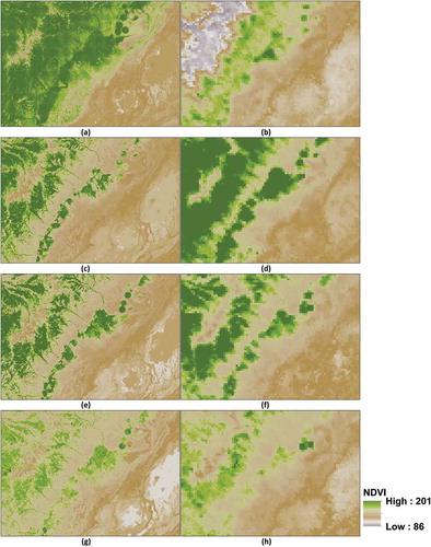
The general spatial trends matched between the images in Figure 6, but the level of spatial detail was remarkable in the 30-m predictions when compared to the 250-m eMODIS NDVI. Center-pivot agriculture artifacts were clearly discernible as round green features in all 30-m images, whereas in the 250-m images, these artifacts appeared as squares that do not resemble center-pivot irrigation. In Figure 6(a), a road was clearly visible through the center of the image (the road was much more difficult to see in the other 30-m images because the NDVI values in the immediate area do not provide a contrast for the road). This road was not distinguishable in any 250-m image. Channels that divert water runoff from higher ground were evident in the 30-m images. These channels provide more mesic environments that promote vegetation growth and greenness during the growing season, hence the higher NDVI values. These channels were considerably more difficult to recognize and much less detailed in the 250-m images because of their substantially lower spatial resolutions. Seasonal differences also were detected in the greenness of the images (note that Figure 6(a) exaggerated greenness at higher elevations). Early and late growing season periods (Figure 6(b), (g–h), respectively) showed less greenness than the middle of growing season period (Figure 6(c–f)) because of the timing of these images. Missing from the images in Figure 6 were visible residuals from cloud, shadow, and atmospheric contamination. The widths of the red and NIR bands along with the compositing and temporal smoothing of the eMODIS NDVI mitigated these problems, which can affect any remotely sensed product. Artifacts of these issues were not evident in these images.

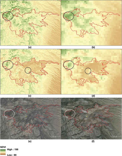
In Figure 7, the red polygon, downloaded from the Monitoring Trends in Burn Severity website (http://www.mtbs.gov/data/individualfiredata.html), shows the boundary of the Black Fire that occurred in eastern Nevada on 1 July 2013. Figure 7 compares prefire images (Figure 7(a,b)) with postfire images (Figure 7(c,d)) at different resolutions. This comparison shows changes in NDVI that typically occurred after fire in vegetated areas. The Google Earth images (Figure 7(e,f)) provided a point of reference for pre- and postfire dynamics. Low NDVI values, representing low or no vegetation greenness, dominated much of the postfire images, as expected, but the 30-m predicted image offered more spatial detail about fire severity and better identified potentially unburned areas. The circled areas, especially in the center of images Figure 7(c,d), are examples of where the 30-m predictions provided substantially more detail than the 250-m images, illustrating the fire’s effects on vegetation.

Figure 7. An illustration of fire effects on vegetation greenness as calculated by NDVI and spatial differences of the predicted (30 m) and original (250 m) eMODIS NDVI. The red polygon, downloaded from the Monitoring Trends in Burn Severity website (http://www.mtbs.gov/data/individualfiredata.html), shows the fire boundary for the Black Fire in eastern Nevada. The fire date was 1 July 2013, at the start of week 27’s compositing period (see Table 1). Dark areas on a prefire Google Earth image from September 2010 represent trees. Many previous dark areas inside the polygon are void of trees and other vegetation and appear lighter in the post fire, August 2014, Google Earth image. The circles show an example of vegetation change at different spatial scales. All images have the same extents, adjusted for spatial resolution. Center coordinates for the images equal approximately 114°11′52.33″W 38° 50′12.87″N. (a) Week 27 eMODIS NDVI predicted (30 m), (b) week 27 eMODIS NDVI original (250 m), (c) week 37 eMODIS NDVI predicted (30 m), (d) week 37 eMODIS NDVI original (250 m), (e) Google Earth image – September 2010, (f) Google Earth image – August 2014.

4. Discussion

The regression-tree process developed 30-m synthetic eMODIS NDVI using Landsat and atmospherically corrected eMODIS NDVI data (Jenkerson, Maiersperger, and Schmidt 2010). This process is unlike the STARFM, the enhanced STARFM, and STAARCH, which all generate synthetic Landsat images using Landsat and MODIS data (Gao et al. 2006; Tewes et al. 2015; Gao et al. 2015). The regression-tree algorithms included many terminal nodes (stratified prediction end points) where specific independent variable combinations were applied to optimize predictions (De’ath and Fabricius 2000). The regression-tree software looked for a set of independent variables that for each terminal node helped predict eMODIS NDVI on the target date most accurately. For example, the Landsat 8 blue band is sensitive to atmospheric effects, and the Landsat scenes that make up the DOY 175 best-pixel composite likely experienced frequent cloud cover. This would have caused the low usage of the DOY 175 blue band in stratifying predictions for weeks 17 and 18. During the later weeks that we downscaled, cloud cover and other atmospheric factors may not have occurred as frequently and, consequently, the DOY 175 blue band was used by the regression-tree software much more frequently to stratify rules and slightly less frequently to build prediction algorithms. Ollinger (2011) notes that the infrared band is the strongest component in the NDVI formula, accounting for about 60% of the NDVI signature and the red band accounting for the rest. Therefore, we expect that the NIR and red bands would contribute strongly to the models’ predictions of eMODIS NDVI, which they do. Overall, these bands are four of the six most frequently used Landsat bands in models for DOYs 175 and 250.

To develop robust models, the models were trained on large datasets that represented a wide range of environmental and ecological conditions across the study area. Model robustness was manifested by the test data experiencing almost identical accuracy values to the training data values (Table 3). Since the test data were independent of model development, the accuracy of the test data suggested that the model would perform well on “unseen” data. Week 27 and week 37 predictions experienced the lowest RMSEs and nRMSEs of the four downscaled weeks when compared to original eMODIS NDVI data (Figure 5 and Table 5). Their sample point correlation coefficients (r = 0.91) were similar to their models’ accuracies and equaled that of weeks 17 and 18 and the downscaled GSN model that Gu and Wylie (2015a) produced for central Nebraska. This downscaled GSN model found the best accuracy of growing season MODIS NDVI when the Landsat scenes that downscaled the MODIS NDVI came from the early, middle, and late growing seasons. In the current study, week 27 and week 37 occurred immediately after the dates of the DOY 175 and DOY 250 Landsat composites, which suggests that the nearer the original eMODIS NDVI dates are to the dates of the Landsat 8 composites, the more effective the downscaling process.

The phenological trends discussed in the visual comparison part of Section 3 reflected an understanding of the general timing of rangeland vegetation-type greenness in this geographic area. Vegetation growth peaked during early to late summer, and these peaks were visible in the week 27 and week 37 images (Figure 6(c–f)) and were in relative contrast with the weeks 17 and 18 (Figure 6(b)) and week 43 (Figure 6(g,h)) images. Figure 7 demonstrated expected vegetation responses to fire as illustrated by the lower NDVI values presented in much of the postfire image when contrasted with the prefire image. In the context of this study, the spatial detail of the downscaled eMODIS NDVI was most important because areas of remaining vegetation could be distinguished in the 30-m prediction that were not distinguishable in the original 250-m eMODIS NDVI image. This increased spatial detail provides more information to the user.

Validation of the sagebrush ecosystem mapping models indicated improvement in the annual herbaceous model (Table 4) when weeks 17 and 18 and week 27 downscaled eMODIS NDVI images were included as variables, and this corresponds with expectations. Annual herbaceous growth would likely have been active in the central Great Basin for most of the time during and between these two weeks, and the model’s usage of these downscaled images was reflected in a modest change in accuracy metrics. In contrast, the all-sage ecosystem model and the non-sage shrub ecosystem model experienced degradation when downscaled images from weeks 17 and 18 and week 27 were included. Active shrub growth during these periods likely was minimal, especially during weeks 17 and 18, and at higher elevations even after weeks 17 and 18. When the week 43 downscaled image was added to the non-sage shrub model and used along with the weeks 17 and 18 image, the effect on the model was negligible. Inclusion of weeks 17 and 18 and week 27 images improved RMSE values for all sagebrush ecosystem models’ cross-validation statistics but had a negligible effect on their R² values. Any of the sagebrush ecosystem models that included all four downscaled dates experienced reduced accuracy metrics, especially when considering cross-validation statistics. What this study could not answer definitively was whether the downscaled eMODIS NDVI could improve the sagebrush ecosystem models appreciably. One substantial caveat must be acknowledged when considering this analysis; Landsat best-pixel composites from 2014 were unavailable for model development and analysis, so 2013 Landsat best-pixel composites were used to downscale 2013 eMODIS NDVI datasets. These downscaled 2013 eMODIS NDVI were ingested into the 2014 sagebrush ecosystem models. Using downscaled data from the same year as the sagebrush ecosystem models may have improved mapping accuracies. The same weather patterns, disturbances, and management decisions that affected the sagebrush ecosystem models would have affected the downscaled eMODIS NDVI inputs.

5. Conclusion

This study demonstrated that regression-tree modeling software can be used to downscale 250-m eMODIS NDVI data using 30-m Landsat 8 OLI data relatively easily and effectively. The integration of data into regression-tree modeling software from these two satellites exploited different characteristics of each and helped to mitigate each satellite’s limitations. This facilitated a better understanding of seasonal rangeland dynamics in the central Great Basin by downscaling images with atmospheric corrections, greater spatial resolution that improved image detail, and enhanced temporal resolution that allowed the analysis of short-lived plants with rapidly changing phenologies. The result of this modeling and mapping process also highlighted fire effects on rangelands, providing detail that was unattainable using data from only one sensor. For future studies, we identified one potential residual benefit to the modeling process demonstrated in this study; we think it is possible to create 30-m maps of atmospherically corrected synthetic eMODIS NDVI, driven by Landsat inputs, for any 7-day period from 1982 (the launch of Landsat 4) to the present. This effort would require testing a multiple-year, historical regression-tree model built to emulate historical environmental conditions. The model would create parameters and algorithms that could be applied to the mapping application along with Landsat data that predate the launch of MODIS. This process would produce 30-m eMODIS NDVI predictions that could match with previous dates of field data and/or coincide with important phenology dates. This effort would allow telling a more complete story of rangeland seasonal dynamics in the central Great Basin.

Acknowledgments

Thanks are due to many people for the development of this manuscript. The authors thank Jennifer Rover, Thomas Adamson, and the anonymous journal reviewers for constructive recommendations that made this manuscript better; the US Geological Survey sagebrush ecosystem team for sharing data and for testing the downscaled models’ mapping outputs by incorporating them into the sagebrush ecosystem model; and Kurtis Nelson for providing the Landsat 8 composited tiles.

Disclosure statement

The authors declare no conflicting interests. Any use of trade, firm, or product names is for descriptive purposes only and does not imply endorsement by the US government.

Additional information

Funding

The US Bureau of Land Management and the U.S. Geological Survey Land Change Science program funded this work.

References

- Atkinson, P. M. 2013. “Downscaling in Remote Sensing.” International Journal of Applied Earth Observation and Geoinformation 22 (1): 106–114. doi:10.1016/j.jag.2012.04.012.
- Balch, J. K., B. A. Bradley, C. M. D’Antonio, and J. Gómez-Dans. 2013. “Introduced Annual Grass Increases Regional Fire Activity across the Arid Western USA (1980–2009).” Global Change Biology 19 (1): 173–183. doi:10.1111/gcb.12046.
- Boyte, S. P., B. K. Wylie, and D. J. Major. 2016. “Cheatgrass Percent Cover Change: Comparing Recent Estimates to Climate Change - Driven Predictions in the Northern Great Basin.” Rangeland Ecology and Management 69 (4): 265–279. doi:10.1016/j.rama.2016.03.002.
- Boyte, S. P., B. K. Wylie, D. J. Major, and J. F. Brown. 2015. “The Integration of Geophysical and Enhanced Moderate Resolution Imaging Spectroradiometer Normalized Difference Vegetation Index Data into a Rule-Based, Piecewise Regression-Tree Model to Estimate Cheatgrass Beginning of Spring Growth.” International Journal of Digital Earth 8 (2): 118–132. doi:10.1080/17538947.2013.860196.
- Boyte, S. P., B. K. Wylie, M. B. Rigge, and D. Dahal. 2017. “Estimating Downscaled eMODIS NDVI Using Landsat 8 in the Central Great Basin Shrub Steppe.” U.S. Geological Survey Data Release. doi:10.5066/F7R20ZVX.
- Bradley, B. A., and J. F. Mustard. 2005. “Identifying Land Cover Variability Distinct from Land Cover Change: Cheatgrass in the Great Basin.” Remote Sensing of Environment 94 (2): 204–213. doi:10.1016/j.rse.2004.08.016.
- Bradley, B. A., and J. F. Mustard. 2006. “Characterizing the Landscape Dynamics of an Invasive Plant and Risk of Invasion Using Remote Sensing.” Ecological Applications 16 (3): 1132–1147. doi:10.1890/1051-0761(2006)016[1132:CTLDOA]2.0.CO;2.
- Brown, J. F., D. M. Howard, B. K. Wylie, A. Frieze, L. Ji, and C. Gacke. 2015. “Application-Ready Expedited MODIS Data for Operational Land Surface Monitoring of Vegetation Condition.” Remote Sensing 7 (12): 16226–16240. doi:10.3390/rs71215825.
- Chang, N. B., K. Bai, and C. F. Chen. 2017. “Integrating Multisensor Satellite Data Merging and Image Reconstruction in Support of Machine Learning for Better Water Quality Management.” Journal of Environmental Management 201: 227–240. doi:10.1016/j.jenvman.2017.06.045.
- Commission for Environmental Cooperation. 2009. North American Terrestrial Ecoregions Level III. Montreal: Commission for Environmental Cooperation.
- De’ath, G., and K. E. Fabricius. 2000. “Classification and Regression Trees: A Powerful yet Simple Technique for Ecological Data Analysis.” Ecology 81 (11): 3178–3192. doi:10.1890/0012-9658(2000)081[3178:Cartap]2.0.Co;2.
- French, N. H. F., L. L. Bourgeau-Chavez, M. J. Falkowski, S. J. Goetz, L. K. Jenkins, P. Camill III, C. S. Roesler, and D. G. Brown. 2013. “Remote Sensing for Mapping and Modeling of Land-Based Carbon Flux and Storage.” In Land Use and the Carbon Cycle, edited by D. G. Brown, D. T. Robinson, N. H. F. French, and B. C. Reed, 95–143. Cambridge: Cambridge University Press.
- Gao, F., T. Hilker, X. L. Zhu, M. C. Anderson, J. G. Masek, P. J. Wang, and Y. Yang. 2015. “Fusing Landsat and MODIS Data for Vegetation Monitoring.” IEEE Geoscience and Remote Sensing Magazine 3 (3): 47–60. doi:10.1109/Mgrs.2015.2434351.
- Gao, F., J. Masek, M. Schwaller, and F. Hall. 2006. “On the Blending of the Landsat and MODIS Surface Reflectance: Predicting Daily Landsat Surface Reflectance.” IEEE Transactions on Geoscience and Remote Sensing 44 (8): 2207–2218. doi:10.1109/Tgrs.2006.872081.
- Gu, Y., D. M. Howard, B. K. Wylie, and L. Zhang. 2012. “Mapping Carbon Flux Uncertainty and Selecting Optimal Locations for Future Flux Towers in the Great Plains.” Landscape Ecology 27 (3): 319–326. doi:10.1007/s10980-011-9699-7.
- Gu, Y., and B. K. Wylie. 2015a. “Developing a 30-M Grassland Productivity Estimation Map for Central Nebraska Using 250-M MODIS and 30-M Landsat-8 Observations.” Remote Sensing of Environment 171: 291–298. doi:10.1016/j.rse.2015.10.018.
- Gu, Y., and B. K. Wylie. 2015b. “Downscaling 250-M MODIS Growing Season NDVI Based on Multiple-Date Landsat Images and Data Mining Approaches.” Remote Sensing 7. doi:10.3390/rs70403489.
- Gu, Y., B. K. Wylie, S. P. Boyte, J. Picotte, D. M. Howard, K. Smith, and K. J. Nelson. 2016. “An Optimal Sample Data Usage Strategy to Minimize Overfitting and Underfitting Effects in Regression Tree Models Based on Remotely-Sensed Data.” Remote Sensing 8: 943. doi:10.3390/rs8110943.
- Homer, C. G., C. L. Aldridge, D. K. Meyer, and S. J. Schell. 2012. “Multi-Scale Remote Sensing Sagebrush Characterization with Regression Trees over Wyoming, USA: Laying a Foundation for Monitoring.” International Journal of Applied Earth Observation and Geoinformation 14 (1): 233–244. doi:10.1016/j.jag.2011.09.012.
- Hwang, T., C. H. Song, P. V. Bolstad, and L. E. Band. 2011. “Downscaling Real-Time Vegetation Dynamics by Fusing Multi-Temporal MODIS and Landsat NDVI in Topographically Complex Terrain.” Remote Sensing of Environment 115 (10): 2499–2512. doi:10.1016/j.rse.2011.05.010.
- Jenkerson, C. B., T. K. Maiersperger, and G. L. Schmidt. 2010. “eMODIS—A User-Friendly Data Source.” In U.S. Geological Survey Open-File Report 2010-1055. U.S. Department of Interior: Reston, VA.
- Jensen, J. R. 2005. “Introductory Digital Image Processing: A Remote Sensing Perspective.” Prentice-Hall Series in Geographic Information Sciences. 3rd ed. Upper Saddle River, NJ: Pearson Prentice Hall.
- Ke, Y., J. Im, J. Lee, H. Gong, and Y. Ryu. 2015. “Characteristics of Landsat 8 OLI-derived NDVI by Comparison with Multiple Satellite Sensors and In-Situ Observations.” Remote Sensing of Environment 164: 298–313. doi:10.1016/j.rse.2015.04.004.
- Kennedy, R. E., S. Andréfouët, W. B. Cohen, C. Gómez, P. Griffiths, M. Hais, S. P. Healey, et al. 2014. “Bringing an Ecological View of Change to Landsat-Based Remote Sensing.” Frontiers in Ecology and the Environment 12 (6): 339–346. doi:10.1890/130066.
- Kennedy, R. E., P. A. Townsend, J. E. Gross, W. B. Cohen, P. Bolstad, Y. Q. Wang, and P. Adams. 2009. “Remote Sensing Change Detection Tools for Natural Resource Managers: Understanding Concepts and Tradeoffs in the Design of Landscape Monitoring Projects.” Remote Sensing of Environment 113 (7): 1382–1396. doi:10.1016/j.rse.2008.07.018.
- Kokaly, R. F. 2011. “DESI—Detection of Early-Season Invasives (Software-Installation Manual and User’s Guide Version 1.0).” In U.S. Geological Survey Open-File Report 2010-1302. U.S. Department of Interior: Reston, VA: U.S. Geological Survey Open-File Report 2010-1302.
- Lloyd, C. D. 2014. Exploring Spatial Scale in Geography, Exploring Spatial Scale in Geography. Chichester: John Wiley & Sons.
- Mack, R. N., and D. A. Pyke. 1984. “The Demography of Bromus Tectorum: The Role of Microclimate, Grazing and Disease.” The Journal of Ecology 72 (3): 731–748. doi:10.2307/2259528.
- Maynard, J. J., J. W. Karl, and D. M. Browning. 2016. “Effect of Spatial Image Support in Detecting Long-Term Vegetation Change from Satellite Time-Series.” Landscape Ecology 31 (9): 2045–2062. doi:10.1007/s10980-016-0381-y.
- The National Land Cover Database. 2011. Department of Interior, U.S. Geological Survey. http://www.mrlc.gov/nlcd2001.php.
- Nelson, K. J., and D. Steinwand. 2015. “A Landsat Data Tiling and Compositing Approach Optimized for Change Detection in the Conterminous United States.” Photogrammetric Engineering and Remote Sensing 81 (7): 573–586. doi:10.14358/PERS.81.7.573.
- Ollinger, S. V. 2011. “Sources of Variability in Canopy Reflectance and the Convergent Properties of Plants.” New Phytologist 189 (2): 375–394. doi:10.1111/j.1469-8137.2010.03536.x.
- Pohl, C., and J. van Genderen. 2014. “Remote Sensing Image Fusion: An Update in the Context of Digital Earth.” International Journal of Digital Earth 7 (2): 158–172. doi:10.1080/17538947.2013.869266.
- Quinlan, J.R. 2008. An overview of cubist: RuleQuest Research Web page, last accessed September 22, 2017, at http://www.rulequest.com/cubist-win.html.
- Roy, D. P., P. Lewis, C. B. Schaaf, S. Devadiga, and L. Boschetti. 2006. “The Global Impact of Clouds on the Production of MODIS Bidirectional Reflectance Model-Based Composites for Terrestrial Monitoring.” IEEE Geoscience and Remote Sensing Letters 3 (4): 452–456. doi:10.1109/LGRS.2006.875433.
- RuleQuest. 2008. RuleQuest Pty Ltd. https://www.rulequest.com/cubist-info.html.
- Shettigara, V. K. 1992. “A Generalized Component Substitution Technique for Spatial Enhancement of Multispectral Images Using a Higher Resolution Data Set.” Photogrammetric Engineering and Remote Sensing 58 (5): 561–567.
- Swets, D. L., B. C. Reed, J. D. Rowland, and S. E. Marko. 2000. “A Weighted Least-Squares Approach to Temporal NDVI Smoothing.” In Proceedings of the 1999 ASPRS Annual Conference, from Image to Information, 526–536. Portland, OR: American Society for Photogrammetry and Remote Sensing.
- Tewes, A., F. Thonfeld, M. Schmidt, R. J. Oomen, X. Zhu, O. Dubovyk, G. Menz, and J. Schellberg. 2015. “Using RapidEye and MODIS Data Fusion to Monitor Vegetation Dynamics in Semi-Arid Rangelands in South Africa.” Remote Sensing 7 (6): 6510–6534. doi:10.3390/rs70606510.
- Walker, J. J., K. M. de Beurs, R. H. Wynne, and F. Gao. 2012. “Evaluation of Landsat and MODIS Data Fusion Products for Analysis of Dryland Forest Phenology.” Remote Sensing of Environment 117: 381–393. doi:10.1016/j.rse.2011.10.014.
- Wang, Q. M., G. A. Blackburn, A. O. Onojeghuo, J. Dash, L. Q. Zhou, Y. H. Zhang, and P. M. Atkinson. 2017. “Fusion of Landsat 8 OLI and Sentinel-2 MSI Data.” IEEE Transactions on Geoscience and Remote Sensing 55 (7): 3885–3899. doi:10.1109/Tgrs.2017.2683444.
- Wiken, E., J. N. Francisco, and G. E. Griffith. 2011. North American Terrestrial Ecoregions—Level III. Montreal: Commission for Environmental Cooperation.
- Woodcock, C. E., and A. H. Strahler. 1987. “The Factor of Scale in Remote Sensing.” Remote Sensing of Environment 21 (3): 311–332. doi:10.1016/0034-4257(87)90015-0.
- Wulder, M. A., J. G. Masek, W. B. Cohen, T. R. Loveland, and C. E. Woodcock. 2012. “Opening the Archive: How Free Data Has Enabled the Science and Monitoring Promise of Landsat.” Remote Sensing of Environment 122: 2–10. doi:10.1016/j.rse.2012.01.010.
- Wylie, B. K., E. A. Fosnight, T. G. Gilmanov, A. B. Frank, J. A. Morgan, M. R. Haferkamp, and T. P. Meyers. 2007. “Adaptive Data-Driven Models for Estimating Carbon Fluxes in the Northern Great Plains.” Remote Sensing of Environment 106 (4): 399–413. doi:10.1016/j.rse.2006.09.017.
- Wylie, B. K., L. Zhang, N. Bliss, L. Ji, L. L. Tieszen, and W. M. Jolly. 2008. “Integrating Modelling and Remote Sensing to Identify Ecosystem Performance Anomalies in the Boreal Forest, Yukon River Basin, Alaska.” International Journal of Digital Earth 1 (2): 196–220. doi:10.1080/17538940802038366.
- Xian, G., C. G. Homer, M. B. Rigge, H. Shi, and D. Meyer. 2015. “Characterization of Shrubland Ecosystem Components as Continuous Fields in the Northwest United States.” Remote Sensing of Environment 168: 286–300. doi:10.1016/j.rse.2015.07.014.
- Zhang, J. 2010. “Multi-Source Remote Sensing Data Fusion: Status and Trends.” International Journal of Image and Data Fusion 1 (1): 5–24. doi:10.1080/19479830903561035.