Local variability in the timing and intensity of tropical dry forest deciduousness is explained by differences in forest stand age

Abstract

Tropical Dry Forest deciduousness is a behavioral response to climate conditions that determines ecosystem-level carbon uptake, energy flux, and habitat conditions. It is regulated by factors related to stand age, and landscape scale variability in deciduous phenology may affect ecosystem functioning in forests throughout the tropics. This study determines whether observed phenological differences are explainable by forest age in the southern Yucatán Peninsula in Mexico, where forest clearing for shifting cultivation has created a mosaic of forest stands of varying age. Matched-pair statistical tests compare neighboring forest pixels of different age class (12–22 years versus 22+ years) and detect significant differences in Moderate Resolution Imaging Spectroradiometer (MODIS) Enhanced Vegetation Index (EVI)-derived metrics related to the timing and intensity of deciduousness during three dry seasons (2008–2011). In all seasons, young forests exhibit significantly more intense deciduousness, measured as total seasonal change of EVI normalized by annual maximum EVI (p < 0.001), and larger normalized EVI change during successive dry season months relative to start-of-dry-season EVI (p < 0.001), than neighboring older forests subject to similar environmental conditions.

Keywords:

• phenology
• deciduous
• MODIS
• forest age

1. Introduction

Deciduous phenology in seasonally dry tropical forests determines ecosystem carbon uptake and energy flux (Kucharik et al. 2006), and the process of deciduousness is a primary pathway of nutrient cycling from the canopy to the soil (Jaramillo, Martínez-Yrízar, and Sanford 2011; Vitousek 1984). High spatial and temporal variability is observed interannually in the occurrence of deciduousness and the amount of absolute and percentage seasonal canopy foliage loss (Sánchez-Azofeifa et al. 2003; Whigham et al. 1991). Interannual variability of deciduousness has consequences for conservation efforts and ecosystem functioning through its effects on local habitat quality, floral and faunal assemblages, fuel loads, and nutrient availability (Bohlman 2010; Condit et al. 2000, DeLonge, D’Odorico, and Lawrence 2008; van der Werf et al. 2010; Wall, Gonzalez, and Simmons 2011). Long-term studies of remotely sensed data show that deciduousness in southern Yucatán seasonally dry tropical forests is broadly a behavioral response to climate or weather conditions (Cuba et al. 2013; Giraldo and Holbrook 2011), but the occurrence and intensity of this response, measured as litterfall relative to total canopy foliage, is regulated by endogenous factors such as land-use history and forest age that can determine species abundance and plant physiology (Noodén and Leopold 1988; Lawrence 2005; Kalacska, Calvo-Alvarado, and Sánchez-Azofeifa 2005a).

Dry tropical forests have experienced rapid deforestation in recent decades due to timber harvest and land conversion for agricultural or pasture use (Miles et al. 2006; Trejo and Dirzo 2000) and face increased vulnerability to drought (Márdero et al. 2012). Land-cover change in the southern Yucatán is characterized by small-scale forest clearing for shifting agricultural use (Kauffman et al. 2003; Schmook et al. 2013) concentrated in locations accessible by road (Schmook 2010). Although initial vegetation regrowth is rapid in the years following the fallow cycle, forests aged 25 years are observed to have an approximate total aboveground biomass only half that of mature, non-cleared, forests (Read and Lawrence 2003), and tree density, height, and canopy complexity are significantly lower in forests under 25 years old (Vester et al. 2007; but see Lebrija-Trejos et al. 2008).

Portions of the dry tropical forest in the southern Yucatán exhibit deciduous leaf shedding annually as a water-sparing response during the region’s dry season from approximately December to May (Márdero et al. 2012), while other stands shed leaves only during atypically hot or dry years. Weather conditions are strongly associated with deciduousness in time and space: precipitation is the primary determinant of plant water availability, and comparatively higher dry season near surface air temperatures drive evapotranspiration (Cuba et al. 2013; Querejeta et al. 2007). There are numerous factors related to the age of a forest stand that influence the tendency of trees to exhibit dry season deciduousness, such as water-storage capacity of soil, water-storage capacity of the plant, root system depth, or water demand of the plant (Giraldo and Holbrook 2011). Lawrence (2005) measured monthly litterfall in the region and observed that annual litter production exhibited a significant logarithmic relationship between both above ground biomass (AGB) (R² = 0.41, p = 0.0001) and forest age (R² = 0.37, p = 0.0006). No significant relationship was observed between rainfall and mass of litterfall; perhaps because the amount of rainfall during this period was relatively high (1120 mm/year) compared to long-term regional averages (920 mm/year; Márdero et al. 2012). But to characterize deciduousness over continuous spatial intervals on a regional scale using multispectral remotely sensed data that observe the top of canopy, measures must represent both the leaf drop and the proportion and status of leaves remaining on the trees.

Kalacska, Calvo-Alvarado, and Sánchez-Azofeifa (2005a), and Kalacska et al. (2005b) estimated seasonal change in canopy cover in three Mesoamerican tropical dry forest sites using optical instruments and calibration equations derived from site-dependent litterfall measurements and related observations to a set of spectral indices calculated from Landsat-7 Enhanced Thematic Mapper Plus (ETM+). Although the degree of deciduousness was observed to be primarily a function of varying topographic and climatic conditions across the three sites, deciduousness decreased with increasing successional stage in two of the sites, while the third site exhibited greater than 90% deciduousness for all stages (Kalacska et al. 2005b). Time series data from coarse spatial resolution sensors with a wide swath width and short revisit period such as the Moderate Resolution Imaging Spectroradiometer (MODIS) allow for precise examination of phenological patterns in time, a broader characterization of landscape patterns, and provide more sampling opportunities and location flexibility than is possible with ground- or site-based data collection (Koltunov et al. 2009). MODIS data have been analyzed alongside measurements precipitation and temperature (Cuba et al. 2013; Swain et al. 2011; Park 2010; Koltunov et al. 2009) over broad spatial scales to describe the driving relationship between environmental factors and vegetation phenology on a regional scale, but these data are not typically used in conjunction with finer-spatial scale land-cover data to trace the legacy impacts of human activity at specific sites of interest.

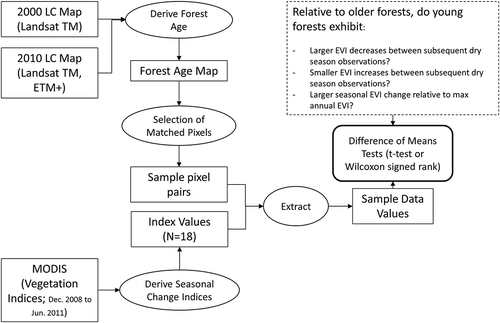
Further investigation into the role of stand age in determining temporal patterns and intensity of forest deciduousness is required to identify the drivers of deciduousness during relatively dry years, when this behavior is substantially more prevalent than it is in wet years (Cuba et al. 2013). Analysis of the drivers of leaf drop during dry years indicates potential future forest behavior under a broader range of climatic conditions (Costa et al. 2007; Salazar, Nobre, and Oyama 2007). This paper distinguishes young forest stands from older stands at regional scales using land-cover maps from 2000 and 2010, and uses matched-pairs statistical tests to examine differences in the timing and intensity of deciduousness across forest age classes for three dry seasons during the years 2008–2011 (Figure 1).

Figure 1. Flowchart depicting methodology of the analysis.

2. Methods

2.1. Study area

The seasonally dry tropical forests of the southern Yucatán are the largest remaining forest tracts in Mexico and are subject to competing tensions of forest conservation, cattle pasture use, and small-scale swidden cultivation (Turner et al. 2001). Despite political, economic, and environmental pressures related to globalization, government-sponsored development, and climate in the region, the traditional maize-based milpa cultivation land use persists in the region (Schmook et al. 2013) and the rate of crop-fallow cycles has intensified (Schmook 2010). Rates of deforestation have declined in recent decades (Rueda 2010) from the high rates seen in the 1970s and 1980s (Klepeis and Turner 2001), but regional forests remain vulnerable to a range of disturbances including hurricanes, wild fires, and drought (Cheng et al. 2013; Márdero et al. 2012; Rogan et al. 2011). The study area covers approximately 18,000 km² in the states of Campeche and Quintana Roo, encompassing the Calakmul Biosphere Reserve, and is dominated by deciduous and non-deciduous forests (Figure 1). Forest types in the region have been distinguished on the basis of tree stature, tendency to exhibit deciduousness, and exposure to seasonal flooding (Pérez-Salicrup 2004; Schmook et al. 2011). The regional mean annual temperature is 27°C, and mean precipitation ranges approximately 750–1400 mm/year (Neeti et al. 2012). Rainfall exhibits a seasonal pattern, with a wet season that typically runs from June to October and a dry season from November to May (Magaña, Amador, and Medina 1999).

The extent and intensity of dry season deciduousness in the study area exhibit high interannual variability, with extreme deciduousness associated with seasonal conditions of high temperature and low precipitation. Deciduousness is most frequent and intense across years in the northwest of the study area, although relatively wet forests in the central part of the study area may exhibit facultative deciduousness during dry season months of atypically hot and dry conditions (Cuba et al. 2013).

2.2. Measuring deciduousness

Phenological patterns were observed and parameterized through the use of metrics derived from MODIS Vegetation Index image series for June 2008 to May 2011, a 36-month period divisible into three annual periods beginning DOY 153 each of which completely contains the duration of the dry season, as well as conditions of peak greenness that precede the dry season. This three year period is chosen because it contains the date of the most recent land-cover map (2010), and describes interannual phenological variability by monitoring behavior across multiple dry seasons. The MOD13Q1 product is a 16-day composite of MODIS data from the Terra platform distributed at 250 m spatial resolution and contains vegetation index, quality, reflectance, and viewing angle information (Solano et al. 2010). Marginal quality pixel values or instances of infilled missing data, as revealed in the product quality layer, were excluded from analysis.

The Enhanced Vegetation Index (EVI) was used, calculated as Equation (1), where “NIR,” “Red,” and “Blue” refer to reflectance in the near-infrared, red, and blue bands, respectively (Huete et al. 2002):

(1)

Vegetation indices such as EVI have long been fundamental to remote-sensing studies of phenology as measure of surface properties, such as vegetation productivity and canopy structure (de Beurs and Henebry 2010; Morisette et al. 2009). Compared with other vegetation indices such as NDVI, EVI uses blue band reflectance to measure aerosols and limit the attenuation and scattering effect on observed reflectance in the red band, and is insensitive to saturation, offering high sensitivity to differences in canopy structure and content in areas of dense tropical vegetation (Huete et al. 2002) such as the Mexican Yucatán.

In order to allow for a sufficient number of good quality observations during each time period examined, pairs of consecutive 16-day MODIS composites from the dry season were combined into maximum value composites that cover a 32-day period. Six such 32-day periods in each of three dry seasons were covered in this way, with start dates of DOY 337, DOY 001, DOY 033, DOY 065, DOY 097, and DOY 129. In order to refer to a specific 32-day compositing period, this study uses brackets around the start day of year for that period, e.g., “the period [033].” The use of quasi-monthly temporal compositing periods also allows for easier comparison of results to the monthly field measurements made by Lawrence (2005).

Normalized change of EVI (Equation (2)) at a given time (t_n) with respect to the initial dry season value (t₀; i.e. that observed in the [337] period, or the [001] period for a small portion of pixels in the 2009–2010 dry season) was measured five times in each of three study years, producing a total of 15 temporal metrics (Frazier et al. 2014) related to the seasonal intensity of deciduousness for each pixel at different times during the dry season, for the periods DOY 001–032, 033–064, 065–096, 097–128, and 129–152. In addition to these temporal metrics, for each study year the normalized seasonal change in EVI, defined as the observed annual range of EVI divided by the observed annual maximum EVI (Cuba et al. 2013), was measured to describe the overall intensity of deciduousness. Each of these 18 metrics was then extracted at sample forest pixels of different age and the significance of observed differences was assessed.

(2)

MODIS data were used to track forest phenology within the study area, yet regional and continental scale classification of dry tropical forest using MODIS data suggest that fine or moderate resolution data can effectively capture the scale and spectral signature of landscape heterogeneity (Batholome et al. 2002; Kalaczka et al. 2008; Miles et al. 2006; Sánchez-Azofeifa and Portillo-Quintero 2011). In order to limit difficulties related to fine-scale land-cover heterogeneity and classification confusion, forest age classes were derived from Landsat 30 m land-cover data and then upscaled to correspond to the 250 m MODIS data using category abundance thresholding approach described in Section 2.4.

2.3. Estimating forest age

Two closed-canopy, upland forest age classes (12–22 years, and >22 years) were identified from an overlay analysis of two Landsat-based 30 m land-cover maps from years 2000 and 2010, grouping forest pixels by their age in year 2010. Forest pixels were further differentiated on the basis of whether or not seasonal deciduousness was a typical response of the vegetation, exhibited annually. This subsection details each of the maps used, and summarizes the procedure through which forest age was deduced.

The 2000 map was produced using a step-wise In-Process Classification Assessment (IPCA) method, and is comprehensively summarized by Schmook et al. (2011). The set of 14 land-cover categories in the map includes three categories of secondary vegetation (herbaceous, shrubby, and arboreous), two categories of non-deciduous upland forest, and one category of deciduous forest. Schmook et al. (2011) classified vegetation younger than 12 years as secondary based on field observation, with older vegetation classified as forest. Overall accuracy of the map is 87%, while user’s accuracies for individual forest and secondary categories range from 64% (upland semi-deciduous forest) to 97% (herbaceous secondary). This degree of precision in categorizing vegetation age ranges, and rates of classification accuracy, are in line with summary findings of results typical from Landsat-based analysis (see Fujiki et al. 2016).

The 2010 map was produced from this analysis using a hybrid supervised/unsupervised, iterative approach similar to the IPCA method used for the 2000 map (see Schmook et al. 2011), using ground reference data and aerial imagery (Franklin et al. 2003). The map is based on spectral data from two Landsat-5 TM images acquired on 26 January 2010 and four Landsat-7 ETM+ images acquired on 2 January 2010, 11 January 2010, 28 February 2010, and 8 September 2010. Unsupervised clustering was used to stratify data into four broad categories of mature forest, young/low-stature vegetation, semi-aquatic vegetation, and agriculture. For the semi-aquatic vegetation and agriculture strata, self-organizing cluster analysis (Ball and Hall 1965) was used to identify nine information categories. For the forest and young vegetation strata, Classification Tree Analysis was used to allocate pixels to one of seven categories. The final set of 16 categories includes one category of secondary vegetation, three categories of non-deciduous upland forest, and one category of deciduous forest. Overall accuracy of the map based on ground reference data from field visits is 86%, while user’s accuracies for individual forest and secondary categories range from 71% for Selva baja (i.e., wetland-upland transition forests) to 100% for Subcaducafolia (i.e., low and medium stature, semi-deciduous upland forests).

Prior to map comparison, categories in both land-cover maps were aggregated to one of four broad categories: Secondary Vegetation, Non-Deciduous Forest, Deciduous Forest (Table 1), as well as an additional Other category that was omitted from further analysis. Aggregation resulted in higher category-level user’s and producer’s accuracies, due to the elimination of classification errors involving similar forest or secondary categories that were combined in the process of aggregation. Due to differences of categorical separability in the classification processes that resulted in textural dissimilarities in the maps, a 5 × 5 mode filter was used on the year 2000 post-aggregation land-cover map to remove fine-scale categorical variability and yield a map with texture that corresponded closely to that of the year 2010 map. The aggregated, four-category land-cover maps were overlaid and the resulting image contained six cross-tabulation categories of interest: two which describe growth of secondary vegetation to forest, two which describe persistence of forest, and two which describe areas classified as deciduous forest in one map but non-deciduous forest in the other. The remaining 10 cross-tabulation categories described disturbance events, persistence of non-forest land-cover, or involved the Other category in one or both years and so were omitted from the analysis. The two categories of interest in which pixels were classified as deciduous forest in one map but non-deciduous forest in the other do not represent areas of actual land-cover change but rather areas exhibiting interannual variability in deciduous phenology, and are referred to as semi-deciduous because they are observed to exhibit deciduousness in only one of the two years for which maps were available. Pixels in each of the four other analyzed categories are considered typically deciduous, or non-deciduous, according to the forest type to which they were classified in at least one of the 2000 and 2010 land-cover maps.

Table 1. Three aggregated secondary and non-deciduous forest land-cover categories were used to standardize the 2000 and 2010 land-cover maps prior to analysis. While Selva Baja transition forests were included in the aggregate Non-Deciduous Forest category, seasonally inundated Bajos were excluded.

	Secondary	Deciduous forest	Non-deciduous forest
2000	Herbaceous secondary (1–2 years of regrowth)	Low- and medium- staturesemi-deciduous upland forest	Medium-stature semi-evergreen upland forest
	Shrubby secondary (3–6 years of regrowth)		Tall-stature evergreen upland forest
	Arboreous secondary (7–12 years of regrowth)
User’s accuracy	0.96	0.64	0.92
Producer’s accuracy	0.84	0.98	0.94
2010	Secondary	Subcaducafolia	Selva Alta/Mediana
			Selva Baja
			Selva Mediana
User’s accuracy	0.81	1	1
Producer’s accuracy	0.81	0.84	0.78

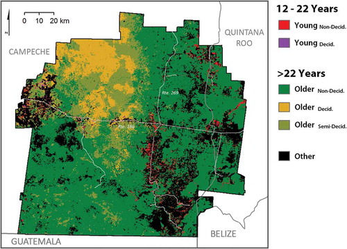
Forest stand age was assigned for all pixels classified as forest in 2010 based on observed land-cover change or persistence involving one or more secondary or mature forest category. In each of the 2000 and 2010 maps, pixels of secondary vegetation categories contained all vegetation younger than 12 years (after Schmook et al. 2011), while pixels of forest categories contained vegetation older than 12 years. Subtracting this parameter from the dates of the land-cover maps allowed estimation of the earliest and latest possible dates of forest conversion for each of the six cross-tabulation categories of interest. Forest pixels were allocated to one of two age classes: young forest (12–22 years) if the pixel was classified as secondary in 2000 and forest in 2010; and older forest (>22 years) if the pixel was classified as forest in both 2000 and 2010 (Table 2).

Table 2. Forest age was derived from land-cover maps of years 2000 and 2010, assuming vegetation aged less than 12 years would be classified as secondary, and vegetation aged more than 12 years would be classified as forest.

Age class	Age in year 2010 (years)	Land cover in 2000		Land cover in 2010		Earliest possible year of conversion	Latest possible year of conversion
Young Deciduous	12–22	Secondary		Non-deciduous forest		1988	2008
Young Non-Deciduous	12–22	Secondary		Deciduous forest		1988	2008
Older Non-Deciduous	> 22	Non-deciduous forest		Non-deciduous forest		–	1988
Older Deciduous	> 22	Deciduous forest		Deciduous forest		–	1988
		Non-deciduous forest		Deciduous forest
Older Semi-deciduous	> 22		OR			–	1988
		Deciduous forest		Non-deciduous forest

The map of forest age was upscaled from a spatial resolution of 30 m to 250 m to approximate the spatial resolution of the MOD13Q1 data, facilitating the extraction of phenological metrics from EVI time series. The dominant land-cover change vector in the study area is conversion of forest or secondary forest for croplands or pasture, in patches on the order of 1–5 ha in size (Vester et al. 2007). This process creates a heterogeneous landscape pattern of forest age, and taking several 30 m pixels together to create a MODIS-sized pixel can result in pixels of mixed land use and forest age at this coarser scale. In order to select the 250 m pixels that were most homogenous with respect to forest age, a relative abundance threshold was used to filter out pixels of heterogeneous land cover when upscaling. This thresholding technique designated coarse 250 m pixels to a homogeneous age class only if at least 90% of the Landsat pixels within their footprint was comprised of a single age class; otherwise, they were considered too heterogeneous to be used to extract representative, phenological trends.

2.4. Sampling method

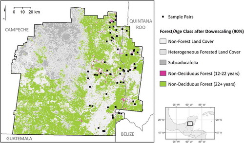
Older, non-deciduous forest pixels were of relatively homogeneous composition compared to young forest pixels (Figure 3), and sample pairs were determined by initially selecting a homogeneous pixel from the young forest age class. When upscaling forest age data from medium to coarse spatial resolution, using a 90% scaling threshold to filter potential sampling sites in both maps yielded 599 total pixels of young non-deciduous forest that were homogeneous with respect to land cover. If textural filtering had not been implemented in the map of year 2000, then different threshold values for each map would be appropriate. A substantial portion of these pixels were located within 1.5 km of homogeneous older non-deciduous forest, yielding 261 possible sample pairs. Threshold values of pixel land-cover homogeneity that were higher than 90% decreased the number of viable sample pixels of young forest and did not allow for sufficient sample pairs when using the 1.5 km maximum distance threshold. At least one sample distribution was observed to be significantly non-normal for 14 of the 18 metrics, and thus four matched-pairs t-tests and 14 Wilcoxon signed rank tests were used to test for significant differences between the young and older forest classes.

Figure 2. Study area in the southern Yucatán, Mexico (2010 land-cover data shown).

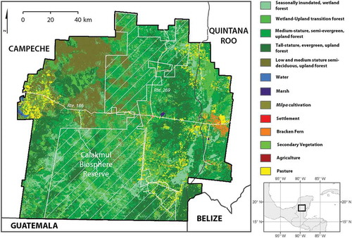
Figure 3. Forest age classes were derived from year 2000 and year 2010 land-cover maps in the study area, for all pixels of forest persistence and all pixels of change from secondary vegetation to forest.

2.5. Statistical tests of difference

Statistical tests were used to detect significant differences in EVI-based phenological metrics between young and older forests. Shapiro–Wilk tests of normality were performed for each sample and each metric to determine the appropriate test. Matched-pairs t-tests were used for comparisons in which both samples exhibited normal distributions, and Wilcoxon signed rank tests were used in instances where at least one sample distribution was observed to be non-normal at 95% confidence. Both matched-pairs t-tests and Wilcoxon signed rank tests rely on samples of matched pairs to examine whether discrete treatments or specific discrepancies explain observed differences between groups, and have been employed in studies of disease (Jewell 2004), ecosystem restoration (Benayas et al. 2009), and eco-certification programs (Rueda and Lambin 2013).

Randomly sampled pixels from the young forest age class (12–22 years) were each matched to a pixel from the older forest age class (>22 years) located within 1.5 km to constitute a matched pair. The initial pixel of a sample pair was selected from the young forest age class because of its relatively limited spatial extent relative to the abundant older forest age class. The 1.5 km maximum distance threshold was high enough to allow for a sufficiently high number of potential candidate pairs, while low enough to ensure that paired pixels exhibit some degree of similarity with respect to soil type, elevation, precipitation, and temperature, so that differences in phenological metrics related to the timing and intensity of deciduousness could be attributed to forest age.

A comparison was performed to test the statistical significance of observed differences with respect to six phenological metrics in each of three years between young and older forest pixels that were typically non-deciduous. Forests normally designated as non-deciduous were selected to exclude forests that predictably shed all or a large portion of their canopy every year (see Cuba et al. 2013). Although the forest types that were sampled do not typically shed a large portion of their leaves during the dry season in all years, they may exhibit facultative deciduousness in some years in response to drought conditions, and thus exhibit potentially greater interannual behavioral variability of deciduous phenology. Furthermore, an increase in deciduous behavior in these typically non-deciduous forests would constitute evidence for a climatic shift, either short term or long term. Thus, deciduousness in typically non-deciduous forests is useful as an indicator of ecosystem response to future climate changes. Finally, the likelihood of comparing forest stands of truly different age was higher: our ability to define forest age was greater as the user’s accuracies in the 2000 land-cover map were substantially higher for non-deciduous forest (92%) than for deciduous forest (64%).

3. Results

3.1. Forest age

Forest age was calculated for all pixels exhibiting persistence of forest or change from secondary vegetation to forest (Figure 2). This area amounted to 83.7% of the total study area, or approximately 274,000 of 328 000,pixels, while the remaining portion of the study area did not exhibit persistence of, or change between, secondary and mature forest categories. Non-deciduous forest was the most extensive forest type (61.7% of total study area), followed by semi-deciduous forest (11.5%) and deciduous forest (10.5%). Older forest, aged 22 or more years, was the most extensive forest age class (78.9%), while young forest (12–22 years) comprises a much smaller portion of the study area (2.2%). Young forest was concentrated in locations of forest conversion to agriculture and pasture use, including the relatively accessible corridors along Rtes. 186 and 269 that run through the study area east-to-west and north-to-south, respectively. The deciduous forest and semi-deciduous forest classes comprised much of the northwest quarter of the study area, with non-deciduous forest classes being predominant in the south and east.

3.2. Statistical tests of phenological difference

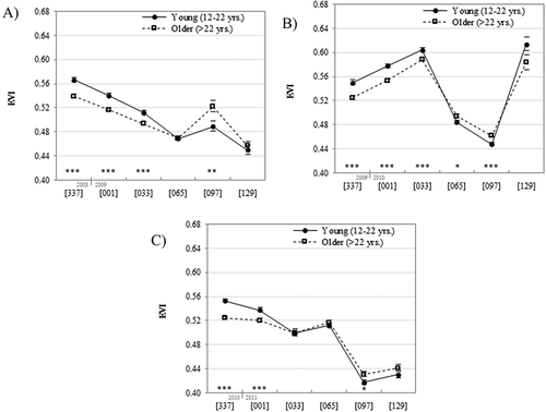
Each of three dry season temporal profiles is comprised of pixel-maximum EVI observations made over six 32-day periods, for both young (12–22 years) and older (>22 years) forests, averaged over the portion of the sample where good quality observations were available for both pixels in a matched pair (Figure 4). Temporal profiles of the sample mean EVI for the dry season periods (i.e. the periods beginning DOY 337 to DOY 129) in each of the three years revealed substantial interannual variability in forest phenology for all forest age classes, as well as significant differences between young and older forest pixels that comprised the matched pair sample. Averaged for all periods per year, EVI for young and older forests, respectively, was 0.504 and 0.500 in 2008–2009; 0.546 and 0.534 in 2009–2010; and 0.492 and 0.489 in 2010–2011. In all three dry seasons, the young forest sample had a significantly (p < 0.001) higher average EVI than the older forest sample during the early dry season periods [337] and [001]. In contrast, in all dry seasons, the average maximum EVI was lower for the young forest than for older forest in the late dry season period [097] (for all years, p < 0.02). A general downward temporal trend in EVI was seen during the 2008–2009 dry season, with an increase in period [097]. The 2010–2011 dry season was also characterized by broad decline in EVI, although much of the seasonal difference is between periods [065] and [097]. In contrast, the temporal pattern of EVI in the 2009–2010 dry season showed early increases in EVI, followed by two periods of relatively low EVI before an increase seen in period [129] (Figure 4).

Figure 4. The locations of sample pairs for the three comparisons of young and older forest classes are shown. Outlines have been added around the young forest age class to enhance interpretation.

Tests involving the set of temporal phenological metrics measuring normalized seasonal EVI change over total annual periods and in successive 32-day periods during the dry season revealed substantial significant differences between matched pair samples of young and older forests (Figure 5; Table 3). A total of 14 of the 15 comparisons of normalized EVI change during the dry season revealed significantly different (p < 0.05) magnitudes of normalized change between the young forest pixels and the older forest pixels. For all 14 instances of significantly different normalized change, younger forests exhibited values less than those of more mature forests: 11 were cases where the normalized decline in average EVI of young forests was greater than that of older forests, 3 were cases where the normalized increase in average EVI of young forests was less than that of older forests.

Table 3. Results of matched-pair t-tests (non-italicized) and Wilcoxon signed rank tests (italicized) for matched pair samples of young (12–22 years) and older (>22 years) forests, with respect to 18 phenological metrics.

	µ Young(12–22 years)	µ Older (>22 years)	N	p-Value
EVI normalized seasonal change (total year)
2008.153 to 2009.152	0.329	0.293	260	<0.001
2009.153 to 2010.152	0.342	0.301	260	<0.001
2010.153 to 2011.152	0.395	0.350	260	<0.001
EVI normalized change measured in successive 32-day periods
2008–2009 dry season
[337] to [001]	−0.044	−0.042	254	0.35
… to [033]	−0.096	−0.080	260	0.02
… to [065]	−0.174	−0.130	240	<0.001
… to [097]	−0.136	−0.032	91	<0.001
… to [129]	−0.177	−0.132	81	<0.001
2009–2010 dry season
[337] to [001]	+0.064	+0.089	68	0.01
… to [033]	+0.053	+0.089	260	<0.001
… to [065]	−0.158	−0.086	251	<0.001
… to [097]	−0.217	−0.144	232	<0.001
… to [129]	+0.029	+0.087	31	0.02
2010–2011 dry season
[337] to [001]	−0.025	−0.007	259	<0.001
… to [033]	−0.096	−0.050	96	<0.001
… to [065]	−0.070	−0.012	259	<0.001
… to [097]	−0.244	−0.175	211	<0.001
… to [129]	−0.218	−0.160	179	<0.001

Figure 5. Temporal profiles of average maximum EVI values for young and older forest samples over 32-day periods during the 2008–2009 (a), 2009–2010 (b), and 2010–2011 (c) dry seasons. Asterisks denote significant differences by forest age class (*: p < 0.05; **: p < 0.01; ***: p < 0.001). Bars mark one standard error above and below sample mean.

Young forests had significantly higher normalized seasonal EVI change than older forests in each of the three annual periods (p < 0.001). These differences indicate that young forests exhibited a greater range of seasonal EVI change relative to maximum EVI than older forests, with differences equal to: 0.036 in the annual period 2008–2009; 0.041 in the annual period 2009–2010; and 0.046 in the annual period 2010–2011. Interannual variability of normalized seasonal EVI change was comparable to the difference observed between forest age classes: the young forest sample mean increased 0.014 from the 2008–2009 annual period to the 2009–2010 annual period, and 0.0528 from the 2009–2010 annual period to the 2010–2011 annual period; while the older forest sample mean increased 0.008 from the 2008–2009 annual period to the 2009–2010 annual period, and 0.0486 from the 2009–2010 annual period to the 2010–2011 annual period.

4. Discussion

The comparison of young (12–22 years) and older (>22 years) forests with respect to EVI-derived phenological metrics presents strong evidence that young forest stands exhibit different patterns of deciduous phenology from older forest. The nature of the temporal differences: with all 14 significant (p < 0.05) cases being instances of EVI declining more, or increasing less, relative to an initial early dry season value for younger forest than older forest, suggests that younger forests are more likely to exhibit deciduousness during water-limited periods than older forests. Since a maximum distance of 1.5 km is used to match sample pixels from different age classes, observed differences in deciduous phenology can be attributed to forest stand age rather than environmental factors such as soil type, elevation, precipitation, and vapor pressure deficit that exhibit considerably higher variability at regional spatial scales.

The Lawrence (2005) study that measured litterfall from 1998 to 2000 revealed that a large portion of total annual litterfall mass was collected in the dry season months of February, March, and April. This time interval of DOY 032 to 120 corresponds most closely to the dates covered by the third, fourth, and fifth 32-day periods used in this analysis: [033], [065], and [097]. The high interannual variability in the magnitude and direction of normalized EVI change measured during these three late dry season 32-day periods is notable, with higher EVI observed in period [097] than in period [065] in 2009, and in period [065] compared to period [033] in 2011. Despite this variability, significant differences in EVI change are observed in five of the six change intervals defined by these nine periods, with all five being cases where young forest showing larger normalized EVI declines than those of older forest (Table 3).

However, evaluation of these results against the findings of Lawrence (2005) is limited by the ways in which deciduousness is measured differently using remotely sensed data than it is using plot-based ground methods. Lawrence (2005) measured the monthly amount of litterfall mass collected in four traps at 36 plots, distributed across 3 sites, over a 15-month period. A large portion of litter could be attributed to deciduous leaf shedding during periods of drought stress, predominantly occurring in dry season months, but the total mass of litterfall also potentially includes leaves and stems removed during rainy season storms or lost because of tree mortality. Multispectral satellite sensors offer direct observation of the canopy and can monitor changes in canopy structure over time, but are unable to measure relatively low amounts of leaf loss during the wet season with high precision (Glenn et al. 2008; Castillo et al. 2012). The other fundamental difference between the two approaches is that litter traps do not measure the amount or proportion of leaves remaining on the trees. If deciduousness is considered a measurement which incorporates both leaf litterfall and canopy bareness, differences between observations from the ground and remote sensing observations are more easily resolved.

The normalized seasonal change of EVI is one metric designed to correspond to the observational capacities of multispectral remote sensing of the canopy. In all three annual periods from June 2008 to May 2011, the young forest age class exhibits a significantly higher normalized seasonal change of EVI. Lawrence (2005) found that the mass of litterfall as well as the coefficient of variation of litterfall (or the intensity of seasonality) increased significantly with forest age. These results might suggest more intense deciduousness in older forests than in younger stands. However, in the absence of information on how much of the canopy remains covered with leaves, deciduousness measured as the portion of total leaves shed seasonally cannot be assessed. The logarithmic function that defines the increase in litterfall with forest age (Lawrence 2005) indicates decreasing marginal litterfall with increasing age, and increasing canopy leaf area. For all years 2008–2011, the normalized seasonal change of EVI comparisons in this paper suggest younger forest stands, with lower total leaf area than older forest stands, are more likely to exhibit higher intensity deciduousness than older forest, behavior that would be expected based on observations from the 1998–2000 ground data (Lawrence 2005).

The higher normalized seasonal change of EVI observed for the younger forest class compared to the older forest class is a consequence of younger forests exhibiting higher maximum annual EVI values as well as lower minimum EVI values. While the total leaf area of younger forests is expected to be lower than that of older forests, forest stands at 12–22 years will have a closed canopy and stature approaching that of stands of similar forest type at age greater than 22 years. Higher maximum EVI in younger forests might be attributable to biophysical properties such as leaf age and health, structure of the canopy, or to differential amounts of shade. This relationship is the same observed by a comparison of average annual EVI values in subtropical semi-deciduous natural forest and in deciduous plantation forests in southern China (Kou et al. 2015). After an initial period of 4–5 years after forest conversion during which plantation EVI values are lower than in the forest land-cover present before conversion, young plantations have higher average annual EVI, as well as higher maximum EVI and lower minimum EVI values, compared to natural forest (Kou et al. 2015). Galvao et al. (2016) find that MODIS EVI values in subtropical deciduous forests that are uncorrected for topography and incidence angle are up to 15% greater than corrected values over sunlit surfaces, yet up to 47% less than corrected values over shaded surfaces. Although younger forest stands are closed canopy, due to their limited age they will lack older, taller, dominant trees found in mature forest. Such dominant trees can cast shadow on other tree crowns of lower height, increasing the proportion of shaded top-of-canopy relative to younger forest. Such as increased shade portion may explain the lower observed maximum EVI values in older forests compared to values in younger forests that are more homogenous with respect to tree height. Lower minimum EVI in younger forests might be attributable to a smaller amount of non-deciduous understory vegetation and lianas, as well as more intense dry season deciduous leaf loss from the canopy.

The finding that young forests exhibit dry season deciduousness significantly more intensely than older forests suggests the potential for increased vulnerability of dry tropical forests to atypically hot and dry climate conditions beyond the land systems of the southern Yucatán. Global trends of decelerating tropical deforestation, coupled with forest regrowth and ecosystem restoration efforts (Aide et al. 2012; Meyfroidt and Lambin 2011), yield a younger average age of forest, and a large extent of forest at relatively early successional stages. Significant differences in the phenology of these forests may impact ecosystem functioning in terms of local floral and faunal species assemblages, fuel loads, and nutrient availability (Condit et al. 2000; DeLonge, D’Odorico, and Lawrence 2008; van der Werf et al. 2010).

Beyond their relevance to predictions of future forest condition, the methods employed in this study may have utility to forest monitoring efforts. Regional assessments of forest AGB and carbon density for use in estimates of greenhouse gas emissions from deforestation are challenged by the spectral similarity of intermediate-age and older forests, despite large differences in the AGB between forests of different age (Baccini et al. 2012; Goetz et al. 2009; versus e.g. Read and Lawrence 2003). Field data collections and active remote-sensing instruments have been used to constrain forest AGB and carbon density at fine spatial scales and provide parameters to be scaled or interpolated (Asner et al. 2010; Lefsky et al. 2005), but future exploration of phenological differences attributable to forest age may offer innovative alternative methods for AGB and carbon stock assessment. Future work may also investigate the potential effect on phenology of repeat clearing of vegetation for agricultural use (Lawrence et al. 2007; Schmook 2010), examine a greater number of forest age classes, or better constrain the relationship between remotely sensed indicators of deciduousness and the amount and timing of litterfall measured at field plots.

5. Conclusion

Forest age was derived for dry tropical forests in the southern Yucatán Peninsula, and time series of MODIS EVI data were used to describe deciduous phenology over a 36-month period 2008–2011. Matched-pairs statistical tests revealed significant differences in deciduous phenology between young (12–22 years) and older (> 22 years) forest stands of different age classes during the dry season. Accounting for variability in soil type and weather conditions, older forest (>22 years) exhibited significantly lower normalized seasonal EVI change than young (12–22 years) forests, suggestive of less prevalent or intense deciduous leaf loss due to the deeper root systems or greater water storage capacity of trees in older forest stands. With respect to normalized EVI change relative to start-of-dry-season values, measured at successive 32-day periods during the dry season, 14 of 15 measurements showed significant (p < 0.05) differences between young and older forests, and in all cases young forest EVI declined more, or gained less, than older forest EVI.

Acknowledgment

The authors thank J. Ronald Eastman, Bryan Pijanowski, Laura Schneider, and B.L. Turner II for their comments on the work, as well as anonymous reviewers.

Disclosure statement

No potential conflict of interest was reported by the authors.

Additional information

Funding

This work was supported by NASA Headquarters under the NASA Earth and Space Science Fellowship Program – [Grant NNX12AO04H S01], and the Gordon and Betty Moore Foundation under grant [#1697].

References

- Aide, T. M., M. L. Clark, H. R. Grau, D. López-Carr, M. A. Levy, D. Redo, M. Bonilla-Moheno, G. Riner, M. J. Andrade-Núñez, and M. Muñiz. 2012. “Deforestation and Reforestation of Latin America and the Caribbean (2001–2010).” Biotropica 45: 262–271. doi:10.1111/j.1744-7429.2012.00908.x.
- Asner, G. P., G. V. N. Powell, J. Mascaro, D. E. Knapp, J. K. Clark, J. Jacobson, T. Kennedy-Bowdoin, et al. 2010. “High-Resolution Forest Carbon Stocks and Emissions in the Amazon.” Proceedings of the National Academy of Sciences of the USA 107: 16738–16742. doi:10.1073/pnas.1004875107.
- Baccini, A., S. J. Goetz, W. S. Walker, N. T. Laporte, M. Sun, D. Sulla-Menashe, J. Hackler, et al. 2012. “Estimated Carbon Dioxide Emissions from Tropical Deforestation Improved by Carbon-Density Maps.” Nature Climate Change 2: 182–185. doi:10.1038/nclimate1354.
- Ball, G. H., and D. J. Hall. 1965. A Novel Method of Data Analysis and Pattern Classification. Menlo Park, CA: Stanford Research Institute.
- Batholome, E., A. S. Belward, F. Achard, S. Bartalev, C. Carmona-Moreno, H. Eva, S. Fritz, J. Gregoire, P. Mayaux, and H. J. Stibig. 2002. GLC 2000 – Global Land Cover Mapping for the Year 2000 – Project Status November 2002, EUR 20524 EN. Luxembourg: Publication of the European Commission.
- Benayas, J. M. R., A. C. Newton, A. Diaz, and J. M. Bullock. 2009. “Enhancement of Biodiversity and Ecosystem Services by Ecological Restoration: A Meta-Analysis.” Science 325: 1121–1124. doi:10.1126/science.1172460.
- Bohlman, S. A. 2010. “Landscape Patterns and Environmental Controls of Deciduousness in Forests of Central Panama.” Global Ecology and Biodiversity 19: 376–385. doi:10.1111/j.1466-8238.2009.00518.x.
- Castillo, M., B. Rivard, G. A. Sánchez-Azofeifa, J. Calvo-Alvarado, and R. Dubayah. 2012. “LIDAR Remote Sensing for Secondary Tropical Dry Forest Identification.” Remote Sensing of Environment 121: 132–143. doi:10.1016/j.rse.2012.01.012.
- Cheng, D., J. Rogan, L. Schneider, and M. Cochrane. 2013. “Evaluating MODIS Active Fire Products in Subtropical Yucatán Forest.” Remote Sensing Letters 4: 455–464. doi:10.1080/2150704x.2012.749360.
- Condit, R., K. Watts, S. Bohlman, R. Pérez, R. B. Foster, and S. P. Hubbell. 2000. “Quantifying the Deciduousness of Tropical Forest Canopies under Varying Climates.” Journal of Vegetation Science 11: 649–658. doi:10.2307/3236572.
- Costa, M. H., S. N. M. Yanagi, P. Souza, A. Ribeiro, and E. J. P. Rocha. 2007. “Climate Change in Amazonia Caused by Soybean Cropland Expansion, as Compared to Change Caused by Pastureland Expansion.” Geophysical Research Letters 34: L07706. doi:10.1029/2007GL029271.
- Crist, E. P., and R. C. Cicone. 1984. “A Physically-Based Transformation of Thematic Mapper Data-The TM Tasseled Cap.” IEEE Transactions on Geoscience and Remote Sensing 22: 256–263. doi:10.1109/tgrs.1984.350619.
- Cuba, N., J. Rogan, Z. Christman, C. A. Williams, L. C. Schneider, D. Lawrence, and M. Millones. 2013. “Modeling Dry Season Deciduousness in Mexican Yucatán Forest Using MODIS EVI Data (2000–2011).” GIScience & Remote Sensing 50: 26–49. doi:10.1080/15481603.2013.778559.
- de Beurs, K. M., and G. M. Henebry. 2010. “Spatio-Temporal Statistical Methods for Modeling Land Surface Phenology.” In Phenological Research: Methods for Environmental and Climate Change Analysis, edited by I. L. Hudson and M. R. Keatley, 177–208. Dordrecht, Netherlands: Springer.
- DeLonge, M., P. D’Odorico, and D. Lawrence. 2008. “Feedbacks between Phosphorus Deposition and Canopy Cover: The Emergence of Multiple Stable States in Tropical Dry Forests.” Global Change Biology 14: 154–160. doi:10.1111/j.1365-2486.2007.01470.x.
- Franklin, J., S. R. Phinn, C. E. Woodcock, and J. Rogan. 2003. “Rationale and Conceptual Framework for Classification Approaches to Assess Forest Resources and Properties.” In Methods and Applications for Remote Sensing of Forests: Concepts and Case Studies, edited by M. Wulder and S. E. Franklin, 279–300. Dordrecht, Netherlands: Kluwer.
- Frazier, R., N. C. Coops, M. A. Wulder, and R. Kennedy. 2014. “Characterization of Aboveground Biomass in an Unmanaged Boreal Forest Using Landsat Temporal Segmentation Metrics.” ISPRS Journal of Photogrammetry and Remote Sensing 92: 137–146. doi:10.3390/s8042136.
- Fujiki, S., K. Okada, S. Nishio, and K. Kitayama. 2016. “Estimation Of The Stand Ages Of Tropical Secondary Forests After Shifting Cultivation Based On The Combination Of Worldview-2 And Time-series Landsat Images.isprs Journal Of Photogrammetry And Remote Sensing.” 119: 280-293. doi: 10.1016/j.isprsjprs.2016.06.008.
- Galvão, L. S., F. M. Breunig, T. S. Teles, W. Gaida, and R. Balbinot. 2016. “Investigation Of Terrain Illumination Effects On Vegetation Indices And Vi Derived Phenological Metrics In Subtropical Deciduous Forests.” Giscience & Remote Sensing 53 69–381: 53 69-381. doi: 10.1080/15481603.2015.1134140.
- Giraldo, J. P., and N. M. Holbrook. 2011. “Physiological Mechanisms Underlying the Seasonality of Leaf Senescence and Renewal in Seasonally Dry Tropical Forest Trees.” In Seasonally Dry Tropical Forests: Ecology and Conservation, edited by R. Dirzo, H. S. Young, H. A. Mooney, and G. Ceballos, 129–140. Washington: Island Press.
- Glenn, E. P., A. R. Huete, P. L. Nagler, and S. G. Nelson. 2008. “Relationship between Remotely-Sensed Vegetation Indices, Canopy Attributes, and Plant Physiological Processes: What Vegetation Indices Can and Cannot Tell Us about the Landscape.” Sensors 8: 2136–2160. doi:10.3390/s8042136.
- Goetz, S. J., A. Baccini, N. T. Laporte, T. Johns, W. Walker, J. Kellndorfer, R. A. Houghton, and M. Sun. 2009. “Mapping and Monitoring Carbon Stocks with Satellite Observations: A Comparison of Methods.” Carbon Balance and Management 4: 2. doi:10.1186/1750-0680-4-2.
- Huete, A. R., K. Didan, T. Muira, E. P. Rodriguez, X. Gao, and L. G. Ferreira. 2002. “Overview of the Radiometric and Biophysical Performance of the MODIS Vegetation Indices.” Remote Sensing of Environment 83: 195–213. doi:10.1016/s0034-4257(02)00096-2.
- Jaramillo, V. J., A. Martínez-Yrízar, and R. L. Sanford Jr. 2011. “Primary Productivity and Biogeochemistry of Seasonally Dry Tropical Forests.” In Seasonally Dry Tropical Forests: Ecology and Conservation, edited by R. Dirzo, H. S. Young, H. A. Mooney, and G. Ceballos, 109–128. Washington: Island Press.
- Jewell, N. P. 2004. Statistics for Epidemiology. Boca Raton: Chapman and Hall/CRC.
- Kalacska, M., G. A. Sánchez-Azofeifa, J. C. Calvo-Alvarado, G. A. Rivard, and M. Quesada. 2005b. “Effects of Season and Successional Stage on Leaf Area Index and Spectral Indices in Three Mesoamerican Tropical Dry Forests.” Biotropica 37: 486–496. doi:10.1111/j.1744-7429.2005.00067.x.
- Kalacska, M., J. C. Calvo-Alvarado, and G. A. Sánchez-Azofeifa. 2005a. “Calibration and Assessment of Seasonal Changes in Leaf Area Index of a Tropical Dry Forest in Different Stages of Succession.” Tree Physiology 25: 733–744. doi:10.1093/treephys/25.6.733.
- Kalaczka, M., G. A. Sánchez-Azofeifa, B. Rivard, J. C. Calvo-Alvarado, and M. Quesada. 2008. “Baseline Assessment for Environmental Services Payments from Satellite Imagery: A Case Study from Costa Rica and Mexico.” Journal of Environmental Management 88: 348–359. doi:10.1016/j.jenvman.2007.03.015.
- Kauffman, J. B., M. D. Steele, D. L. Cummings, and V. J. Jaramillo. 2003. “Biomass Dynamics Associated with Deforestation, Fire, And, Conversion to Cattle Pasture in a Mexican Tropical Dry Forest.” Forest Ecology and Management 176: 1–12. doi:10.1016/s0378-1127(02)00227-x.
- Kauth, R. J., and G. S. Thomas. 1976. “The Tasseled Cap – A Graphic Description of the Spectral – Temporal Development of Agricultural Crops as Seen by Landsat.” In Proceedings Second Ann. Symp. Machine Processing of Remotely Sensed Data. West Lafayette: Purdue University Lab. App. Remote Sensing.
- Klepeis, P., and B. L. Turner II. 2001. “Integrated Land History and Global Change Science: The Example of the Southern Yucatán Peninsular Region Project.” Land Use Policy 18: 27–39. doi:10.1016/S0264-8377(00)00043-0.
- Koltunov, A., S. L. Ustin, G. P. Asner, and I. Fung. 2009. “Selective Logging Changes Forest Phenology in the Brazilian Amazon: Evidence from MODIS Image Time Series Analysis.” Remote Sensing of Environment 113: 2431–2440. doi:10.1016/j.rse.2009.07.005.
- Kou, W., X. Xiao, J. Dong, S. Gan, D. Zhai, G. Zhang, Y. Qin, and L. Li. 2015. “Mapping Deciduous Rubber Plantation Areas and Stand Ages with PALSAR and Landsat Images.” Remote Sensing 7: 1048–1073. doi:10.3390/rs70101048.
- Kucharik, C. J., C. C. Barford, M. El Maayar, S. C. Wofsy, R. K. Monson, and D. D. Baldocchi. 2006. “A Multiyear Evaluation of a Dynamic Global Vegetation Model at Three AmeriFlux Forest Sites: Vegetation Structure, Phenology, Soil Temperature, and CO2 and H2O Vapor Exchange.” Ecological Modelling 196: 1–31. doi:10.1016/j.ecolmodel.2005.11.031.
- Lawrence, D. 2005. “Regional-Scale Variation in Litter Production and Seasonality in Tropical Dry Forests of Southern Mexico.” Biotropica 37: 561–570. doi:10.1111/j.1744-7429.2005.00073.x.
- Lawrence, D., P. D’Odorico, L. Diekmann, M. DeLonge, R. Das, and J. Eaton. 2007. “Ecological Feedbacks following Deforestation Create the Potential for a Catastrophic Ecosystem Shift in Tropical Dry Forest.” Proceedings of the National Academy of Sciences of the USA 104: 20696–20701. doi:10.1073/pnas.0705005104
- Lebrija-Trejos, E., F. Bongers, E. A. Pérez-García, and J. A. Meave. 2008. “Successional Change and Resilience of a Very Dry Tropical Deciduous Forest following Shifting Agriculture.” Biotropica 40: 422–431. doi:10.1111/j.1744-7429.2008.00398.x.
- Lefsky, M. A., A. T. Hudak, W. B. Cohen, and S. A. Acker. 2005. “Geographic Variability in Lidar Predictions of Forest Stand Structure in the Pacific Northwest.” Remote Sensing of Environment 95: 532–548. doi:10.1016/j.rse.2005.01.010.
- Magaña, V., J. A. Amador, and S. Medina. 1999. “The Midsummer Drought over Mexico and Central America.” Journal of Climate 12: 1577–1588. doi:10.1175/1520-0442(1999)012<1577:tmdoma>2.0.co;2.
- Márdero, S., E. Nickl, B. Schmook, L. Schneider, J. Rogan, Z. Christman, and D. Lawrence. 2012. “Sequías en el Sur de la Peninsula de Yucatán: Análisis de la variabilidad annual u estacional de la precipitación.” Investigaciones Geográficas 78: 19–33. doi:10.14350/rig.32466.
- Meyfroidt, P., and E. Lambin. 2011. “Global Forest Transition: Prospects for an End to Deforestation.” Annual Review of Environment and Resources 36: 343–371. doi:10.1146/annurev-environ-090710-143732.
- Miles, L., A. C. Newton, R. S. DeFries, C. Ravilious, I. May, S. Blyth, V. Kapos, and J. E. Gordon. 2006. “A Global Overview of the Conservation Status of Tropical Dry Forests.” Journal of Biogeography 33: 491–505. doi:10.1111/j.1365-2699.2005.01424.x.
- Morisette, J. T., A. D. Richardson, A. K. Knapp, J. I. Fisher, E. A. Graham, J. Abatzoglou, B. E. Wilson, et al. 2009. “Tracking the Rhythm of the Seasons in the Face of Global Change: Phenological Research in the 21st Century.” Frontiers in Ecology and the Environment 7: 253–260. doi:10.1890/070217.
- Neeti, N., J. Rogan, Z. Christman, J. R. Eastman, M. Millones, L. Schneider, E. Nickl, B. Schmook, B. L. Turner II, and B. Ghimire. 2012. “Mapping Seasonal Trends in Vegetation Using AVHRR-NDVI Time Series in the Yucatán Peninsula, Mexico.” Remote Sensing Letters 3: 433–442. doi:10.1080/01431161.2011.616238.
- Noodén, L. D., and A. C. Leopold. 1988. Senescence and Aging in Plants. London: Academic Press.
- Park, S. 2010. “A Dynamic Relationship between the Leaf Phenology and Rainfall Regimes of Hawaiian Tropical Ecosystems: A Remote Sensing Approach.” Singapore Journal of Tropical Geography 31: 371–383. doi:10.1111/sjtg.2010.31.issue-3.
- Pérez-Salicrup, D. 2004. “Forest Types and Their Implications.” In Integrated Land-Change Science and Tropical Deforestation in the Southern Yucatán: Final Frontiers, edited by B. L. Turner, I. I. J. Geoghegan, and D. Foster, 63–80. Oxford: Oxford University Press.
- Querejeta, J. I., H. Estrada-Medina, M. F. Allen, and J. J. Jiménez-Osornio. 2007. “Water Source Partitioning among Trees Growing on Shallow Karst Soils in a Seasonally Dry Tropical Climate.” Oecologia 152: 26–36. doi:10.1007/s00442-006-0629-3.
- Read, L., and D. Lawrence. 2003. “Recovery of Biomass following Shifting Cultivation in Dry Tropical Forests of the Yucatan.” Ecological Applications 13: 85–97. doi:10.1890/1051-0761(2003)013[0085:robfsc]2.0.co;2.
- Rogan, J., L. Schneider, Z. Christman, M. Millones, D. Lawrence, and B. Schmook. 2011. “Hurricane Disturbance Mapping Using MODIS EVI Data in the South-Eastern Yucatán, Mexico.” Remote Sensing Letters 2: 259–267. doi:10.1080/01431161.2010.520344.
- Rueda, X. 2010. “Understanding Deforestation in the Southern Yucatán: Insights from a Sub-Regional, Multi-Temporal Analysis.” Regional Environmental Change 10: 175–189. doi:10.1007/s10113-010-0115-7.
- Rueda, X., and E. Lambin. 2013. “Responding to Globalization: Impacts of Certification on Colombian Small-Scale Coffee Growers.” Ecology and Society 18: 21. doi:10.5751/es-05595-180321.
- Salazar, L. F., C. A. Nobre, and M. D. Oyama. 2007. “Climate Change Consequences on the Biome Distribution in Tropical South America.” Geophysical Research Letters 34: L09708. doi:10.1029/2007GL029695.
- Sánchez-Azofeifa, G. A., and C. Portillo-Quintero. 2011. “Extent and Drivers of Change of Neotropical Seasonally Dry Tropical Forests.” In Seasonally Dry Tropical Forests: Ecology and Conservation, edited by R. Dirzo, H. S. Young, H. A. Mooney, and G. Ceballos, 45–58. Washington: Island Press.
- Sánchez-Azofeifa, G. A., M. E. Kalaczka, M. Quesada, K. E. Stoner, J. A. Lobo, and P. Arroyo-Mora. 2003. “Tropical Dry Climates.” In Phenology: An Integrative Environmental Science, edited by M. D. Schwartz, 121–137. Dordrecht, Netherlands: Klewer Academic Publishers.
- Schmook, B. 2010. “Shifting Maize Cultivation and Secondary Vegetation in the Southern Yucatán: Successional Forest Impacts of Temporal Intensification.” Regional Environmental Change 10: 233–246. doi:10.1007/s10113-010-0128-2.
- Schmook, B., N. Van Vliet, C. Radel, M. de Jesús Manzón-Che, and S. McCandless. 2013. “Persistence of Swidden Cultivation in the Face of Globalization: A Case Study from Communities in Calakmul, Mexico.” Human Ecology 41: 93–107. doi:10.1007/s10745-012-9557-5.
- Schmook, B., R. P. Dickson, F. Sangermano, J. M. Vadjunec, J. R. Eastman, and J. Rogan. 2011. “A Step-Wise Land-Cover Classification of the Tropical Forests of the Southern Yucatán, Mexico.” International Journal of Remote Sensing 32: 1139–1164. doi:10.1080/01431160903527413.
- Solano, R., K. Didan, A. Jacobson, and A. Huete. 2010. “MODIS Vegetation Index User’s Guide (MOD13 Series) Version 2.00.” May 2010 (Collection 5)Tucson: The University of Arizona.
- Swain, S., B. D. Wardlow, S. Narumalani, T. Tadesse, and K. Callahan. 2011. “Assessment of Vegetation Response to Drought in Nebraska Using Terra-MODIS Land Surface Temperature and Normalized Difference Vegetation Index.” GIScience & Remote Sensing 48: 432–455. doi:10.2747/1548-1603.48.3.432.
- Trejo, I., and R. Dirzo. 2000. “Deforestation of Seasonally Dry Tropical Forest: A National and Local Analysis in Mexico.” Biological Conservation 94: 133–142. doi:10.1016/s0006-3207(99)00188-3.
- Turner, B. L., S. C. Villar, D. Foster, J. Geoghegan, E. Keys, P. Klepeis, D. Lawrence, et al. 2001. “Deforestation in the Southern Yucatán Peninsular Region: An Integrative Approach.” Forest Ecology and Management 154: 353–370. doi:10.1016/s0378-1127(01)00508-4.
- van der Werf, G. R., J. T. Randerson, L. Giglio, G. J. Collatz, M. Mu, P. S. Kasibhatla, D. C. Morton, R. S. DeFries, Y. Jin, and T. T. van Leeuwen. 2010. “Global Fire Emissions and the Contribution of Deforestation, Savanna, Forest, Agricultural, and Peat Fires (1997–2009).” Atmospheric Chemistry and Physics 10: 11707–11735. doi:10.5194/acp-10-11707-2010.
- Vester, H., D. Lawrence, J. R. Eastman, B. L. Turner II, S. Calmé, R. Dickson, C. Pozo, and F. Sangermano. 2007. “Land Change in the Southern Yucatán and Calakmul Biosphere Reserve: Effects on Habitat and Biodiversity.” Ecological Applications 17: 989–1003. doi:10.1890/05-1106.
- Vitousek, P. 1984. “Litterfall, Nutrient Cycling, and Nutrient Limitation in Tropical Forests.” Ecology 65: 285–298. doi:10.2307/1939481.
- Wall, D. H., G. Gonzalez, and B. L. Simmons. 2011. “Seasonally Dry Tropical Forest Soil Diversity and Functioning.” In Seasonally Dry Tropical Forests: Ecology and Conservation, edited by R. Dirzo, H. S. Young, H. A. Mooney, and G. Ceballos, 61–70. Washington: Island Press.
- Whigham, D. F., P. Zugasty Towle, E. Cabrera Cano, J. O’Neill, and E. Ley. 1991. “The Effect of Annual Variation in Precipitation on Growth and Litter Production in a Tropical Dry Forest in the Yucatán of Mexico.” Journal of Tropical Ecology 31: 23–34.