Optimal spatial resolution of Unmanned Aerial Vehicle (UAV)-acquired imagery for species classification in a heterogeneous grassland ecosystem

Abstract

Species composition is an essential biophysical attribute of vegetative ecosystems. Unmanned aerial vehicle (UAV)-acquired imagery with ultrahigh spatial resolution is a valuable data source for investigating species composition at a fine scale, which is extremely important for species-mixed ecosystems (e.g., grasslands and wetlands). However, the ultrahigh spatial resolution of UAV imagery also poses challenges in species classification since the imagery captures very detailed information of ground features (e.g., gaps, shadow) which would add substantial noise to image classification. In this study, we obtained multi-temporal UAV imagery with 5 cm resolution and resampled them to acquire imagery with 10, 15, and 20 cm resolution. The images were then utilized for species classification using Geographic Object-Based Image Analysis (GEOBIA) aiming to assess the influence of different imagery spatial resolution on the classification accuracy. Results show that the overall classification accuracy of imagery with 5, 10, and 15 cm resolution are close, while the classification accuracy on 20-cm imagery is much lower. These results are expected because the object features (e.g., vegetation index values and standard deviation) of same species vary slightly between 5 and 15 cm resolution, but not at the 20-cm resolution. We also found that the same species show different producer’s and user’s accuracy when using imagery with different spatial resolutions. These results suggest that it is essential to select the optimal spatial resolution of imagery for investigating a vegetative ecosystem of interest.

Keywords:

• species classification
• grassland
• heterogeneous
• UAV
• GEOBIA

Introduction

Investigating species composition and its spatiotemporal variations are critical for understanding vegetation community structures and assessing species phenology features (Hooper and Vitousek 1997; Anderson, Metzger, and McNaughton 2007). Remote sensing is a valuable technology for investigating species composition since it is capable to acquire imagery covering a large spatial area and obtain data repetitively (Jensen 2006). Species classification has been conducted extensively using remote-sensing imagery with different spatial, temporal, or spectral resolutions (Martin et al. 1998; Huang et al. 2009; Dalponte et al. 2013; Lu and He 2017).

Geographic Object-Based Image Analysis (GEOBIA) is an effective tool for classifying remote-sensing imagery and has been widely applied in species classification (Hay and Castilla. 2008; Chen, Zhao, and Powers 2014; Chen et al. 2015; Bertalan, Túri and Szabó 2016; Lu and He 2017). Image segmentation is the first and an essential step for species classification when using GEOBIA. In this step, imagery spectral and textural information are used to segment image into objects with ecological meanings (e.g., a cluster of plants). Scale is a critical parameter in the image segmentation, as it determines the size of objects that are generated. Typically, segmentation scale was determined by trial and error, which is subjective and biased (Laliberte and Rango 2009). Drǎgu, Tiede, and Levick (2010) developed a tool named Estimation of Scale Parameter (ESP) to estimate scale parameters for multiresolution segmentation of remote-sensing imagery, which is based on local variance (LV) of object heterogeneity.

The ESP is a very important tool for segmenting imagery of grassland areas because different grass species have distinct spatial growing patterns. For instance, Awnless brome (Bromus inermis) is a clustery-growing species and can occupy a large area (e.g., 100 m²), while Milkweed (Asclepias L.) is a solitary-growing species and individual plant occupies a small area (e.g., 0.05 m²) and mixed with other species. Estimating appropriate segmentation scales and performing multi-scale segmentation are thus critical to obtain proper-sized image objects that represent different species in grasslands. As an example, segmentation using greater scale value may be needed to generate larger objects for Awnless Brome, while segmentation using lower scale value is likely to generate smaller objects for Milkweed.

Developing rules to differentiate imagery objects for different classes is another critical step using GEOBIA. Various features can be calculated for each object after the imagery being segmented, including both spectral- or textural-based features, and the manual selection of appropriate features for classifying objects into different classes could be subjective and often tedious (Laliberte and Rango 2009). More objective and efficient methods, such as Random Forest (RF) and Classification and Regression Tree, were widely applied to solve this challenge (Stumpf and Kerle 2011; Rodriguez-Galiano et al. 2012; Puissant, Rougier, and Stumpf 2014; Lu, He, and Liu 2016; Lu and He 2017). The RF is a powerful machine-learning tool that can be applied to identify the best performing features and build a robust classification model quickly (Rodriguez-Galiano et al. 2012; Belgiu and Drăguţ 2016).

Species in heterogeneous ecosystems, such as grasslands and wetlands, are generally small in size and highly mixed. The commonly used remote-sensing imagery, such as Landsat 8 imagery with 30 m spatial resolution and SPOT 7 imagery with 6 m spatial resolution, can only resolve species in these ecosystems at community level, rather than species level, limited by their spatial resolutions (Langley, Cheshire, and Humes 2001; Hall et al. 2010). In recent years, unmanned aerial vehicle (UAV) technology has gained much attention in the remote-sensing field (Nebiker et al. 2008; Laliberte and Rango 2011; Hardin and Jensen 2011a). As remote-sensing platforms, UAVs can be operated at low altitudes (e.g., 50–200 m) and thus acquire imagery with ultrahigh spatial resolution (centimeter). Owning to its spatial resolution, UAV imagery has been successfully applied in many fine-scale classification studies (Laliberte and Rango 2011; Manuel Pena et al. 2013; Ma et al. 2015; Lu and He 2017). Comparing to other remote-sensing platforms (e.g., satellites and airplanes), UAV operation is less limited by weather condition, more flexible, and less costly (Hardin and Jensen 2011b; Knoth et al. 2013).

The ultrahigh spatial resolution of imagery also poses challenges to species classification. For instance, detailed vegetation features including shadows, stems, and vegetation gaps can be captured in the ultrahigh spatial resolution imagery and result in misclassification. In addition, large spectral and textural variations can be seen in the objects of one species as a result of ultrahigh spatial resolution, making it difficult to obtain a unique spectral or textural feature of image objects to be used in the classification model. Moreover, ultrahigh spatial resolution imagery is usually large in data size, and thus computational intensive when performing the segmentation step in GEOBIA, which limits the potential of applying GEOBIA for species classification for a large geographical area. Therefore, it is critical to identify the optimal image spatial resolution for investigating different species. However, few studies have evaluated the influence of different image spatial resolutions on the accuracy of species classification.

UAV imagery with different spatial resolutions can be acquired through (1) operating UAV at different altitudes, and (2) resampling imagery with ultrahigh spatial resolution to images with coarser spatial resolutions. The first approach can be applied in a small area for testing purposes to determine the optimal resolutions for species classification. Since different species have different spatial growing patterns (e.g., clustery or solitary growing), images with different spatial resolutions may be required to achieve the best classification accuracy. It will cost much more to UAV operations if flying UAV at different altitudes in a large area. The second approach is based on pixel resampling. It is efficient to resample imagery from ultrahigh spatial resolution to images with multiple lower spatial resolutions. In this case, only one image with ultrahigh spatial resolution is required and it will save time and resource from operating multiple UAV missions that are required for the first approach.

This study will perform species classification in a grassland area using images with different spatial resolutions, aiming to identify the optimal spatial resolution for detecting different grass species. Research results are expected to support UAV flight mission planning (e.g., altitudes) and aid the development of a better species survey strategy. Spatiotemporal variations of species composition will also be discussed aiming to provide insight on grassland ecosystem under study.

Methods and materials

Study area

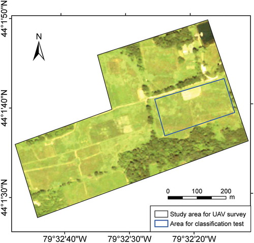
The study area is Koffler Scientific Reserve located in Southern Ontario, Canada (Figure 1). The grasslands in this area mainly consist of species-mixed temperate tall grasses. Dominant grass species in this area are Awnless brome (B. inermis), Goldenrod (Solidago canadensis L.), Milkweed (Asclepias L.), and Fescue (Festuca rubra L.) (Lu and He 2017). Trees and forbs are also widely distributed in this area, interacting with grass growth. Growing season corresponds to the rainy season, starting from May and ending in September or October. Annual total precipitation in this area is from 860 to 1020 mm, with mean temperature from −10°C (February) to 30°C (July) (Environment Canada 2016).

Figure 1. Study area and area selected for classification test. Background is a Quickbird image acquired on 14 July 2013 in true color composition.

UAV missions and field survey

A Tarot T15 Octorotor was used as the UAV platform in this study (Figure 2). It has a weight of 4.5 kg and a frame width of 1.07 m. Ardupilot Mission Planner was applied as the flight control system to control the UAV flight in real time. A minimum of three crew members involved in each flight including a flight manager who is in charge of the flight test, a crew member dedicated to monitoring airspace for other airspace users, and a ground station operator. UAV was monitored by the flight manager as well as all standby pilots throughout the duration of the flights.

Figure 2. UAV system, camera, and a sample photo. Sample photo is NIR–green–blue color composition; vegetation show red color.

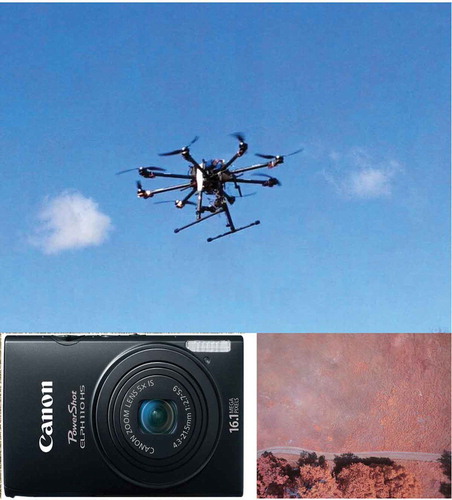
A modified Canon PowerShot ELPH 110HS camera (LDP LLC, Carlstadt, USA) was applied as the imaging sensor in this study (Figure 2). It has NIR, green, and blue channels with central wavelength around 720, 550, and 450 nm, respectively, and produce false color imagery (Figure 2). The manual mode of camera, which specifying shoot parameters such as exposure and ISO, was used to ensure specific incident light conditions. The camera was mounted on a gimbal to leveled out the camera and ensure a vertical (nadir) view (Lu and He 2017).

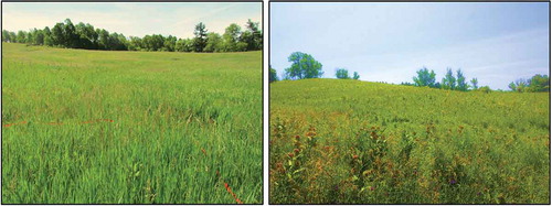
Due to the topographic relief and tree lines in the study area, the UAV was operated at 70 m above the ground that is the lowest safe altitude. Spatial resolution of imagery acquired at this altitude is approximate 5 cm, which is sufficient to identify the dominant species in the study area. The flight speed was about 7 m/s, and images were acquired at 1-s interval that is the highest shooting frequency. The images acquired have an approximately 85% forward overlap and 50% side overlap. Seven flight surveys were conducted from April to December in 2015, aiming to monitor the temporal variation of species composition. Imagery acquired on 11 June and 9 July 2015, which represent a more homogeneous and a more heterogeneous species composition, respectively (Figure 3), was selected in this study.

Figure 3. Photos showing a more homogeneous (left, photo taken on 11 June 2015) and a more heterogeneous (right, photo taken on 9 July 2015) species composition.

Field survey was performed simultaneously with UAV missions. Ground control points (GCPs) (e.g., trees, road intersections) were deployed in the study area, which will be used for the geometric correction of the imagery. Species composition was identified in the field and approximate 80 samples for each dominant species were collected. For Awnless Brome, since it is dense growing in some areas while sparse in some other areas, and these two types have different spectral and textural features, therefore Awnless Brome was separated as two classes: Awnless Brome (dense) and Awnless Brome (sparse). The other classes are Fescue, Goldenrod, and Milkweed. Coordinates of GCPs and sampling sites were recorded using high accuracy Trimble GeoExplorer GPS (Trimble Navigation Limited, Sunnyvale, CA, USA). Other data collected at sampling sites are such as canopy reflectance, vegetation height, and photos.

Imagery processing and classification

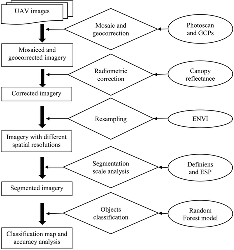
UAV images collected were processed and utilized for species classification following a workflow shown in Figure 4. Details of each procedure will be described in following sections.

Figure 4. Workflow of imagery processing and multi-scale species classification.

Imagery processing

Imagery processing mainly included imagery mosaic, geometric correction, radiometric correction, and pixel resampling to acquire imagery with different spatial resolutions. UAV images were mosaiced using Agisoft PhotoScan 1.2.6 (Agisoft LLC, St. Petersburg, Russia). Geocorrection and orthorectification were also performed in this software using GCPs. The mosaiced and geo-corrected imagery was then radiometrically corrected using an empirical line method with reflectance of ground targets that were collected in the field (Lu and He 2017).

Spatial resolution of corrected imagery is 5 cm. It was resampled in ENVI (Visual Information Solutions Inc., Boulder, Colorado, USA) using the pixel aggregate method to acquire images with spatial resolution of 10, 15, and 20 cm, respectively. Images with spatial resolution of 5, 10, 15, and 20 cm, hereafter, 5-, 10-, 15-, and 20-cm images, were utilized for object-based species classifications.

Species classification

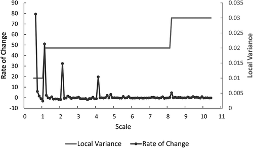
The classification mainly involved two steps: imagery segmentation and object classification. The segmentation was performed using Definiens Developer 7.0 (Definiens AG, Munich, Germany). The segmentation scales were determined using the ESP tool in Definiens (Drǎgu, Tiede, and Levick 2010). Results for imagery acquired on 11 June 2015 with 5-cm spatial resolutions were shown as an example in Figure 5. A few segmentation scales (e.g., 0.6, 1.1, 1.7, 2.1, 4.1, and 8.2) were identified based on LV of objects. After comparing the segmentation results using different scales, it was found that scale 4.1 is able to generate objects that well represent clustery-growing species (e.g., Awnless Brome and Goldenrod), while scale of 0.6 generates objects that well represent solitary-growing species (e.g., Milkweed). Therefore, segmentation was performed at these two scales: (1) segmenting imagery using scale of 4.1 to produce objects with Milkweed (i.e., mixed species) and objects without Milkweed (i.e., pure species), (2) segmenting objects with Milkweed using scale of 0.6 to generate sub-objects that represent pure species (e.g., Milkweed, Fescue). Other parameters were the same for both segmentations, such as 0.1 was used for shape and 0.5 for compactness. For images that have different spatial resolutions, the ESP tool was performed separately to estimate the optimal segmentation scales and images were segmented similarly as described above.

Figure 5. Estimation of scale parameters for multiresolution segmentation of 5 cm image using ESP. The abrupt increases of rate of change (dark grey color curve) indicate the optimal scales for segmentation.

After segmentation, species composition data of field sites were passed onto the corresponding objects. Features of the objects, such as mean reflectance, vegetation indices, and gray level co-occurrence matrix (GLCM) (Lu and He 2017), were calculated in Definiens. The class attributes and object features were imported into RF model (Statistica, StatSoft, Inc., Tulsa, USA) for building classification tree. Half of the samples was applied to train classification models, while the remaining half was utilized for evaluating accuracy of the classification models and producing an error matrix. The error matrixes of classification for images with different spatial resolutions were compared and analyzed to investigate the optimal spatial resolution for classifying different species.

Results and discussion

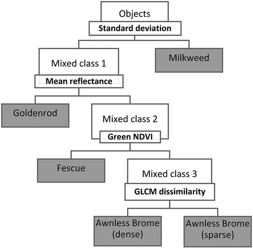
Classification models were built using RF. The model for imagery acquired on 11 June 2015 with 10-cm spatial resolution was shown in Figure 6 as an example. Different features were identified as classifiers for differentiating species at different hierarchies. Specifically, standard deviation was applied to differentiate all objects into Mixed class 1 and Milkweed; mean reflectance was then utilized for classifying Mixed class 1 into Goldenrod and Mixed class 2. Afterwards, green NDVI was calculated for identifying Fescue and Mixed class 3, and lastly, GLCM dissimilarity was used for determining Awnless Brome (dense) and Awnless Brome (sparse) in Mixed class 3.

Figure 6. Classification tree built for imagery acquired on 11 June 2015 with spatial resolution of 10 cm. Classes in the grey colored boxes represent classified species. Bold letters show selected features as classifiers; specific threshold values for different features were not shown for the sake of comprehension.

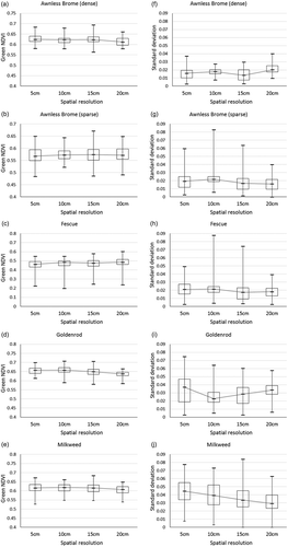
Error matrix of classification model for the image acquired on 11 June 2015 with different spatial resolutions was calculated and shown in Table 1. The overall accuracy for classification of 5-, 10-, 15-, and 20-cm imagery was 82%, 83%, 83%, and 73%, respectively (Table 1). The overall accuracy for classification of 5-, 10-, and 15-imagery is very close. This is expected because we used the same field survey data for the classification, although RF model randomly selected half of data for training and the other half for validating. In addition, the field sites were selected at the center of a small homogeneous area (e.g., pure species), and therefore the decreased spatial resolution from 5 to 15 cm may have a marginal impact on the object features. This can be confirmed in Figure 7, which shows variations of two essential object features, green NDVI and standard deviation, along with decreasing spatial resolution for different species. We can find that the green NDVI and standard deviation changed very slightly when image resolution decreased from 5 to 15 cm. The overall classification accuracy for 20-cm imagery is 73%, much lower than that of the other images. This result indicates that the 20-cm imagery is probably too coarse for species classification in this area.

Table 1. Error matrix of classification model for imagery with different spatial resolutions.

	Predicted
Observed	Awnless brome (dense)	Awnless brome (sparse)	Fescue	Goldenrod	Milkweed	Total	Producer’s accuracy (%)
A
Awnless brome (dense)	28	5	0	0	1	34	82
Awnless brome (sparse)	3	34	1	0	3	41	83
Fescue	0	1	42	0	2	45	93
Goldenrod	4	0	0	37	10	51	73
Milkweed	0	0	0	8	35	43	81
Total	35	40	43	45	51	214	–
User’s accuracy	80%	85%	98%	82%	69%	–	82
B
Awnless brome (dense)	33	3	0	5	0	41	80
Awnless brome (sparse)	4	22	0	0	2	28	79
Fescue	0	5	33	0	0	38	87
Goldenrod	1	0	0	41	2	44	93
Milkweed	5	2	0	4	34	45	76
Total	43	32	33	50	38	196	–
User’s accuracy	77%	69%	100%	82%	89%	–	83
C
Awnless brome (dense)	30	7	0	0	2	39	77
Awnless brome (sparse)	2	26	2	0	3	33	79
Fescue	0	4	28	0	0	32	88
Goldenrod	3	0	0	30	6	39	77
Milkweed	0	2	0	0	42	44	95
Total	35	39	30	30	53	187	–
User’s accuracy	86%	67%	93%	100%	79%	–	83
D
Awnless brome (dense)	22	1	0	0	0	23	96
Awnless brome (sparse)	17	11	5	2	6	41	27
Fescue	0	2	22	1	0	25	88
Goldenrod	3	0	0	22	7	32	69
Milkweed	0	1	0	0	42	43	98
Total	42	15	27	25	55	164	–
User’s accuracy	52%	73%	81%	88%	76%	–	73

Tables A–D correspond to imagery acquired on 11 June 2015 with spatial resolution of 5, 10, 15, and 20 cm, respectively.

Figure 7. Comparison of object features (i.e., green NDVI and Standard deviation) for imagery acquired on 11 June 2015 with different spatial resolutions.

The producer’s and user’s accuracy for the classification of imagery with different spatial resolutions are generally around 80% (Table 1 and Figure 8). Only the producer’s accuracy for Awnless Brome (sparse) and user’s accuracy for Awnless Brome (dense) of 20-cm imagery are much lower, approximately 30% and 50%, respectively (Figure 8). The Awnless Brome, especially the sparse one, is usually mixed with Fescue and Milkweed, which caused considerable misclassification on the 20-cm imagery (Table 1D).

Figure 8. Comparison of producer’s and user’s accuracy of classification using imagery acquired on 11 June 2015 with different spatial resolutions, respectively.

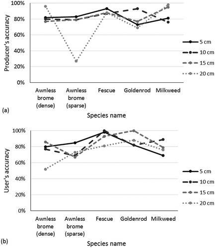
The producer’s accuracy for 5-, 10-, and 15-cm imagery are very close for Awnless Brome (dense) (approximately 80%), Awnless Brome (sparse) (approximately 80%), and Fescue (approximately 90%) (Figure 8a). This is likely because the object features (e.g., green NDVI and standard deviation) of these species only vary slightly on images with different spatial resolutions (Figure 7). However, for Goldenrod and Milkweed, the producer’s accuracy vary greatly among different spatial resolutions. This can be explained by the considerable change of standard deviation on imagery with different spatial resolutions for these two species (Figure 7). In addition, for Goldenrod and Milkweed, the 10- and 15-cm images generate the highest producer’s accuracy. This indicates that it is critical to select imagery with optimal spatial resolution for achieving the best classification results for interested species.

The user’s accuracy for 5-, 10-, and 15-cm imagery is very close for Awnless Brome (dense) (approximately 80%) and Fescue (approximately 90%) (Figure 8b). This indicates that classification of imagery with these three resolutions performs similarly well for identifying the two species. For Awnless Brome (sparse), the 5-cm imagery generated the highest user’s accuracy (85%), indicating that it requires an image with higher spatial resolution to classify this species. As discussed previously, this is mainly because that the Awnless Brome (sparse) is highly mixed with other species. For Goldenrod, the 15-cm imagery produced the highest user’s accuracy (100%). Classification using higher resolution imagery (e.g., 5 or 10 cm) produced lower User’s accuracy (80%). This is probably due to the fact that the Goldenrod is a clustery-growing species with medium density (e.g., more dense than Fescue but less dense than Awnless Brome), resulting in a lot of gaps and shadows within the canopy. The ultrahigh resolution imagery (e.g., 5 or 10 cm) captures these noise features and thus results in a decrease in the classification accuracy. For Milkweed, the 10-cm imagery generated the highest user’s accuracy (90%). Classification using higher (e.g., 5 cm) or lower resolution (e.g., 15 cm) imagery produced lower user’s accuracy (e.g., lower than 80%). This is likely because the 5-cm imagery with detailed features brought noise to the classification; while the 15-cm imagery is too coarse to identify the Milkweed properly. A spatial resolution of 10 cm is coarse enough to omit the noise but fine enough to detect Milkweed species.

Overall, the classification of 10-cm imagery generated good producer’s and user’s accuracy for the species of interest (i.e., Awnless Brome (dense), Goldenrod, and Milkweed). A species composition map was then produced using the imagery acquired on 11 June 2015 with 10-cm spatial resolution (Figure 9a). Similarly, another species composition map for July was generated using the imagery acquired on 9 July 2015 with 10-cm spatial resolution (Figure 9b).

Figure 9. Original images (left, NIR–green–blue color composition) and corresponding classification maps (right). Images were acquired on 11 June and 9 July 2015 and with spatial resolution of 10 cm.

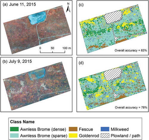
Large spatial and temporal variations of species composition can be noticed in Figure 9. In June (Figure 9c), Awnless Brome was the major dominant species and was densely growing in the central area where is the trough of a slope. Normally, there is higher soil moisture in such areas which contributed to the dense growth of Awnless Brome. In contrast, Fescue was sparsely growing in the crest area of slope (i.e., southern section of the study area) where there is lower soil moisture. Goldenrod was another dominant species and was distributed mainly in the northern section. Milkweed was in the early growing stage and the solitary plants were scattered in the study area. In July (Figure 9d), the species composition was more heterogeneous overall. The distribution area of Awnless Brome (dense) in July is decreased comparing to that in June. Therefore, middle June probably is the peak growing season for Awnless Brome. The distribution of Fescues was not changed clearly and still in the crest area of a slope. Probably, Fescue is the only species that can grow in such relatively drier area. Goldenrod was flourishing in more areas than that in June, which indicates that July is the peak growing season for Goldenrod. Milkweed grew extensively from June to July and was widely distributed in the entire area. Investigating spatiotemporal variations of species composition will contribute to assessing phenological features of different species and further understanding grassland ecosystem, which are essential for the grassland conservation and management.

Summary and future work

Ultrahigh spatial resolution UAV images are a valuable data source for species classification, especially in heterogeneous ecosystems such as grasslands and wetlands. However, using imagery with higher spatial resolution may not necessarily increase the overall accuracy of classification but cost more and pose greater computational challenges. This research demonstrated that the overall accuracy of classification for imagery with 5, 10, and 15 cm is close in our selected grassland, which is expected as the object features varied slightly at these three spatial resolutions. However, for the same species, its producer’s and user’s accuracy are different when using imagery with different spatial resolutions, suggesting that selection of the optimal resolution of imagery is needed for differentiating the targeted species.

Images with different spatial resolutions can be acquired by flying UAV at different altitudes or resampling imagery that has ultrahigh spatial resolution to imagery with coarser resolutions. It is easy to operate UAV at different heights in a small area to collect imagery with different resolutions and identify the optimal resolution(s). However, it is challenging to fly UAV in a large area and at multiple altitudes, which is limited by the battery endurance and time consuming. Resampling an ultrahigh spatial resolution imagery can quickly generate a series of images with different spatial resolutions. One should keep in mind that imagery generated through these two approaches, (1) operating UAV at different altitudes and (2) imagery resampling, may have different spectral or textural information due to the difference in imaging geometry and illumination condition. The resampling process is unavoidable in the process of UAV imagery, such as mosaicing, and geometric and radiometric correction. Future research is warranted to compare imagery obtained from these two approaches.

GEOBIA is an effective tool for species classification using UAV-acquired ultrahigh spatial resolution imagery. Segmentation scales are critical parameters of multiresolution segmentation to obtain imagery objects that represent ground features with different spatial patterns (e.g., clustery- or solitary-growing species). It is critical to determine suitable segmentation scales for imagery with different spatial resolutions. Different tools, such as ESP, can support identifying scales for multiresolution segmentation; however, the users are suggested to test different scales (or scale combinations) and select optimal ones for the ground covers under study. Segmentation strategy in multiresolution segmentation is another factor influencing classification accuracy, for example, which species should be segmented first, and multi-level segmentation should be top-down or bottom-up. One is encouraged to test different segmentation strategies and identify the best approach.

RF modeling is powerful as it builds the classification tree quickly and accurately. Training samples and object features that are imported into RF model are critical factors influencing performance of RF. Since there may be substantial variations of object spectral and textural features within one species resulting from the ultrahigh spatial resolution of imagery, the selected samples should cover as much as these variations and researchers are suggested to analyze the object spectral and textural features before importing them into RF model. This will help to further understand the features identified by RF as classifiers. In addition, there are a great number of object features available in GEOBIA, such as spectral, textural, or geometrical based. Importing different features into RF model will possibly generate different classification models with different accuracies. Furfure research evaluating characteristics of object features is encouraged before importing them into RF, and the focuses could be placed on which features are more important for what types of classification.

Species composition in the study area shows clear temporal variations. Investigating spatiotemporal variations of species composition is essential for monitoring vegetation community structure, identifying ecologically and economically important species, and understanding ecosystem health. The results are expected to support the ecosystem conservation and management. UAV has high flexibility to collect multi-temporal imagery for phenological analysis. However, UAV images acquired at different times need to be calibrated (e.g., radiometric calibration) for a quantitative comparison, such as comparing object features (e.g., NDVI). Object features calculated using raw imagery (e.g., in digital numbers) are not temporally comparable since the digital numbers are influenced by the illumination condition.

Acknowledgments

This work was supported by the Natural Sciences and Engineering Research Council of Canada (NSERC): [Discovery Grant Number RGPIN-386183] to Dr. Yuhong He; and the Department of Geography, University of Toronto Mississauga under Graduate Expansion Funds. We thank the UAV flight crew from Arrowonics Technology Ltd. for the imagery collection and the managers of the Koffler Scientific Reserve for help setting up field sites. Assistance from lab technician Phil Rudz and a group of students at the University of Toronto Mississauga is acknowledged. Also thanks to Transport Canada for providing a Special Flight Operating Certificate: [Number 5812-15-14-2016-1 and 5812-15-14-2014-3].

Disclosure statement

No potential conflict of interest was reported by the authors.

Additional information

Funding

This work was supported by the Natural Sciences and Engineering Research Council of Canada: [Discovery Grant Number RGPIN-386183]; Department of Geography, University of Toronto Mississauga: [Graduate Expansion Funds]

References

- Anderson, T. M., K. L. Metzger, and S. J. McNaughton. 2007. “Multi-Scale Analysis of Plant Species Richness in Serengeti Grasslands.” Journal of Biogeography 34 (2): 313–323. doi:10.1111/j.1365-2699.2006.01598.x.
- Belgiu, M., and L. Drăguţ. 2016. “Random Forest in Remote Sensing: A Review of Applications and Future Directions.” ISPRS Journal of Photogrammetry and Remote Sensing 114: 24–31. doi:10.1016/j.isprsjprs.2016.01.011.
- Bertalan, L., Z. Túri, and G. Szabó. 2016. “UAS Photogrammetry and Object-Based Image Analysis (Geobia): Erosion Monitoring at the Kazár Badland, Hungary.” Landscape & Environment 10 (3–4): 169–178. doi:10.21120/LE/10/3-4/10.
- Chen, G., M. R. Metz, D. M. Rizzo, W. W. Dillon, and R. K. Meentemeyer. 2015. “Object-Based Assessment of Burn Severity in Diseased Forests Using High-Spatial and High-Spectral Resolution Master Airborne Imagery.” ISPRS Journal of Photogrammetry and Remote Sensing 102: 38–47. doi:10.1016/j.isprsjprs.2015.01.004.
- Chen, G., K. Zhao, and R. Powers. 2014. “Assessment of the Image Misregistration Effects on Object-Based Change Detection.” ISPRS Journal of Photogrammetry and Remote Sensing 87: 19–27. doi:10.1016/j.isprsjprs.2013.10.007.
- Dalponte, M., H. O. Orka, T. Gobakken, D. Gianelle, and E. Naesset. 2013. “Tree Species Classification in Boreal Forests with Hyperspectral Data.” IEEE Transactions on Geoscience and Remote Sensing 51 (5): 2632–2645. doi:10.1109/TGRS.2012.2216272.
- Drǎgu, L., D. Tiede, and S. R. Levick. 2010. “Esp: A Tool to Estimate Scale Parameter for Multiresolution Image Segmentation of Remotely Sensed Data.” International Journal of Geographical Information Science 24 (6): 859–871. doi:10.1080/13658810903174803.
- Environment Canada. 2016. “Historical Climate Data.” Accessed 20 July 2016. http://climate.weather.gc.ca/
- Hall, K., L. J. Johansson, M. T. Sykes, T. Reitalu, K. Larsson, and H. C. Prentice. 2010. “Inventorying Management Status and Plant Species Richness in Semi-Natural Grasslands Using High Spatial Resolution Imagery.” Applied Vegetation Science 13 (2): 221–233. doi:10.1111/avsc.2010.13.issue-2.
- Hardin, P. J., and R. R. Jensen. 2011a. “Small-Scale Unmanned Aerial Vehicles in Environmental Remote Sensing: Challenges and Opportunities.” GIScience & Remote Sensing 48 (1): 99–111. doi:10.2747/1548-1603.48.1.99.
- Hardin, P. J., and R. R. Jensen. 2011b. “Introduction-Small-Scale Unmanned Aerial Systems for Environmental Remote Sensing.” GIScience & Remote Sensing 48 (1): 1–3. doi:10.2747/1548-1603.48.1.1.
- Hay, G. J., and G. Castilla. 2008. Geographic Object-Based Image Analysis (Geobia): A New Name for a New Discipline. Berlin, Heidelberg: Springer Berlin Heidelberg.
- Hooper, D. U., and P. M. Vitousek. 1997. “The Effects of Plant Composition and Diversity on Ecosystem Processes.” Science 277 (5330): 1302–1305. doi:10.1126/science.277.5330.1302.
- Huang, C., E. L. Geiger, W. J. D. Van Leeuwen, and S. E. Marsh. 2009. “Discrimination of Invaded and Native Species Sites in a Semi‐Desert Grassland Using MODIS Multi‐Temporal Data.” International Journal of Remote Sensing 30 (4): 897–917. doi:10.1080/01431160802395243.
- Jensen, J. R. 2006. Remote Sensing of the Environment: An Earth Resource Perspective. Upper Saddle River: Prentice Hall.
- Knoth, C., B. Klein, T. Prinz, and T. Kleinebecker. 2013. “Unmanned Aerial Vehicles as Innovative Remote Sensing Platforms for High-Resolution Infrared Imagery to Support Restoration Monitoring in Cut-Over Bogs.” Applied Vegetation Science 16 (3): 509–517. doi:10.1111/avsc.12024.
- Laliberte, A. S., and A. Rango. 2009. “Texture and Scale in Object-Based Analysis of Subdecimeter Resolution Unmanned Aerial Vehicle (UAV) Imagery.” IEEE Transactions on Geoscience and Remote Sensing 47 (3): 761–770. doi:10.1109/TGRS.2008.2009355.
- Laliberte, A. S., and A. Rango. 2011. “Image Processing and Classification Procedures for Analysis of Sub-Decimeter Imagery Acquired with an Unmanned Aircraft over Arid Rangelands.”.” GIScience & Remote Sensing 48 (1): 4–23. doi:10.2747/1548-1603.48.1.4.
- Langley, S. K., H. M. Cheshire, and K. S. Humes. 2001. “A Comparison of Single Date and Multitemporal Satellite Image Classifications in a Semi-Arid Grassland.” Journal of Arid Environments 49 (2): 401–411. doi:10.1006/jare.2000.0771.
- Lu, B., and Y. He. 2017. “Species Classification Using Unmanned Aerial Vehicle (UAV)-Acquired High Spatial Resolution Imagery in a Heterogeneous Grassland.” ISPRS Journal of Photogrammetry and Remote Sensing 128:73-85. doi:10.1016/j.isprsjprs.2017.03.011.
- Lu, B., Y. He, and H. Liu. 2016. “Investigating Species Composition in a Temperate Grassland Using Unmanned Aerial Vehicle-Acquired Imagery.” 2016 4th International Workshop on Earth Observation and Remote Sensing Applications (EORSA, 107–111. doi:10.1109/EORSA.2016.7552776.
- Ma, L., L. Cheng, M. Li, Y. Liu, and X. Ma. 2015. “Training Set Size, Scale, and Features in Geographic Object-Based Image Analysis of Very High Resolution Unmanned Aerial Vehicle Imagery.” ISPRS Journal of Photogrammetry and Remote Sensing 102: 14–27. doi:10.1016/j.isprsjprs.2014.12.026.
- Manuel Pena, J., J. Torres-Sanchez, A. Isabel De Castro, M. Kelly, and F. Lopez-Granados. 2013. “Weed Mapping in Early-Season Maize Fields Using Object-Based Analysis of Unmanned Aerial Vehicle (UAV) Images.” Plos One 8 (e7715110). doi:10.1371/journal.pone.0077151.
- Martin, M. E., S. D. Newman, J. D. Aber, and R. G. Congalton. 1998. “Determining Forest Species Composition Using High Spectral Resolution Remote Sensing Data.” Remote Sensing of Environment 65 (3): 249–254. doi:10.1016/S0034-4257(98)00035-2.
- Nebiker, S., A. Annen, M. Scherrer, and D. Oesch. 2008. “A Light-Weight Multispectral Sensor for Micro UAV—Opportunities for Very High Resolution Airborne Remote Sensing.” International Archives of the Photogrammetry, Remote Sensing and Spatial Information Sciences 37: 1193–1200.
- Puissant, A., S. Rougier, and A. Stumpf. 2014. “Object-Oriented Mapping of Urban Trees Using Random Forest Classifiers.” International Journal of Applied Earth Observation and Geoinformation 26: 235–245. doi:10.1016/j.jag.2013.07.002.
- Rodriguez-Galiano, V. F., B. Ghimire, J. Rogan, M. Chica-Olmo, and J. P. Rigol-Sanchez. 2012. “An Assessment of the Effectiveness of a Random Forest Classifier for Land-Cover Classification.” ISPRS Journal of Photogrammetry and Remote Sensing 67: 93–104. doi:10.1016/j.isprsjprs.2011.11.002.
- Stumpf, A., and N. Kerle. 2011. “Object-Oriented Mapping of Landslides Using Random Forests.” Remote Sensing of Environment 115 (10): 2564–2577. doi:10.1016/j.rse.2011.05.013.