Regional-scale monitoring of cropland intensity and productivity with multi-source satellite image time series

Abstract

In the context of growing populations and limited resources, the sustainable intensification of agricultural production is of great importance to achieve food security. As the need to support management at a range of spatial scales grows, decision-support tools appear increasingly important to enable the timely and regular assessment of agricultural production over large areas and identify priorities for improving crop production in low-productivity regions. Understanding productivity patterns requires the timely provision of gapless, spatial information about agricultural productivity. In this study, dense 30-m time series covering the 2004–2014 period were generated from Landsat and MODerate-resolution Imaging Spectroradiometer (MODIS) satellite images over the irrigated cropped area of the Fergana Valley, Central Asia. A light-use efficiency model was combined with machine learning classifiers to assess the crop yield at the field level. The classification accuracy of land cover maps reached 91% on average. Crop yield and acreage estimates were in good agreement (R² = 0.812 and 0.871, respectively) with reported yields and acreages at the district level. Several indicators of cropland intensity and productivity were derived on a per-field basis and used to highlight homogeneous regions in terms of productivity by means of clustering. Results underlined that regions with lower water-use efficiency were not only located further away from irrigation canals and intake points, but also had limited access to markets and roads. The results underline that yield could be increased by roughly 1.0 and 1.4 t/ha for cotton and wheat, respectively, if the access to water would be optimized in some of the regions. The minimum calibration requirement of the method and the fusion of multi-sensor data are keys to cope with the constraints of operational crop monitoring and guarantee a sustained and timely delivery of the agricultural indicators to the user community. The results of this study can form the baseline to support regional land- and water-resource management.

Keywords:

• agricultural management
• cropland use intensity
• crop yield
• crop type classification
• water-use efficiency

Introduction

The most intensive cropping systems, with several harvests per year, occur in dry areas where irrigation is widespread (Salmon et al. 2015; Xiao et al. 2006). Irrigated agriculture covers 16–20% of the total arable area, but contributes to circa 44% of total crop production (Alexandratos and Bruinsma 2012). However, it is also the world´s largest source of freshwater consumption (Bastiaanssen, Molden, and Makin 2000; Sauer et al. 2010). With the soaring demography and the limited potential to expand the suitable cropped areas as backdrop, irrigation is expected to become an increasingly important practice to meet the global food demand (Wichelns and Oster 2006). Irrigation may lead to waterlogging, increased salinization (Abbas et al. 2010; Singh 2015), and land degradation (Dregne 2002; Gibbs and Salmon 2015; United Nations 2015) which in turn affect the productivity as they lower yields below their potential (Aslan and Gundoglu 2007; Bahçeci et al. 2006; Lobell et al. 2009; Singh 2010). Since many irrigation systems perform below their potential, it becomes critical to evaluate their actual productivity to assess potential yield gaps (Lobell et al. 2005).

One prominent example of irrigated agriculture in dry areas is the Fergana Valley in Central Asia where agriculture suffers from low field application efficiencies (Pereira et al., 2009; Reddy et al., 2013), and where percolation and transpiration losses render agricultural productivity ineffective (Horst et al., 2005; Reddy et al., 2013). For instance, the yields of cotton, the main crop since the 1960s (Abdullaev et al., 2009a), decreased from 4.6 t/ha in 1980 to 2.9 t/ha in 2000 (SIC-ICWC, 2016) due to widespread land degradation and soil salinization (Ibrakhimov et al. 2007). Other factors such as climate change or agricultural management practices could further lead to a significant drop in production (Abdullaev et al. 2009b; Bichsel 2009). Therefore, understanding the dynamics of water-use efficiency, crop productivity, and their constraints in both space and time would support the identification of options for increasing productivity and cropping intensity in a sustainable fashion. This is particularly notable in view of recent changes in Uzbekistan’s strategy to significantly cut cotton output by 2020 and devote unproductive lands to alternative crops such as vegetable, potato, and forage production.

The integrated use of geographical information systems (GIS), satellite imagery, crop models, and machine-learning algorithms is an efficient means for tracking the dynamics of agricultural productivity in space and time as well as providing decision-support tools (Roberts et al. 2009; Tayyebi et al. 2016a; Tayyebi et al. 2016b; Johnson 2014; Kussul et al. 2012; Matton et al. 2015). An array of indicators of agricultural productivity has been devised to assess (a) cropland dynamics (De Beurs and Ioffe 2014; Li et al. 2014), (b) cropping intensity (Estel et al. 2016; Kuemmerle et al. 2013; Löw, Conrad, and Michel 2015a; Löw et al. 2015b; Martinez-Casasnovas, Martín-Montero, and Auxiliadora Casterad 2005; Peña-Barragán et al. 2011; Shao et al. 2009), (c) biophysical variables such as biomass or leaf area index which are required for yield estimation (Alganci et al. 2014; Doraiswamy et al. 2005; Duveiller, Baret, and Defourny 2011; Haboudane et al. 2002; Li et al. 2015; Lobell 2013), (d) irrigation and water-use efficiency (Bastiaanssen, Molden, and Makin 2000; Bastiaanssen and Bos 1999; Liu et al. 2010; Sepulcre-Cantó et al., 2013), (e) soil salinity (Metternicht and Zinck 2003), and (f) land degradation (Abbas et al. 2010; Dubovyk et al. 2013; Skakun et al. 2015). In addition, remote sensing can support crop insurance through assessment (De Leeuw et al. 2014) or mitigation of crop pest infestations (Latchininsky 2013; Löw et al. 2016b; Renier et al. 2015; Waldner et al. 2015).

From a management point of view, satellite remote sensing has several advantages for operational and reliable crop monitoring. First, it has the ability to bypass or complement in situ measurements, which is specifically important in regions such as the Fergana Valley where access to such information is limited. Second, it can provide estimates at a range of spatial scales, which in turn may reduce the reliance on aggregated statistics. Third, it enables both nowcasting and hindcasting using archive imagery, enabling the understanding inter-annual variations in productivity (Lobell et al. 2005). However, one drawback of using certain satellite systems is that they provide images either too coarse for field-level assessments, e.g., MODerate-resolution Imaging Spectroradiometer (MODIS; Duveiller 2011; Löw and Duveiller 2014), or with insufficient temporal frequency that hampers continuous modelling, e.g., Landsat (Lobell et al. 2015).

Bearing these limitations in mind, this article evaluates a set of methods for crop productivity assessment at the field level and its ability to simultaneously respond to users’ needs and cope with operational constraints. Based on user consultations with regional (Scientific-Information Center of the Interstate Commission for Water Coordination in Central Asia, SIC-ICWC) and international organizations (International Center for Agricultural Research in the Dry Areas, ICARDA), the methods seek to provide end-of-season crop production estimates as well as increase the diagnostic capability and the understanding of the cropland-use intensity in the Fergana Valley. Therefore, descriptors of land-use intensity, crop yield, and water-use efficiency were thus produced on annual and multi-annual bases and used to highlight spatial and temporal patterns of productivity. Because operational monitoring cannot tolerate compromises in the integrity of the product due to the inability to collect remote sensing and in situ data or technical hazards such as sensor failure, data collection cancellation, or high cloud coverage, special care was devoted to: (a) ensure that sufficient satellite data would be available through the use of multi-sensor imagery fusion and (b) integrate methods with minimum calibration data requirements and high generalization capabilities.

Study site and data

Study site

The Fergana Valley is located in the Aral Sea Basin, a vast transboundary river basin at the heart of the Eurasian continent, and surrounded by the Alatau Range in the North, the Tian Shan Mountains in the East, and the Alay Mountains in the South (Figure 1). The valley spans in the upstream region of Central Asia’s most important irrigated region (Abdullaev et al. 2009b; Bichsel 2009). This region became most known for the desiccation of the Aral Sea (Löw et al. 2013b; Micklin 2016), caused by the expansion of irrigation agriculture along the Amu Darya and Syr Darya rivers during the Soviet period (Saiko and Zonn 2000). The Fergana Valley is located around the upper and mid-reach of the Syr Darya river catchment that generates almost 70% of surface water (SIC-ICWC 2016). It virtually represents the sole source of water for irrigation. Climate is continental dry with 100–200 mm average annual precipitation in the flat valley floor (Munoz and Grieser 2006).

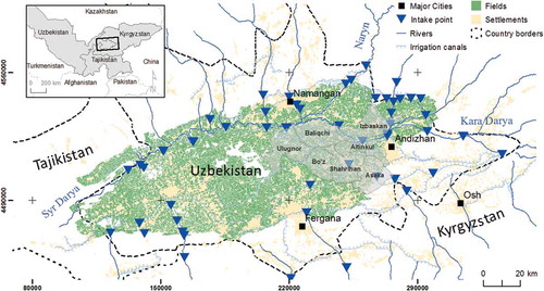
Figure 1. Cropland distribution in the Fergana Valley. Rivers, intake points, and irrigation canals are shown in shades of blue. The settlements, in yellow, were derived by means of on-screen digitization of GoogleEarth™ images from 2016. Crop yield and acreage statistics were available for the districts in the eastern and south eastern parts solely (grey polygons).

Cotton is the dominant crop in the region (Abdullaev et al. 2009b), though it has been progressively supplemented by winter wheat after the independence from the Union of Soviet Socialist Republics in 1991 (Abdullaev et al. 2009b). Cotton is sown mid-April and harvested from September to October. Winter wheat is generally sown in autumn, and its harvest spans from June to July, depending on the actual sowing date. After winter wheat, a second crop such as sorghum or maize is usually cultivated. In addition, various vegetables, e.g., carrots or beans, melons, and fruit trees are grown.

Satellite data

Satellite image time series from MODIS and Landsat covering a 11-year period from 2004 to 2014 were at hand. On the one hand, 8-Day MODIS surface reflectance data (250 m) were downloaded (MOD09Q1; tile h23v04). In total, 46 images were available for each year and stacked into 11 annual time series. On the other hand, 319 Landsat TM, ETM+, and OLI images (30 m) were available (two tiles: path 152/row 032 and path 153/row 032). The average Landsat data availability was 12 images per year with a minimum of seven (2007) and maxima of 20 (2008).

Field boundaries and in situ data

Field boundaries were digitized based on GoogleEarth™ satellite images from 2016. The resulting database totalled 87,883 field entries, which covered an area of 6,362.15 km². The average field size is 6.74 ha which was found sufficiently large to identify crop classes using 30-m data (Löw and Duveiller 2014). Fields above 500 m of elevation were not digitized because: (a) they were generally too small to be resolved at Landsat’s resolution and (b) the number of usable images dropped markedly due to the more persistent cloud cover.

In 2014, in-situ data of the major crop types were randomly collected throughout the study region (Table 1). In addition, reference samples for 2010–2012 were extracted from existing field-based land cover maps (Conrad et al. 2013b; http://geonode.caiag.kg, last access 09/09/2015) and cross-checked by visual inspection of Normalized Difference Vegetation Index (NDVI) signatures. In total, seven classes were of interest: “Cotton,” “Winter wheat-Other,” “Orchards,” “Fallow,” “Rice,” “Other crops,” and “Fishponds.” The class “Winter wheat-Other” is an intra-annual sequence of winter wheat followed by a summer crop (usually rice, sorghum, or maize). Orchards include perennial woody vegetation such as fruit tree plantations or vineyards. “Fallow” fields were neither tilled nor sowed in the survey year. “Other” groups the remaining marginal crops for which insufficient reference data was available.

Table 1. Number of reference fields per year and per crop. In total, there were 3,211 fieldswith known crop type.

Class	Number of reference fields
	2010	2011	2012	2014
Cotton	240	160	262	234
Winter wheat – Other	244	266	190	200
Orchards	124	114	137	102
Fallow	77	116	115	55
Rice	67	95	61	50
Other crops	130	20	56	30
Fishponds	15	18	19	14
Total number	897	789	840	685

Crop area, yield, and ancillary data

Agricultural statistics from seven districts of the Fergana Valley including in-situ crop yield (in tons per hectare for wheat and cotton) and crop acreage, aggregated at the district level, were available (SIC-ICWC 2016) for the years 2010–2012. Several ancillary datasets were also at hand, namely: the locations of irrigation canals and roads were sourced from OpenStreetMap, the location of intake points was sourced from SIC-ICWC (2016), and the location of the settlements was obtained via Google Earth^TM imagery.

The Global Agro-Ecological Zones (GAEZ) dataset, version 3.0., which is based on the Harmonized World Soil Database (HWSD) and climate data for 1961–1990 (Fischer et al. 2002; IIASA and FAO, 2012), was taken from the Food and Agriculture Organization (FAO). It provides a description of the environmental characteristics of a region as well as the crop-suitability index for several crop types.

Methods

The assessment of crop productivity consists in five consecutive steps (Figure 2). First, Landsat and MODIS images were pre-processed and fused to produce 8-day synthetic time series at 30 m (Section 3.1). Second, crop types were identified at the field level based on NDVI signatures (Section 3.2) The third step focused on yield estimation (Section 3.3), which is the prerequisite for assessing the water-use efficiency (Section 3.4). The fifth module sought to derive several indicators of agricultural intensity and productivity (Section 3.5). Finally, these indicators were utilized to identify and map homogeneous regions of similar productivity profile by means of clustering.

Figure 2. Workflow of the method and its associated maps: crop type, crop yield, water-use efficiency, agricultural indicators, and identification of homogeneous areas.

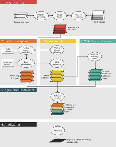
Image data pre-processing

Multi-temporal classification often relies on vegetation indices like NDVI (Rouse et al. 1974) to capture phenological changes of different vegetation classes. Therefore, a time series of Landsat-like NDVI images was generated by blending NDVI images from Landsat and MODIS using the ESTARFM method (Gao et al. 2006; Zhu et al. 2010). An “index-then-blend” approach was implemented as it was reported to be more accurate and less computationally expensive than blending reflectance values before calculating NDVI (Jarihani et al. 2014; Knauer et al. 2016).

Two pre-processing steps were applied to reduce effects of clouds and aerosols and construct consistent time series. First, Landsat-7 ETM+ data acquired after the scan line corrector failure (31 May 2003) were gap-filled using on the algorithm developed by Chen et al. (2011) and clouds were masked based on the results of Fmask (Zhu and Woodcock 2012). Second, MODIS pixels labelled as no-data, snow/ice, or clouds were excluded based on the quality flags. To minimize the impact of outliers and restore missing values, the MODIS time series were smoothed using the approach developed by Chen et al. (2004).

The ESTARFM fusion operates at the pixel level and requires pairs of Landsat and MODIS images. Linear regressions were fitted for a central pixel within a moving window. Within the moving window, all pixels that are spectrally similar to the central pixel are considered. At least one Landsat-MODIS image pair for approximately the same day was required, followed by a MODIS image corresponding to the next day for which the fused Landsat images can be generated (Figure 3). MODIS images were re-projected to the same projection as the Landsat data (Asia North Albers Equal Area Conic, ESRI: 102,025) and resampled to 30 m using the nearest-neighbour algorithm. The available Landsat/MODIS base pairs were then fused individually with a 1,500 m by 1,500 m window size (Gao et al. 2006). The accuracy of the synthetic images was evaluated by comparing the predicted NDVI with the corresponding Landsat NDVI of 2,500 random samples and for each image pair annually. The prediction accuracy was quantified in terms of median Pearson´s correlation coefficient (R²) and median Root Mean Square Error (RMSE) across observation years.

Figure 3. Example of data fusion of NDVI could free maps in 2004. Left: original Landsat-7 image with SLC-off, middle: MODIS image, right: cloud- and gap-free synthetic image.

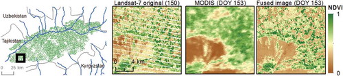
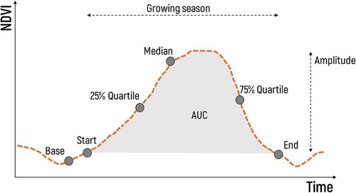
Figure 4. Generalized scheme of NDVI phenological metrics for the growing season. The phenological metrics are in fact statistical descriptors of the NDVI trajectory of a field.

Crop type classification and validation

Capitalizing on the field boundary dataset, a per-field classification method was implemented. For every year and every image, field-level average and standard deviation NDVI values were computed and served as predictor variables. To improve class discrimination, eight phenology metrics were additionally derived (Figure 4):

• The median NDVI value of the total growing season;

• The 25% and 75% percentile of NDVI value of the total growing season;

• Amplitude of the total growing season;

• Start and end of growing season;

• Length of the total growing season; and

• The area under the curve (AUC) between the start to the end of the growing season.

Such metrics were found to enhance the classification accuracy when used instead or in addition to raw time series data (Alcantara et al. 2012; Jacquin, Sheeren, and Lacombe 2010). The growing season was determined based on results from TIMESAT (Jonsson and Eklundh 2004).

Random Forests (RF; Breiman 2001) and Support Vector Machines (SVM; Cortes and Vapnik 1995) were calibrated as base classifiers and configured according to the decision-fusion approach developed by Löw, Conrad, and Michel (2015a). This method consists in randomly selecting subsets from the full set of predictor variables, calibrate a RF and SVM classifier for each subset, and then fuse the results according to a weighted majority-voting scheme. Weights were defined in proportion to the corresponding classification uncertainty at the pixel level (Policar 2006). In this study, each subset contained half of the predictor variables and 50 random draws were performed. To identify crop types in years without ground truth data, the reference data-sets were pooled together to calibrate one unified classifier algorithm (Hüttich et al. 2011; Löw et al. 2016b; Zhong, Gong, and Biging 2014).

The accuracy of the annual crop maps was assessed based on independent validation samples. Confusion matrices were calculated to estimate overall (Congalton 1991) and class-wise (F-score) accuracies (Van Rijsbergen 1979). In addition, receiver operating characteristic curves (ROC) and the corresponding area under the ROC curves (AUC), which is an increasingly used accuracy metric in machine learning and data mining (Fawcett 2006; Tayyebi et al. 2014; Tayyebi and Pijanowski 2014), have been calculated. By averaging the AUC over the different classes, an overall measure for the quality of the model predictions is obtained (Loosvelt, Peters, and Skriver 2012a):

$AU{C}_{avg}=\sum _{i=1}^{c}AUC\left(i\right)\ast w\left(i\right)$

with $c$ the number of classes (here c = 7), $AUC\left(i\right)$ the area under the ROC curve for land cover class $i$, and $w\left(i\right)$ the weighing factor associated with class $i$. This weighing factor is determined with respect to the contribution of each class in the test dataset.

Crop yield estimation and validation

Methods to derive crop yields range from empirical relationships between satellite-derived vegetation indices and ground-based yield measurements over official statistics (Bolton and Friedl 2013) to more sophisticated crop simulation models but with high input data requirements (Doraiswamy et al. 2004; Doraiswamy et al. 2005). Models based on light use efficiency (LUE; Monteith and Moss 1977) were shown to provide accurate yield estimates (Alganci et al. 2014; Lobell 2013; Lobell et al. 2003) and do not heavily depend on in-situ calibration data (Lobell 2013; Sadras et al. 2015). The LUE model is based on the assumption that biomass production is proportional to total absorption of Photosynthetically Active Radiation (PAR) over the course of the growing season (Vanino et al. 2015). It has several main terms: (a) the fraction of PAR absorbed by the vegetation canopy (fPAR), (b) the LUE term that describes the light-to-biomass conversion efficacy of the investigated crop, and (c) coefficients needed to convert biomass to harvestable yield, including harvest index ($\mathrm{H}\mathrm{I}$). Mathematically, it reads as:

(1) $Y_{crop}=\left(\sum _{SoS}^{EoS}fPAR\ast PAR\ast LU{E}_{act}\right)\ast HI$(1)

where ${\mathrm{Y}}_{\mathrm{c}\mathrm{r}\mathrm{o}\mathrm{p}}$ is final crop yield (in g × m⁻²), SoS and EoS are the start and end of season, $\mathrm{L}\mathrm{U}{\mathrm{E}}_{\mathrm{a}\mathrm{c}\mathrm{t}}$ is the actual light use efficiency (in gC × MJ⁻¹),PAR is the photosynthetic active radiation (in W × m⁻²). In fact, the product in the brackets represents the daily accumulation of aboveground biomass integrated over the growing season. The fraction of photosynthetic active radiation (fPAR) for each field was derived from the synthetic NDVI values using generic NDVI-fPAR equations (Sellers et al. 1996) – an approach that already gave reasonable results and could be applied independently from fPAR field measurements (Alganci et al. 2014; Lex et al. 2015; Lobell, Ortiz-Monasterio, and Lee 2010; Lobell et al. 2003).

Due to the arid climate, the LUE had to incorporate plant stresses by applying certain stress factors, which limit biomass accumulation and thus crop yields:

(2) $LU{E}_{act}=\epsilon \ast T^{\prime }\ast W^{\prime }$(2)

where $\mathrm{L}\mathrm{U}{\mathrm{E}}_{\mathrm{a}\mathrm{c}\mathrm{t}}$ represents the daily actual light-use efficiency, $\epsilon$ is the maximum crop-specific LUE (cotton: 1.9, wheat: 2.0), ${\mathrm{T}}^{\prime }$ represents temperature and ${\mathrm{W}}^{\prime }$ water-induced stresses (both scaled between 0 and 1). The crop stress scalars were calculated from meteorological measurements and the ratio between actual evapotranspiration (ET_act) and crop evapotranspiration (ET_c). ET_act was assessed for each field using the S-SEBI (Simplified Surface Energy Balance Index) algorithm (Löw et al. 2016a; Roerink, Su, and Menenti 2000; Senay et al. 2013) and ET_c was calculated according to Allen et al. (1998). Crop yield is finally derived by applying $HI$ (cotton: 0.25, wheat 0.38) at the end of the season recalculation to t × ha⁻¹. Values for $HI$ and $\epsilon$ were provided by SIC-ICWC (2016), based on field measurements, and were within the range of other studies (Hunink and Droogers 2011; Lobell, Ortiz-Monasterio, and Lee 2010; Steduto et al. 2009; Fritsch 2013; Shi et al. 2007).

The coefficient of determination (R²), and the root mean square error (RMSE) were used for assessing the estimates of crop yields and crop acreage based on district-level statistics.

Water-use efficiency

Crop-specific water-use efficiencies were produced by dividing crop yield with the estimated seasonal water use, based on ET_act (Section 3.3), and using a straightforward approach that relies only on remotely sensed data (Biradar et al. 2008; Platonov et al. 2008; Sadras et al. 2015):

(3) $WU{E}_{crop}=\frac{Y_{crop}}{E{T}_{act}}$(3)

where $WU{E}_{crop}$is the water-use efficiency in kg/m³.

Indicators of agricultural productivity

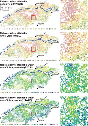
Four indicators of cropping intensity and two indicators of productivity were computed from the annual crop type, yield, and WUE maps, namely: (a) cropping frequency, (b) fallow cycles, (c) number of annual multi-cropping, (d) major crop class, (e) ratio actual versus attainable crop yield, and (f) ratio actual versus attainable WUE (see Table 2).

Table 2. Multi-year cropland use intensity indicators, their purpose, and selected references.

Description	Formula	Purpose of use and options for management	References
Cropping frequency (CF)
Cropland-use intensity, counts the number of years $i$ a field was used/harvested. In this study, the maximum number of years $Y$ was 11 (2004–2014)	$\mathrm{C}\mathrm{F}=\sum _{\mathrm{i}=1}^{\mathrm{Y}}\mathrm{y}\left(\mathrm{i}\right)$	Facilitates identification of land affected by land degradation, and priority sites for alternative land use options. Supports assessment of potentials for intensification and the identification of abandoned land.	Alcantara et al. (2012); Dubovyk et al. (2013); Estel et al. (2016); Löw et al. (2016c)
Fallow cycles (FCI)
Number of recurring, consecutive sequences of fallow cropland (i.e., not sown, cropped, or ploughed). Recurring periods of 1 (S1), 2 (S2), and 3 years (S3) were considered. $N_S$ gives the maximum number of possible sequences in the observation period (e.g. 6 times S1). The maximum number of years $Y$ was 11 (2004–2014).	$FCI=\sum _{i=1}^{N_{S1}}\left(S1\ast \frac{N_{S1}}{Y}\right)+\left(S2\ast \frac{N_{S2}}{Y}\right)+\left(S3\ast \frac{N_{S3}}{Y}\right)$	Supports assessing management practices (fallow periods, soil regeneration) and intensity of land management.	Estel et al. (2016)
Multi cropping (MC)
Number of harvests over several years. The class wheat-other equals to 2 harvests, the class fallow equal to zero harvest, the reminder classes equal to one harvest.	$\mathrm{M}\mathrm{C}=0.5\ast \sum _{\mathrm{i}=2}^{22}\mathrm{s}\left(\mathrm{i}\right)$	Assessment of cropping intensity, crop practices and input demands (irrigation water, fertilizer)	Christmann et al. (2009); Estel et al. (2016)
Major crop class (MOD)
Most frequently (modus) cultivated crop in the observation period.	$\mathrm{M}\mathrm{O}\mathrm{D}=\bar{x}\left(i\right)$	Enables identification of monoculture, assessment of environmental impact of monoculture (e.g. land degradation, reduction of soil fertility), track diversification of cropping systems toward more integrative systems, for example double cropping with wheat or intercropping (not assessed in this study), interventions to sustain food production	Christmann et al. (2009)
Ratio actual vs. attainable crop yield (RYIELD)
Ratio of actual yield (as median crop yield over years) to attainable yield defined as the 95% percentile $Y_{95}$on the probability density function of crop yield.	$RYIELD=\frac{\overline{Y_{crop}}}{Y_{95}}$	Facilitates identification of local yield gaps and yield growth opportunities. Enables assessment of yield constraining factors.	Lobell (2013); Lobell, Ortiz-Monasterio, and Lee (2010); Sadras et al. (2015)
Ratio actual vs. attainable WUE (RWUE)
Ratio of actual WUE (as median WUE yield over years) to attainable WUE defined as the 95% percentile $WU{E}_{95}$on the probability density function of WUE.	$RWUE=\frac{\overline{WU{E}_{crop}}}{WU{E}_{95}}$	Facilitates identification of opportunities for improving WUE. Supports assessing potentials to save irrigation water, and manageable and agro-ecological system properties that determine spatial pattern of WUE.	Bastiaanssen and Harshadeep (2005); Cai et al. (2011); González-Dugo and Mateos (2008); Molden and Sakthivadivel (1999)

First, the cropping frequency (CF) is defined as the number of years $y$ out of all observed years $Y$ when a field was cropped, i.e., not classified as “fallow.” Next, consecutive sequences of fallow cycles (FCI) defined as a certain number of consecutive years without crop cultivation were flagged. The number of sequences of certain durations, i.e., 1-year (S1), 2-year (S2), or 3-year (S3) sequences across the entire observation period was summarized following a weighting scheme. Weights were defined as the ratio of the total number of years (11) and the number of maximum possible sequences (maximum six S1 sequences possible), whilst there must be at least one active year between two sequences consecutive sequence of fallow land (Estel et al. 2015). Fields under multiple cropping management were considered as fields being harvested at least twice within a single growing season. In the Fergana Valley, usually a double-cropping scheme is applied, i.e., a summer crop is planted directly after the wheat harvest. The number of seasons per year was defined based on the land cover classification, i.e., the class “wheat-other” indicated a double season, the reminder classes single season. Likewise, the multi-cropping (MC) indicator corresponds to the number of annual seasons (s) over the entire observation period. Next, the most frequent crop class (i.e., the mode, MOD) in the observation period was identified as an indicator of crop dominance. Finally, based on the maps of annual crop yield and water-use efficiency, the ratios between actual and attainable crop yield (RYIELD) and WUE (RWUE), respectively, were calculated. The attainable yield and WUE were defined as the 95% percentile on the probability density function of crop yield and WUE, respectively (Lobell 2013). The crop suitability index was derived for cotton and wheat (the prevailing crop and cultivation system in the region) considering medium input levels of irrigated production from the GAEZ dataset. These ratios were computed only for fields within the same agro-ecological zone.

Mapping regions with similar pattern of productivity

Finally, regions with similar land use intensity and productivity characteristics were identified with a K-medoids clustering (Kaufman and Rousseeuw 1990). For this purpose, the agricultural indicators listed in Table 2 were used as input (i.e., six variables per field). Based on the structural Silhouette technique, the optimal number of clusters was automatically determined (Chiang and Mirkin 2010).

Then, several distance measures were summarized per cluster to assess the impact of irrigation management-related factors on spatial variability of productivity (Lobell et al. 2005; Löw et al. 2017a; Ruecker et al. 2012): distances from the fields to canals and intake points (proxies for water supply), and distances to roads and settlements (proxies for market access).

Results

Quality of the methods

There was no significant difference between the actual and synthetic NDVI values. The predicted and observed NDVI values were highly correlated (Median R² ranging from 0.794 to 0.907, median RMSE ranging from 0.013 to 0.068). In addition, there was no apparent difference between areas at the overlap of two Landsat tiles.

The overall accuracy of the crop type maps trained with annual reference data ranged from 0.89–0.91 (Table 3). The classifier method trained with the pooled reference data (Section 3.2) achieved the highest overall classification accuracy (0.93), although this difference was not statistically significant at the 95% confidence level and according to the McNemar test (Foody 2009; McNemar 1947). Cotton and winter wheat could clearly be distinguished from other crops as indicated by high classification accuracies (of the pooled data set), 0.93 (cotton) and 0.98 (winter wheat). Classification accuracy of rice was lower (0.88). Overall, the $AU{C}_{avg}$values (≥0.90) indicate good performance compared to a random classifier.

Table 3. Overall and per-class classification accuracies (F-score) of land cover maps. Pooled refers to the classification based on training data from four years pooled together. Accuracies of individual years with test data are given separately.

Class	2010	2011	2012	2014	Pooled	Average accuracies
Cotton	0.96	0.91	0.88	0.81	0.93	0.90
Fallow	1.00	1.00	1.00	0.61	1.00	0.92
Orchard	0.86	0.85	0.85	0.72	0.91	0.84
Other	0.87	0.79	0.75	0.86	0.81	0.84
Rice	0.90	0.79	0.86	0.59	0.88	0.79
Water/fishponds	1.00	1.00	1.00	0.90	1.00	0.98
Winter wheat – Other	0.92	0.92	1.00	0.87	0.98	0.94
Overall accuracy	0.91	0.91	0.90	0.89	0.93	0.91
Multi-class ROC curves	0.93	0.92	0.93	0.90	0.94	0.92

The crop area estimates derived by remote sensing were then compared with the official statistics for seven districts (Figure 5 (a)). High R² and low RMSEs were observed for both wheat (0.862/568) and cotton (0.822/964). For all crops combined, the coefficients of determination reached 0.871 at the district level.

Figure 5. (a) Estimated crop area through the LUE-model by district and year against reported crop yields for 2010–2012. (b) Same as (a) but for crop yield.

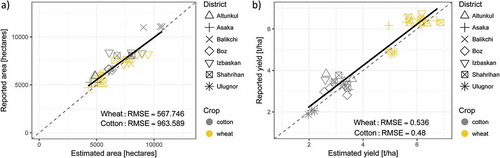
Regarding the yield modelling, the estimates were in good agreement with the official statistics. The LUE model yielded both under- and overestimation compared to the reported yields by approximatly 10% on average (over all districts with statistical data available). Irrespective of the crop type, the relationship between predicted and observed yields reached an R² of 0.812 for all crops. The strength of the relationship decreased when considering the crop types independently: the R² and RMSE were, respectively, 0.557 and 0.536 for wheat, and 0.631 and 0.480 for cotton.

Spatial pattern of cropland use intensity

The analysis of the indicators of cropland use intensity highlighted several spatial patterns. Cotton and wheat were cultivated throughout the landscape, whereas rice covered only minor parts of the valley (2–6%), preferably in its center (Figure 6). Overall, cotton was cultivated in the central and eastern parts of Fergana, and was often in rotation with wheat. Orchards were spread all over the area but occurred more frequently in the alluvial fans and the mountain slopes.

Figure 6. Maps for assessing cropland use intensity and productivity pattern (based on yield and water-use efficiency) at the field level.

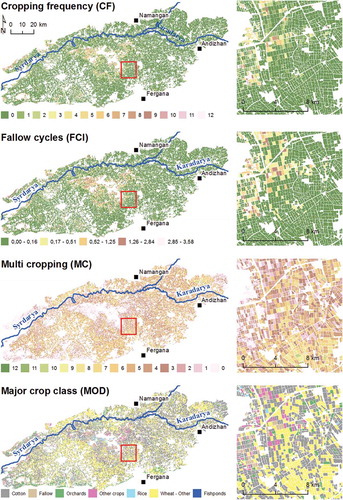
Figure 6. (Continued).

Cotton (2,235.38 km²; 34% of the cultivated area), wheat-other (1,876.64 km²; 29%), and orchards (1,407.87 km²; 22%) were the dominant crops in the Fergana Valley, which confirms the conclusions of Löw et al. (2013a). The annual crop maps and statistics indicate that the area of cotton and wheat-other, which covered a major part of Fergana Valley, displayed the most fluctuations in area across years. It is worth noting that these classes were mapped with high accuracy (>0.9; Table 3) which provides confidence in the changes in their corresponding planted area. The area of orchards appeared relatively constant over time, which highlights the reliability of the classification, as orchards are multiannual crops. Around 80% of the fields were cultivated every year. Overall, 3% of the agricultural fields had five–eight cropped years cropped and 92% of the fields even had high cropping frequencies (i.e., 9–11 years). Fields with a low cropping frequency presumably occurred in the central parts of the Fergana Valley and covered less than 5%. The fallow cycle maps showed that 16% of the cropland had at least one out of three fallow cycles. Two percent of the fields had a high fallow periodicity, which occurred mostly in the central parts of Fergana.

Assessing the annual crop maps from 2004–2014 revealed that double cropping was a widespread practice (Table 4). About 84% of the fields were cultivated with wheat-other (i.e., double-cropped) at least once during 2004–2014. Fields with 9–11 double-cropped years totalled to only 2% and were scattered all over the valley.

Table 4. Crop class statistics in Fergana Valley. Cultivated area per crop class are given in square kilometres. Statistics were derived from annual crop maps.

Year	Crop class (km^2)
	Fallow	Cotton	Rice	Other	Orchard	Winter wheat – Other	Water
2004	291.06	2387.71	348.8	183.82	1339.63	1795.51	15.61
2005	232.8	2363.48	457.22	242.07	1343.79	1707.27	15.52
2006	259.54	2523.62	123.24	227.82	1325.08	1887.33	15.52
2007	285.26	1957.95	661.85	175.6	1333.97	1931.91	15.61
2008	454.55	2225.54	181.5	341.5	1355.71	1787.84	15.52
2009	265.57	1495.41	570.48	239.75	1350.17	2425.24	15.52
2010	169.32	2294.58	193.89	344.48	1364.51	1979.86	15.52
2011	336.81	2451.2	125.02	239.09	1378.22	1815.97	15.84
2012	172.53	2563.05	198.99	379.29	1361.25	1671.28	15.78
2013	227.59	1948.27	631.63	289.11	1364.9	1880.27	20.38
2014	253.97	2378.35	239.89	323.12	1385.09	1760.54	21.19
Median	259.54	2363.48	239.89	242.07	1355.71	1815.97	15.61
Average	268.09	2235.38	339.32	271.42	1354.76	1876.64	16.55
Standard deviation	78.97	317.43	206.19	68.22	18.42	204.28	2.11

Spatial patterns of crop productivity

The deviation of crop yields from the estimated regional average yields (Figure 6) displayed two patterns. First, crop yields exhibited a high degree of heterogeneity, often with more than a two-fold difference, even at short distances. Second, lower yields tended to occur in the central parts of the Fergana Valley, where average deviations amounted to 10% and even reached 40%. Cotton displayed a broader distribution than wheat, with fields achieving more than 200% of average yield. The most productive cotton and wheat fields achieved 229% and 190% of the long-year median yields (2004–2014), respectively. However, this applied for less than 1% of all fields. Overall, the spatial patterns of water-use efficiency and crop yield were similar.

Identifying regions with similar productivity characteristics

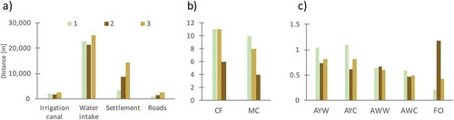
Three regions of distinct properties regarding cropping intensity and productivity were identified based on clustering (Figure 7). The first region covered 35.4% of the cropped area(excluding fields where cotton and wheat were never cultivated) and was characterized by a relatively high productivity – 104% and 109% cotton and wheat yield of the regional long-term average, respectively. Both the water-use efficiency and the cropping frequency were the highest observed. At the same time, fields belonging to this region tended to be closer to irrigation infrastructure and markets, as indicated by a low median distance (Figure 7).

Figure 7. Homogeneous regions (clusters) with similar cropping intensity and productivity properties, based on the portioning-around-medoids clustering. Clustering was not performed for those fields never planted with cotton or winter wheat.

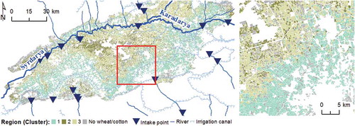
Whilst productivity in the third region (54.9% of all fields) tended to be in between the other two regions (Figure 8), the second region was characterized by comparatively low productivity (9.7% of observed fields). Average yields of wheat and cotton were only 73% and 61%, respectively, of the regional, long-term average. It occurred presumably in the central parts of the Fergana Valley, where distances to irrigation infrastructure and markets were high (Figure 8).

Figure 8. For three regions (clusters, see Figure 7), (a) distances to irrigation canals, intake points, settlements, and roads; (b) CF = cropping frequency, MC = multi cropping; (c) median values for AYW/AYC = average attainable yield for wheat/cotton, AWW/AWC = average water-use efficiency for wheat/cotton (Table 1), FCI = fallow cycles. Colours of the bars correspond to clusters in Figure 7.

Discussion and perspectives

Generalization potential of the method

This study established that fused time series of different satellite images (MODIS and Landsat) allowed capitalizing on the spatial resolution of Landsat while ensuring a high observation frequency with MODIS (R² ranging from 0.794 to 0.907). Thus, data fusion could be a suitable means to mitigate the inherent trade-off between spatial and temporal resolution in remote sensing-based agricultural monitoring (Atzberger 2013). This is especially critical when implementing an operational system as the data flow has to be sustained. From a crop mapping point of view, Landsat imagery is well-suited for inventory of crop types in agro-ecosystems characterized by fields of 6.7 ha on average, as observed in the Fergana Valley (Löw and Duveiller 2014). Its 16-day revisit-cycle, however, generally lengthened by cloud contamination, can jeopardize the high spatial resolution benefit of Landsat images for crop monitoring, and lead to classification uncertainty (Löw et al. 2013a). In contrast, MODIS has a high revisit frequency, but its coarse spatial resolution can limits its application to monitoring of large fields only (Duveiller, Baret, and Defourny 2011; Löw and Duveiller 2014), especially in fragmented landscapes (Waldner and Defourny 2017).

Compared to previous studies in Fergana (Löw et al. 2017a), the data fusion enabled assessing crop productivity over a long period due to creating a regular and high-resolution time series. This research provides the first continuous assessment at the field level in Fergana. At synoptic scale, the cropping patterns were in agreement with those found in previous studies, even though they mostly focused on 1–4 years only (Conrad et al. 2013b; Löw et al. 2017b; Löw et al. 2013a). Further, the accuracy of the crop maps was comparable or higher than other object-based crop classifications in Central Asia (Basukala et al. 2017; Löw et al. 2015b; Löw, Knöfel, and Conrad 2015c) and other regions (Balaguer et al. 2010; Duro, Franklin, and Dubé 2012). Whilst in the future, errors in the maps are likely to be reduced by incorporating more in-situ data for the training of the classifiers (e.g., Rodriguez-Galiano et al. 2012; Waske et al. 2010) or achieving a better balance in the training class proportion (Waldner, Jacques, and Löw 2017), the current low error rates offered already much prospective for an accurate crop type monitoring, and provide a suitable basis for yield and WUE estimation.

The accuracy of yield estimates suggests that the light-use efficiency model provided realistic information on the spatial variability in the region. Long-term average crop yields of cotton (3.04 t/ha) and wheat (4.65 t/ha) were in the range of other studies in Central Asia (Abdullaev et al. 2009b; Reddy 2012; SIC-ICWC (2016)). Deviations between estimated and reported yield statistics were in the range of previous attempts (Shi et al. 2007; Fritsch 2013; Lobell et al. 2003; Reeves, Zhao, and Running 2005). Further, Doraiswamy et al. (2005) and Alganci et al. (2014) reported a 10% deviation (compared to county-yield statistics) using a crop growth simulation model for corn and soybean, and a LUE model for cotton, respectively.

Overall, a high crop classification accuracy in combination with relatively low uncertainties in the yield estimates demonstrates the suitability of the combined use of satellite image time series and light-use efficiency models for assessing agricultural production. The operational advantage of the approach is the relatively low requirement of input parameters compared to approaches that apply crop simulation models.

Spatial patterns of productivity

Homogeneous regions in terms of crop intensity and productivity were identified based on clustering. Areas closer to intake points (regions 1 and 3, respectively) tended to have persistently higher crop yields and water-use efficiency. Higher crop yields (up to 10% higher than regional average) and cropping intensities presumably occurred in areas with a shorter distance to irrigation canals and were doubly cropping was frequent (especially region 1), while lower yields occur in areas with a higher distance to irrigation canals (especially region 2). Tail-end locations within the canal network in Central Asia usually are less endowed with water than head-end fields, which in turn lowers crop yields (Ruecker et al. 2012). This underlines the importance of differential access to irrigation water at head- and tail-end locations in an irrigation network (Conrad et al. 2013a). Likewise, agricultural production in region 2 appeared to be under water deficits and/or low application efficiencies, as water-use efficiency was lowest and the number of fallow cycles highest. It conforms a study on smaller scale in the south Fergana Valley canal region, where fluctuations in water delivery rates were higher in locations with a higher distance from the water intake points, i.e. in tail end locations (Abdullaev et al. 2009b). Likewise, disparities of water-use efficiency in region 2 was higher (standard deviation across wheat fields: 36%, cotton: 10%) than in region 1 (12% and 7%, respectively), which indicates that infrastructure deterioration and location within the irrigation system are major limiting factors of crop productivity, as reportedly considered in Central Asia (Abdullaev et al. 2009b; Cai, McKinney, and Rosegrant 2003). Small-scale fluctuations of crop yield, which can be in the range of 1 t/ha for neighbouring fields, can be understood in terms of variability within districts (Ruecker et al. 2012; Shi et al. 2007). In “dryer” years (2008, 2009 or 2014), the crop yield for cotton tended to be lower. Such a trend for wheat did not emerge because it generally requires less water to complete its cycle (Bekchanov, Karimov, and Lamers 2010).

Higher distances to settlements and roads are likely to cause another major constraint for maintaining the irrigation network. Factors related to market accessibility were partly more influencing than the status of irrigation infrastructure. This was indicated by the fact that despite fields in region two tended to be closer to canals (1,607 m) and intake points (21,246 m) than in region 1 (1,941 m and 22,575 m, respectively; Figure 7). This is likely to reflect the inability (e.g. due to financial constraints) to maintain the canal infrastructure, specifically in remote areas and also caused by low technical efficiencies of the production technologies (Karimov and Niño-Zarazúa 2014). Options for improving these technical efficiencies are determined by region, crop growing area, location and soil fertility. The results underline that yield could be increased by roughly 1.0 and 1.4 t/ha for cotton and wheat, respectively, if the access to water in region 2 reaches the same level as in region 1.

Limitations and perspectives

Several limitations of the system need to be considered when interpreting its outputs. First, the map uncertainty might be distributed unequally (Loosvelt et al. 2012b; Löw, Knöfel, and Conrad 2015c; Radoux et al. 2010), although the classification accuracy of the classes fallow, cotton, and wheat-other was high. A direct validation of the cropping indicators remains challenging because it would require retrospective reference data at the field-level for every year. Second, crop yield estimates were validated with aggregated statistics and deviations at the field level tend to be higher than those reported at the district level (Biradar et al. 2008; Platonov et al. 2008). In addition, within-field variations of crop types, which in rare occasions can occur, or crop yield are not represented in the maps and remains a challenge for yield gap analysis (Sadras et al. 2015).

This study facilitated the identification yield-limiting factors and might be used as baseline for guiding mitigating them in the future (Lobell 2013; Löw et al. 2017a). This in turn is a prerequisite to target ground efforts and identify opportunities for improving productivity and subsequently farmers’ income. Water-management organizations may now use this information to identify water saving opportunities, enhance productivity, or assess the effectiveness of water distribution (Reddy 2012).

Agricultural indicators still need to find their way into practice. They are at best provided as digital and openly accessible maps for land and water resource managers, or local and regional authorities and agencies. Further, such information must be provided at the field level and over time to continuously trace productivity, identify cold/hot spots productivity or regions threatened by frequent water scarcity, and finally measure target compliance, e.g., not only by policy and management decisions but also according to sustainable development goals (United Nations 2016). To fulfil this purpose, all the maps produced are available through an online tool that is being developed for Central Asia (http://geoagro.icarda.org/en/gis/details/index).

Conclusions

In Central Asia, closing the yield gap while improving the water-use efficiency is one of the chief challenges of the next decades. Better knowledge of the dynamics and spatial patterns of cropland use intensity and productivity as well as their limiting factors would support decision-making. The overarching objective was to develop a method to achieve annual and multi-annual assessment of agricultural production in the Fergana Valley, Uzbekistan. To ensure reliability, timeliness and accuracy, particular attention was paid to implement an approach with minimum calibration data requirements and sustained remotely sensed data flows. Fused time series of MODIS and Landsat images were produced to provide the high frequency gapless 30-m data required for crop classification, yield, and water-use efficiency estimation. Per-field indicators of cropland use efficiency and productivity were then derived. Results exhibited good agreement with reported crop areas and yields across Fergana. As archive satellite data allows hindcasting dynamics of agricultural productivity, the identification of spatial patterns of cropping intensity and productivity became possible. Such maps could not only serve as baseline to identify regions for intensifying agriculture, but also to regions potentially affected by land degradation or irrigation infrastructure deterioration, which entails to equip agricultural managers and decision makers with knowledge of the most important indicators of agricultural productivity, and their constraining factors. Results demonstrated that remotely sensed estimates of agricultural productivity could provide a unique perspective that would enhance the ability to identify management priorities for improving regional production and/or reducing environmental impacts. This work settles the ground for the transition of satellite-driven crop monitoring from research to operations with minimum calibration data requirements. The proposed approach could be implemented in other irrigated regions in a cost-effective fashion, by adapting regional meteorological and crop-specific parameters.

Highlights

• Implemented the first earth observation-based monitoring for tracking dynamics of agricultural productivity in the Fergana Valley at the field level

• Provided maps about land use, crop yield, and water-use efficiency annually and synthetized in multi-year metrics for the first time

• Identified regions with similar land-use intensity and productivity characteristics using clustering techniques

• Found agricultural productivity impacted by the status of irrigation infrastructure and distance of fields to markets

• Provided management options for improving crop production in regions characterized by low productivity

Acknowledgements

We would like to express our sincere gratitude to Prof. Dr Victor Dukhovny and Dr Galina Stulina (SIC-ICWC) for providing data (water inflow and reference data) and profound feedback to this study. Further, we thank the various reviewers for their valuable work on bringing the article into its present form.

Disclosure statement

No potential conflict of interest was reported by the authors.

References

- Abbas, A., S. Khan, N. Hussain, M. A. Hanjra, and S. Akbar. 2010. “Characterizing Soil Salinity in Irrigated Agriculture Using a Remote Sensing Approach.” Physical Chemical Earth, Parts A/B/C 55 43–52.
- Abdullaev, I., C. De Fraiture, M. Giordano, M. Yakubov, and A. Rasulov. 2009a. “Agricultural Water Use and Trade in Uzbekistan: Situation and Potential Impacts of Market Liberalization.” International Journal Water Resources Developments 25: 47–63. doi:10.1080/07900620802517533.
- Abdullaev, I., J. Kazbekov, K. Jumaboev, and H. Manthritilake. 2009b. “Adoption of Integrated Water Resources Management Principles and Its Impacts: Lessons from Ferghana Valley.” Water International 34: 230–241. doi:10.1080/02508060902843710.
- Alcantara, C., T. Kuemmerle, A. V. Prishchepov, and V. C. Radeloff. 2012. “Mapping Abandoned Agriculture with Multi-Temporal MODIS Satellite Data.” Remote Sens Environment 124: 334–347. doi:10.1016/j.rse.2012.05.019.
- Alexandratos, N., and J. Bruinsma. 2012. World Agriculture: Towards 2030/2050 - The 2012 Revision (Report). Rome: FAO.
- Alganci, U., M. Ozdogan, E. Sertel, and C. Ormeci. 2014. “Estimating Maize and Cotton Yield in Southeastern Turkey with Integrated Use of Satellite Images, Meteorological Data and Digital Photographs.” F Crop Researcher 157: 8–19. doi:10.1016/j.fcr.2013.12.006.
- Allen, R. P., L. S. Pereira, D. Raes, and M. Smith, 1998. Crop Evapotranspiration Guidelines for Computing Crop Water Requirements. FAO Irrig. Drain. Pap. 56, FAO United Nations 56.
- Aslan, S. T., and K. S. Gundoglu. 2007. “Mapping Multi-Year Groundwater Depth Patterns from Time-Series Analyses of Seasonally Lowest Depth-To-Groundwater Maps in Irrigation Areas.” Polish Journal Environment Studies 16: 183–190.
- Atzberger, C. 2013. “Advances in Remote Sensing of Agriculture: Context Description, Existing Operational Monitoring Systems and Major Information Needs.” Remote Sens 5: 949–981. doi:10.3390/rs5020949.
- Bahçeci, I., N. Dinç, A. F. Tari, A. I. Aǧar, and B. Sönmez. 2006. “Water and Salt Balance Studies, Using SaltMod, to Improve Subsurface Drainage Design in the Konya-ÇUmra Plain, Turkey.” Agricultural Water Managed 85: 261–271. doi:10.1016/j.agwat.2006.05.010.
- Balaguer, A., L. A. Ruiz, T. Hermosilla, and J. A. Recio. 2010. “Definition of a Comprehensive Set of Texture Semivariogram Features and Their Evaluation for Object-Oriented Image Classification.” Computation Geosci 36: 231–240. doi:10.1016/j.cageo.2009.05.003.
- Bastiaanssen, W. G. M., D. J. Molden, and I. W. Makin. 2000. “Remote Sensing for Irrigated Agriculture: Examples from Research and Possible Applications.” Agricultural Water Managed 46: 137–155. doi:10.1016/S0378-3774(00)00080-9.
- Bastiaanssen, W. G. M., and M. G. Bos. 1999. “Irrigation Performance Indicators Based on Remotely Sensed Data: A Review of Literature.” Irrig Drain Systems 13: 291–311. doi:10.1023/A:1006355315251.
- Bastiaanssen, W. G. M., and N. R. Harshadeep. 2005. “Managing Scarce Water Resources in Asia: The Nature of the Problem and Can Remote Sensing Help?.” Irrig Drain Systems 19: 269–284. doi:10.1007/s10795-005-5188-y.
- Basukala, A. K., C. Oldenburg, J. Schellberg, M. Sultanov, and O. Dubovyk. 2017. “Towards Improved Land Use Mapping of Irrigated Croplands: Performance Assessment of Different Image Classification Algorithms and Approaches.” European Journal Remote Sens 50: 187–201. doi:10.1080/22797254.2017.1308235.
- Bekchanov, M., A. Karimov, and J. P. A. Lamers. 2010. “Impact of Water Availability on Land and Water Productivity: A Temporal and Spatial Analysis of the Case Study Region Khorezm, Uzbekistan.” Water 2: 668–684. doi:10.3390/w2030668.
- Bichsel, C. 2009. Conflict Transformation in Central Asia - Irrigation Disputes in the Ferghana Valley. Taylor & Francis eLibrary.
- Biradar, C. M., P. S. Thenkabail, A. Platonov, X. Xiao, R. Geerken, P. Noojipady, H. Turral, and J. Vithanage. 2008. “Water Productivity Mapping Methods Using Remote Sensing.” Journal Applications Remote Sens 2: 23544. doi:10.1117/1.3033753.
- Bolton, D. K., and M. A. Friedl. 2013. “Forecasting Crop Yield Using Remotely Sensed Vegetation Indices and Crop Phenology Metrics.” Agricultural Forest Meteorol 173: 74–84. doi:10.1016/j.agrformet.2013.01.007.
- Breiman, L. 2001. “Random Forests.” Mach Learning 45: 5–32. doi:10.1023/A:1010933404324.
- Cai, X., D. Molden, M. Mainuddin, B. Sharma, M.-D. Ahmad, and P. Karimi. 2011. “Producing More Food with Less Water in a Changing World: Assessment of Water Productivity in 10 Major River Basins.” Water International 36: 42–62. doi:10.1080/02508060.2011.542403.
- Cai, X., D. C. McKinney, and M. W. Rosegrant. 2003. “Sustainability Analysis for Irrigation Water Management in the Aral Sea Region.” Agricultural Systems 76: 1043–1066. doi:10.1016/S0308-521X(02)00028-8.
- Chen, J., P. Jönsson, M. Tamura, Z. Gu, B. Matsushita, and L. Eklundh. 2004. “A Simple Method for Reconstructing a High-Quality NDVI Time-Series Data Set Based on the Savitzky–Golay Filter.” Remote Sens Environment 91: 332–344. doi:10.1016/j.rse.2004.03.014.
- Chen, J., X. Zhu, J. E. Vogelmann, F. Gao, and S. Jin. 2011. “A Simple and Effective Method for Filling Gaps in Landsat ETM+ SLC-off Images.” Remote Sens Environment 115: 1053–1064. doi:10.1016/j.rse.2010.12.010.
- Chiang, M. M. T., and B. Mirkin. 2010. “Intelligent Choice of the Number of Clusters in K-Means Clustering: An Experimental Study with Different Cluster Spreads.” Journal Classif 27: 3–40. doi:10.1007/s00357-010-9049-5.
- Christmann, S., Martius, C., Bedoshvili, D., Bobojonov, I., Carli, C., Devkota, K., Ibragimov, Z. & Mavlyanova, R., 2009. Food security and climate change in Central Asia and the Caucasus. CGIAR-PFU, ICARDA, Tashkent, Uzbekistan, 75.
- Congalton, R. G. 1991. “A Review of Assessing the Accuracy of Classifications of Remotely Sensed Data.” Remote Sens Environment 37: 35–46. doi:10.1016/0034-4257(91)90048-B.
- Conrad, C., M. Rahmann, M. Machwitz, G. Stulina, H. Paeth, and S. Dech. 2013b. “Satellite Based Calculation of Spatially Distributed Crop Water Requirements for Cotton and Wheat Cultivation in Fergana Valley, Uzbekistan.” Glob Planet Change 110: 88–98. doi:10.1016/j.gloplacha.2013.08.002.
- Conrad, C., S. W. Dech, M. Hafeez, J. P. A. Lamers, and B. Tischbein. 2013a. “Remote Sensing and Hydrological Measurement Based Irrigation Performance Assessments in the Upper Amu Darya Delta, Central Asia.” Physical Chemical Earth, Parts A/B/C 61–62 52–62. doi:10.1016/j.pce.2013.05.002.
- Cortes, C., and V. Vapnik. 1995. “Support-Vector Networks.” Mach Learning 20: 273–297. doi:10.1007/BF00994018.
- de Beurs, K. M., and G. Ioffe. 2014. “Use of Landsat and MODIS Data to Remotely Estimate Russia’s Sown Area.” Journal Land Use Sciences 9: 377–401. doi:10.1080/1747423X.2013.798038.
- de Leeuw, J., A. Vrieling, A. Shee, C. Atzberger, K. M. Hadgu, C. M. Biradar, H. Keah, and C. Turvey. 2014. “The Potential and Uptake of Remote Sensing in Insurance: A Review.” Remote Sens 6: 10888–10912. doi:10.3390/rs61110888.
- Doraiswamy, P., J. Hatfield, B. Jackson, B. Akhmedov, J. Prueger, and A. Stern. 2004. “Crop Condition and Yield Simulations Using Landsat and MODIS.” Remote Sens Environment 92: 548–559. doi:10.1016/j.rse.2004.05.017.
- Doraiswamy, P. C., T. R. Sinclair, S. Hollinger, B. Akhmedov, A. Stern, and J. Prueger. 2005. “Application of MODIS Derived Parameters for Regional Crop Yield Assessment.” Remote Sens Environment 97: 192–202. doi:10.1016/j.rse.2005.03.015.
- Dregne, H. E. 2002. “Land Degradation in the Drylands.” Arid L Researcher Managed 16: 99–132. doi:10.1080/153249802317304422.
- Dubovyk, O., G. Menz, C. Conrad, E. Kan, M. Machwitz, and A. Khamzina. 2013. “Spatio-Temporal Analyses of Cropland Degradation in the Irrigated Lowlands of Uzbekistan Using Remote-Sensing and Logistic Regression Modeling.” Environment Monitoring Assessment 185: 4775–4790. doi:10.1007/s10661-012-2904-6.
- Duro, D. C., S. E. Franklin, and M. G. Dubé. 2012. “A Comparison of Pixel-Based and Object-Based Image Analysis with Selected Machine Learning Algorithms for the Classification of Agricultural Landscapes Using SPOT-5 HRG Imagery.” Remote Sens Environment 118: 259–272. doi:10.1016/j.rse.2011.11.020.
- Duveiller, G. 2011. Crop Specific Green Area Index Retrieval from Multi-Scale Remote Sensing for Agricultural Monitoring. Université catholique de Louvain. Louvain-la-Neuve: Belgium.
- Duveiller, G., F. Baret, and P. Defourny. 2011. “Crop Specific Green Area Index Retrieval from MODIS Data at Regional Scale by Controlling Pixel-Target Adequacy.” Remote Sens Environment 115: 2686–2701. doi:10.1016/j.rse.2011.05.026.
- Estel, S., T. Kuemmerle, C. Alcantara, C. Levers, A. V. Prishchepov, P. Hostert, C. Alcántara, et al. 2015. “Mapping Farmland Abandonment and Recultivation across Europe Using MODIS NDVI Time Series.” Remote Sens Environment 163: 312–325. doi:10.1016/j.rse.2015.03.028.
- Estel, S., T. Kuemmerle, C. Levers, M. Baumann, and P. Hostert. 2016. “Mapping Cropland-Use Intensity across Europe Using MODIS NDVI Time Series.” Environment Researcher Letters 11: 24015. doi:10.1088/1748-9326/11/2/024015.
- Fawcett, T. 2006. “An Introduction to ROC Analysis.” Pattern Recognit Letters 27: 861–874. doi:10.1016/j.patrec.2005.10.010.
- Fischer, G., H. Van Velthuizen, M. Shah, and F. Nachtergaele. 2002. Global Agro-Ecological Assessment for Agriculture in the 21st Century : Methodology and Results. Laxenburg: International Institute for Applied Systems Analysis.
- Foody, G. M. 2009. “Classification Accuracy Comparison: Hypothesis Tests and the Use of Confidence Intervals in Evaluations of Difference, Equivalence and Non-Inferiority”. Remote Sens Environment 113: 1658–1663. 10.1016/j.rse.2009.03.014
- Fritsch, S., 2013. Spatial and temporal patterns of crop yield and marginal land in the Aral Sea Basin: derivation by combining multi-scale and multi-temporal remote sensing data with a light use efficiency model (PhD Thesis). University of Wuerzburg.
- Gao, F., Masek, J., Schwaller, M., & F. Hall. 2006. “On the Blending of the MODIS and Landsat ETM + Surface Reflectance.” IEEE Transactions on Geoscience and Remote Sensing: 44(8), 2207–2218
- Gibbs, H. K., and J. M. Salmon. 2015. “Mapping the World’s Degraded Lands.” Applications Geographic 57: 12–21. doi:10.1016/j.apgeog.2014.11.024.
- González-Dugo, M. P., and L. Mateos. 2008. “Spectral Vegetation Indices for Benchmarking Water Productivity of Irrigated Cotton and Sugarbeet Crops.” Agricultural Water Managed 95: 48–58. doi:10.1016/j.agwat.2007.09.001.
- Haboudane, D., J. R. Miller, N. Tremblay, P. Zarco-Tejada, and L. Dextraze. 2002. “Integrated Narrow-Band Vegetation Indices for Prediction of Crop Chlorophyll Content for Application to Precision Agriculture.” Remote Sens Environment 81: 416–426. doi:10.1016/S0034-4257(02)00018-4.
- Horst, M. G., S. S. Shamutalov, L. S. Pereira, and J.M. Gonçalves. 2005. “Field Assessment Of The Water Saving Potential With Furrow Irrigation In Fergana, Aral Sea Basin.” Agricultural Water Management 77 (1): 210-231. doi:10.1016/j.agwat.2004.09.041.
- Hunink, J. E., and P. Droogers. 2011. Climate Change Impact Assessment on Crop Production in Uzbekistan. Wageningen.
- Hüttich, C., M. Herold, M. Wegmann, A. Cord, B. Strohbach, C. Schmullius, and S. Dech. 2011. “Assessing Effects of Temporal Compositing and Varying Observation Periods for Large-Area Land-Cover Mapping in Semi-Arid Ecosystems : Implications for Global Monitoring.” Remote Sens Environment 115: 2445–2459. doi:10.1016/j.rse.2011.05.005.
- Ibrakhimov, M., A. Khamzina, I. Forkutsa, G. Paluasheva, J. P. A. Lamers, B. Tischbein, P. L. G. Vlek, and C. Martius. 2007. “Groundwater Table and Salinity: Spatial and Temporal Distribution and Influence on Soil Salinization in Khorezm Region (Uzbekistan, Aral Sea Basin).” Irrig Drain Systems 21: 219–236. doi:10.1007/s10795-007-9033-3.
- IIASA, FAO, 2012. Global Agro-Ecological Zones (GAEZ V3.0) [WWW Document].
- Jacquin, A., D. Sheeren, and J. Lacombe. 2010. “Vegetation Cover Degradation Assessment in Madagascar Savanna Based on Trend Analysis of MODIS NDVI Time Seriese.” International Journal Applications Earth Obs Geoinf 12: 3–10. doi:10.1016/j.jag.2009.11.004.
- Jarihani, A. A., T. R. McVicar, T. G. van Niel, I. V. Emelyanova, J. N. Callow, and K. Johansen. 2014. “Blending Landsat and MODIS Data to Generate Multispectral Indices: A Comparison of “Index-Then-Blend” and “Blend-Then-Index” Approaches.” Remote Sens 6: 9213–9238. doi:10.3390/rs6109213.
- Johnson, D. M. 2014. “An Assessment of Pre- and Within-Season Remotely Sensed Variables for Forecasting Corn and Soybean Yields in the United States.” Remote Sens Environment 141: 116–128. doi:10.1016/j.rse.2013.10.027.
- Jonsson, P., and L. Eklundh. 2004. “A Program for Analyzing Time-Series of Satellite Sensor Data.” Computation Geosci 30: 833–845. doi:10.1016/j.cageo.2004.05.006.
- Karimov, A., and M. Niño-Zarazúa. 2014. “Assessing Efficiency of Input Utilization in Wheat Production in Uzbekistan.” In: Restructuring Land Allocation, Water Use and Agricultural Value Chains. Technologies, Policies and Practices for the Lower Amudarya Region, Eds. J. P. A. Lamers, A. Khamzina, I. Rudenko, and P. L. G. Vlek, 231–252, Bonn: Bonn University Press.
- Kaufman, L., and P. J. Rousseeuw, 1990. Finding Groups in Data: An Introduction to Cluster Analysis (Wiley Series in Probability and Statistics), Eepe.Ethz.Ch.
- Knauer, K., Gessner, U., Fensholt, R., & Kuenzer, C. (2016). An ESTARFM fusion framework for the generation of large-scale time series in cloud-prone and heterogeneous landscapes. Remote Sensing, 8(5), 425.
- Kuemmerle, T., K. Erb, P. Meyfroidt, D. Müller, P. H. Verburg, S. Estel, H. Haberl, et al. 2013. “Challenges and Opportunities in Mapping Land Use Intensity Globally.” Current Opinion Environment Sustain 5: 484–493. doi:10.1016/j.cosust.2013.06.002.
- Kussul, N., S. Skakun, A. Shelestov, O. Kravchenko, J. F. Gallego, and O. Kusul. 2012. “Crop Area Estimation in Ukraine Using Satellite Data within the MARS Project.” In Geoscience and Remote Sensing Symposium (IGARSS), 2012 IEEE International, July 22-27 . 3756–3759.
- Latchininsky, A. V. 2013. “Locusts and Remote Sensing: A Review.” Journal of Applied Remote Sensing 7(1), 1-32. doi:10.1117/1.JRS.7.075099.
- Lex, S., S. Asam, F. Löw, and C. Conrad. 2015. “Comparison of Two Statistical Methods for the Derivation of the Fraction of Absorbed Photosynthetic Active Radiation for Cotton.” Photogramm - Fernerkundung - Geoinformation 2015: 55–67. doi:10.1127/pfg/2015/0250.
- Li, L., M. A. Friedl, Q. Xin, J. Gray, Y. Pan, and S. Frolking. 2014. “Mapping Crop Cycles in China Using MODIS-EVI Time Series.” Remote Sens 6: 2473–2493. doi:10.3390/rs6032473.
- Li, W., M. Weiss, F. Waldner, P. Defourny, V. Demarez, D. Morin, O. Hagolle, and F. Baret. 2015. “A Generic Algorithm to Estimate LAI, FAPAR and FCOVER Variables from SPOT4_HRVIR and Landsat Sensors: Evaluation of the Consistency and Comparison with Ground Measurements.” Remote Sens 7: 15494–15516. doi:10.3390/rs71115494.
- Liu, J., E. Pattey, J. R. Miller, H. McNairn, A. Smith, and B. Hu. 2010. “Estimating Crop Stresses, Aboveground Dry Biomass and Yield of Corn Using Multi-Temporal Optical Data Combined with a Radiation Use Efficiency Model.” Remote Sens Environment 114: 1167–1177. doi:10.1016/j.rse.2010.01.004.
- Lobell, D. B. 2013. “The Use of Satellite Data for Crop Yield Gap Analysis.” F Crop Researcher 143: 56–64. doi:10.1016/j.fcr.2012.08.008.
- Lobell, D. B., D. Thau, C. Seifert, E. Engle, and B. Little. 2015. “A Scalable Satellite-Based Crop Yield Mapper.” Remote Sens Environment 164: 324–333. doi:10.1016/j.rse.2015.04.021.
- Lobell, D. B., G. P. Asner, J. I. Ortiz-Monasterio, and T. L. Benning. 2003. “Remote Sensing of Regional Crop Production in the Yaqui Valley, Mexico: Estimates and Uncertainties.” Agricultural Ecosyst Environment 94: 205–220. doi:10.1016/S0167-8809(02)00021-X.
- Lobell, D. B., J. I. Ortiz-Monasterio, and A. S. Lee. 2010. “Satellite Evidence for Yield Growth Opportunities in Northwest India.” F Crop Researcher 118: 13–20. doi:10.1016/j.fcr.2010.03.013.
- Lobell, D. B., J. I. Ortiz-Monasterio, G. P. Asner, R. L. Naylor, and W. P. Falcon. 2005. “Combining Field Surveys, Remote Sensing, and Regression Trees to Understand Yield Variations in an Irrigated Wheat Landscape.” Agronomic Journal 97: 241–249.
- Lobell, D. B., K. G. Cassman, C. B. Field, and C. B. Field. 2009. “Crop Yield Gaps: Their Importance, Magnitudes, and Causes.” Annual Reviews Environment Resources 34: 179–204. doi:10.1146/annurev.environ.041008.093740.
- Loosvelt, L., J. Peters, and H. Skriver. 2012a. “Impact of Reducing Polarimetric SAR Input on the Uncertainty of Crop Classifications Based on the Random Forests Algorithm.” IEEE Transactions Geosci Remote Sens 50: 4185–4200. doi:10.1109/TGRS.2012.2189012.
- Loosvelt, L., J. Peters, H. Skriver, H. Lievens, F. M. B. van Coillie, B. de Baets, and N. E. C. Verhoest. 2012b. “Random Forests as a Tool for Estimating Uncertainty at Pixel-Level in SAR Image Classification.” International Journal Applications Earth Obs Geoinf 19: 173–184. doi:10.1016/j.jag.2012.05.011.
- Löw, F., C. Biradar, E. Fliemann, J. P. A. Lamers, and C. Conrad. 2017a. “Assessing Gaps in Irrigated Agricultural Productivity through Satellite Earth Observations — A Case Study of the Fergana Valley, Central Asia.” International Journal Applications Earth Obs Geoinf 59: 118–134. doi:10.1016/j.jag.2017.02.014.
- Löw, F., C. Conrad, and U. Michel. 2015a. “Decision Fusion and Non-Parametric Classifiers for Land Use Mapping Using Multi-Temporal RapidEye Data.” ISPRS Journal Photogramm Remote Sens 108: 191–204. doi:10.1016/j.isprsjprs.2015.07.001.
- Löw, F., E. Fliemann, A. Narvaez Vallejo, and C. Biradar. 2016a. Mapping Agricultural Production in the Fergana Valley Using Satellite Earth Observation - Project Report.
- Löw, F., E. Fliemann, I. Abdullaev, C. Conrad, and J. P. A. Lamers. 2015b. “Mapping Abandoned Agricultural Land in Kyzyl-Orda, Kazakhstan Using Satellite Remote Sensing.” Applications Geographic 8: 377–390. doi:10.1016/j.apgeog.2015.05.009.
- Löw, F., Waldner, F., Latchininsky, A., Biradar, C., Bolkart, M., & Colditz, R. R. (2016). Timely monitoring of Asian Migratory locust habitats in the Amudarya delta, Uzbekistan using time series of satellite remote sensing vegetation index. Journal of environmental management, 183, 562-575.
- Löw, F., F. Waldner, O. Dubovyk, A. Akramkhanov, C. Biradar, J. P. A. Lamers, and A. V. Prishchepov. 2017b. Mapping Abandoned Cropland in the Aral Sea Basin with MODIS Time Series (Under Review).
- Löw, F., and G. Duveiller. 2014. “Defining the Spatial Resolution Requirements for Crop Identification Using Optical Remote Sensing.” Remote Sens 6: 9034–9063. doi:10.3390/rs6099034.
- Löw, F., P. Knöfel, and C. Conrad. 2015c. “Analysis of Uncertainty in Multi-Temporal Object-Based Classification.” ISPRS Journal Photogramm Remote Sens 105: 91–106. doi:10.1016/j.isprsjprs.2015.03.004.
- Löw, F., P. Navratil, K. Kotte, H. F. Schöler, and O. Bubenzer. 2013b. “Remote Sensing Based Analysis of Landscape Change in the Desiccated Seabed of the Aral Sea - A Potential Tool for Assessing the Hazard Degree of Dust and Salt Storms.” Environment Monitoring Assessment 185: 8303–8319. doi:10.1007/s10661-013-3174-7.
- Löw, F., U. Michel, S. Dech, and C. Conrad. 2013a. “Impact of Feature Selection on the Accuracy and Spatial Uncertainty of Per-Field Crop Classification Using Support Vector Machines.” ISPRS Journal Photogramm Remote Sens 85: 102–119. doi:10.1016/j.isprsjprs.2013.08.007.
- Martinez-Casasnovas, J., A. Martín-Montero, and M. Auxiliadora Casterad. 2005. “Mapping Multi-Year Cropping Patterns in Small Irrigation Districts from Time-Series Analysis of Landsat TM Images.” European Journal Agronomic 23: 159–169. doi:10.1016/j.eja.2004.11.004.
- Matton, N., G. S. G. S. Canto, F. Waldner, S. Valero, D. Morin, J. Inglada, M. Arias, S. Bontemps, B. Koetz, and P. Defourny. 2015. “An Automated Method for Annual Cropland Mapping along the Season for Various Globally-Distributed Agrosystems Using High Spatial and Temporal Resolution Time Series.” Remote Sens 7: 13208–13232. doi:10.3390/rs71013208.
- McNemar, Q. 1947. “Note on the Sampling Error of the Difference between Correlated Proportions or Percentages.” Psychometrika 12: 153–157. doi:10.1007/BF02295996.
- Metternicht, G., and J. Zinck. 2003. “Remote Sensing of Soil Salinity: Potentials and Constraints.” Remote Sens Environment 85: 1–20. doi:10.1016/S0034-4257(02)00188-8.
- Micklin, P. 2016. “The Future Aral Sea: Hope and Despair.” Environment Earth Sciences 75: 1–15. doi:10.1007/s12665-016-5614-5.
- Molden, D., and R. Sakthivadivel. 1999. “Water Accounting to Assess Use and Productivity of Water.” International Journal Water Resources Developments 15: 55–71. doi:10.1080/07900629948934.
- Monteith, J. L., and C. J. Moss. 1977. “Climate and the Efficiency of Crop Production in Britain [And Discussion].” Philosophy Transactions R Social London B Biologic Sciences 281: 277–294. doi:10.1098/rstb.1977.0140.
- Munoz, G., and J. Grieser. 2006. CLIMWAT 2.0 For CROPWAT (Computer Program).
- Peña-Barragán, J. M., M. K. Ngugi, R. E. Plant, and J. Six. 2011. “Object-Based Crop Identification Using Multiple Vegetation Indices, Textural Features and Crop Phenology.” Remote Sens Environment 115: 1301–1316. doi:10.1016/j.rse.2011.01.009.
- Pereira, L. S., P. Paredes, E. D. Сholpankulov, O. P. Inchenkova, P. R. Teodoro, and M.G. Horst. 2009. “Irrigation Scheduling Strategies For Cotton To Cope With Water Scarcity In The Fergana Valley, Central Asia.” Agricultural Water Management 96 (5): 723-735. doi:10.1016/j.agwat.2008.10.013.
- Platonov, A., P. S. Thenkabail, C. M. Biradar, X. Cai, M. Gumma, V. Dheeravath, Y. Cohen, et al. 2008. “Water Productivity Mapping (WPM) Using Landsat ETM+ Data for the Irrigated Croplands of the Syrdarya River Basin in Central Asia.” Sensors 8: 8156–8180. doi:10.3390/s8128156.
- Policar, R. 2006. “Ensemble Based Systems in Decision Making.” IEEE Circuits Systems Mag 6: 21–45. doi:10.1109/MCAS.2006.1688199.
- Radoux, J., P. Bogaert, D. Fasbender, and P. Defourny. 2010. “Thematic Accuracy Assessment of Geographic Object-Based Image Classification.” International Journal Geographic Information Sciences 25: 1–17.
- Reddy, J. M. 2012. “Analysis of Cotton Water Productivity in Fergana Valley of Central Asia.” Agricultural Sciences 3: 822–834.
- Reddy, J. M., K. Jumaboev, B. Matyakubov, and D. Eshmuratov. 2013. “Evaluation Of Furrow Irrigation Practices In Fergana Valley Of Uzbekistan.” Agricultural Water Management 117: 133-144. doi:10.1016/j.agwat.2012.11.004.
- Reeves, M. C., M. Zhao, and S. W. Running. 2005. “Usefulness and Limits of MODIS GPP for Estimating Wheat Yield.” International Journal Remote Sens 26: 1403–1421. doi:10.1080/01431160512331326567.
- Renier, C., F. Waldner, D. Jacques, M. Babah Ebbe, K. Cressman, and P. Defourny. 2015. “A Dynamic Vegetation Senescence Indicator for Near-Real-Time Desert Locust Habitat Monitoring with MODIS.” Remote Sens 7: 7545–7570. doi:10.3390/rs70607545.
- Roberts, A. M., G. Park, A. R. Melland, and I. Miller. 2009. “Trialling a Web-Based Spatial Information Management Tool with Land Managers in Victoria, Australia.” Journal of Environmental Management 91: 523–531. doi:10.1016/j.jenvman.2009.09.021.
- Rodriguez-Galiano, V. F., B. Ghimire, J. Rogan, M. Chica-Olmo, and J. P. Rigol-Sanchez. 2012. “An Assessment of the Effectiveness of a Random Forest Classifier for Land-Cover Classification.” ISPRS Journal Photogramm Remote Sens 67: 93–104. doi:10.1016/j.isprsjprs.2011.11.002.
- Roerink, G. J., Z. Su, and M. Menenti. 2000. “S-SEBI: A Simple Remote Sensing Algorithm to Estimate the Surface Energy Balance.” Physical Chemical Earth, Particle B Hydrol Ocean Atmos 25: 147–157. doi:10.1016/S1464-1909(99)00128-8.
- Rouse, J. W., R. H. Haas, J. A. Schell, and D. W. Deering. 1974. “Monitoring Vegetation Systems in the Great Plains with ERTS.” In Proceedings of the Earth Resources Technology Satellite Symposium NASA SP-351, Eds. S. C. Freden, E. P. Mercanti, and M. A. Becker, 309−317. Washington, DC: NASA.
- Ruecker, G., C. Conrad, N. Ibragimov, K. Kienzler, M. Ibrakhimov, C. Martius, and J. Lamers. 2012. “Spatial Distribution of Cotton Yield and Its Relationship to Environmental, Irrigation Infrastructure and Water Management Factors on a Regional Scale in Khorezm, Uzbekistan.” In Cotton, Water, Salts and Soums: Economic and Ecological Restructuring in Khorezm, Eds. C. Martius, I. Rudenko, J. P. A. Lamers, and P. L. G. Vlek, 1–419. Uzbekistan: Springer.
- Sadras, V. O., K. G. G. Cassman, P. Grassini, A. J. Hall, W. G. M. Bastiaanssen, A. G. Laborte, A. E. Milne, G. Sileshi, and P. Steduto, 2015. Yield Gap Analysis of Field Crops, Methods and Case Studies. FAO Water Reports 41.
- Saiko, T. A., and I. S. Zonn. 2000. “Irrigation Expansion and Dynamics of Desertification in the Circum-Aral Region of Central Asia.” Applications Geographic 20: 349–367. doi:10.1016/S0143-6228(00)00014-X.
- Salmon, J. M., M. A. Friedl, S. Frolking, D. Wisser, and E. M. Douglas. 2015. “Global Rain-Fed, Irrigated, and Paddy Croplands: A New High Resolution Map Derived from Remote Sensing, Crop Inventories and Climate Data.” International Journal Applications Earth Obs Geoinf 38: 321–334. doi:10.1016/j.jag.2015.01.014.
- Sauer, T., P. Havlík, U. A. Schneider, E. Schmid, G. Kindermann, and M. Obersteiner. 2010. “Agriculture and Resource Availability in a Changing World: The Role of Irrigation.” Water Resources Researcher 46, N/A-N/A. doi:10.1029/2009WR007729.
- Sellers, P. J., D. A. Randall, G. J. Collatz, J. A. Berry, C. B. Field, D. A. Dazlich, C. Zhang, G. D. Collelo, and L. Bounoua. 1996. “A Revised Land Surface Parameterization (Sib2) for Atmospheric GCMs.” Particle I: Model Formulation Journal Climate 9: 676–705.
- Senay, G. B., S. Bohms, P. H. Singh, N. M. Gowda, H. Velpuri, H. Alemu, and J. Verdin. 2013. “Operational Evapotranspirationmapping Using Remote Sensing Andweather Datasets: A New Parameterization for the SSEB Approach.” Journal American Water Resources Association 49: 577–591. doi:10.1111/jawr.12057.
- Sepulcre-Cantóa, G., F. Gellens-Meulenberghsa, A. Arboleda, G. Duveiller, A. de Wit, H. Eerens, B. Djabye, and P. Defourny. 2013. “Estimating Crop-Specific Evapotranspiration Using Remote-Sensing Imagery at Various Spatial Resolutions for Improving Crop Growth Modelling.” International Journal Remote Sens 34: 3274–3288. doi:10.1080/01431161.2012.716911.
- Shao, Y., R. S. Lunetta, J. Ediriwickrema, and J. Liames. 2009. “Mapping Cropland and Major Crop Types across the Great Lakes Basin Using MODIS-NDVI Data.” Photogramm Engineering Remote Sensing 76: 73–84. doi:10.14358/PERS.76.1.73.
- Shi, Z., G. R. Ruecker, M. Mueller, C. Conrad, N. Ibragimov, J. P. A. Lamers, C. Martius, G. Strunz, S. Dech, and P. L. G. Vlek. 2007. “Modeling of Cotton Yields in the Amu Darya River Floodplains of Uzbekistan Integrating Multitemporal Remote Sensing and Minimum Field Data.” Agronomic Journal 99: 1317–1326. doi:10.2134/agronj2006.0260.
- SIC-ICWC. 2016. Scientific-Information Center of the Interstate Coordination Water Commission of Central Asia (Oral communication).
- Singh, A. 2010. “Decision Support for On-Farm Water Management and Long-Term Agricultural Sustainability in a Semi-Arid Region of India.” Journal Hydrol 391: 63–76. doi:10.1016/j.jhydrol.2010.07.006.
- Singh, A. 2015. “Managing the Water Resources Problems of Irrigated Agriculture through Geospatial Techniques: An Overview.” Agricultural Water Managed 174: 2–10. doi:10.1016/j.agwat.2016.04.021.
- Skakun, S., N. Kussul, A. Shelestov, and O. Kussul. 2015. “The Use of Satellite Data for Agriculture Drought Risk Quantification in Ukraine.” Geomatics, Natural Hazards Risk 5705: 1–18.
- Steduto, P., D. Raes, T. Hsiao, and E. Fereres. 2009. AquaCrop: A New Model for Crop Prediction under Water Deficit Conditions.
- Tayyebi, A., A. Tayyebi, E. Vaz, J. J. Arsanjani, and M. Helbich. 2016b. “Analyzing Crop Change Scenario with the SmartScape™ Spatial Decision Support System.” Land Use Policy 51: 41–53. doi:10.1016/j.landusepol.2015.11.002.
- Tayyebi, A., and B. C. Pijanowski. 2014. “Modeling Multiple Land Use Changes Using ANN, CART and MARS: Comparing Tradeoffs in Goodness of Fit and Explanatory Power of Data Mining Tools.” International Journal Applications Earth Obs Geoinf 28: 102–116. doi:10.1016/j.jag.2013.11.008.
- Tayyebi, A., B. C. Pijanowski, M. Linderman, and C. Gratton. 2014. “Comparing Three Global Parametric and Local Non-Parametric Models to Simulate Land Use Change in Diverse Areas of the World.” Environment Model Softw 59: 202–221. doi:10.1016/j.envsoft.2014.05.022.
- Tayyebi, A., T. D. Meehan, J. Dischler, G. Radloff, M. Ferris, and C. Gratton. 2016a. “SmartScape™: A Web-Based Decision Support System for Assessing the Tradeoffs among Multiple Ecosystem Services under Crop-Change Scenarios.” Computation Electronic Agricultural 121: 108–121. doi:10.1016/j.compag.2015.12.003.
- United Nations. 2015. The United Nations World Water Development Report 2015: Water for a Sustainable World. Paris.
- United Nations, 2016. UN SDG [WWW Document]. http://www.un.org/sustainabledevelopment/hunger/(accessed 4.14.2016).
- Van Rijsbergen, C.J., 1979. Information Retrieval, 2nd edition. Dept. of Computer Science, University of Glasgow, UK.
- Vanino, S., G. Pulighe, P. Nino, C. De Michele, S. F. Bolognesi, and G. D’Urso. 2015. “Estimation of Evapotranspiration and Crop Coefficients of Tendone Vineyards Using Multi-Sensor Remote Sensing Data in a Mediterranean Environment.” Remote Sens 7: 14708–14730. doi:10.3390/rs71114708.
- Waldner, F., D. C. Jacques, and F. Löw. 2017. “The Impact of Training Class Proportions on Binary Cropland Classification.” Remote Sens Letters 8: 1123–1132. doi:10.1080/2150704X.2017.1362124.
- Waldner, F., M. Abdallahi, B. Ebbe, and K. Cressman. 2015. “Geo-Information Operational Monitoring of the Desert Locust Habitat with Earth Observation : An Assessment.” ISPRS International Journal Geo-Information 4: 2379–2400. doi:10.3390/ijgi4042379.
- Waldner, F., and P. Defourny. 2017. “Where Can Pixel Counting Area Estimates Meet User-Defined Accuracy Requirements?” International Journal Applications Earth Obs Geoinf 60: 1–10. doi:10.1016/j.jag.2017.03.014.
- Waske, B., S. Van Der Linden, J. A. Benediktsson, A. Rabe, and P. Hostert. 2010. “Sensitivity of Support Vector Machines to Random Feature Selection in Classification of Hyperspectral Data.” IEEE Transactions Geosci Remote Sens 48: 2880–2889. doi:10.1109/TGRS.2010.2041784.
- Wichelns, D., and J. D. Oster. 2006. “Sustainable Irrigation Is Necessary and Achievable, but Direct Costs and Environmental Impacts Can Be Substantial.” Agricultural Water Managed 86: 114–127. doi:10.1016/j.agwat.2006.07.014.
- Xiao, X., S. Boles, S. Frolking, C. Li, J. Y. Babu, W. Salas, and B. Moore. 2006. “Mapping Paddy Rice Agriculture in South and Southeast Asia Using Multi-Temporal MODIS Images.” Remote Sens Environment 100: 95–113. doi:10.1016/j.rse.2005.10.004.
- Zhong, L., P. Gong, and G. S. Biging. 2014. “Efficient Corn and Soybean Mapping with Temporal Extendability: A Multi-Year Experiment Using Landsat Imagery.” Remote Sens Environment 140: 1–13. doi:10.1016/j.rse.2013.08.023.
- Zhu, X., J. Chen, F. Gao, X. Chen, and J. G. Masek. 2010. “An Enhanced Spatial and Temporal Adaptive Reflectance Fusion Model for Complex Heterogeneous Regions.” Remote Sens Environment 114: 2610–2623. doi:10.1016/j.rse.2010.05.032.
- Zhu, Z., and C. E. Woodcock. 2012. “Object-Based Cloud and Cloud Shadow Detection in Landsat Imagery.” Remote Sens Environment 118: 83–94. doi:10.1016/j.rse.2011.10.028.