Comparing fully convolutional networks, random forest, support vector machine, and patch-based deep convolutional neural networks for object-based wetland mapping using images from small unmanned aircraft system

Abstract

Deep learning networks have shown great success in several computer vision applications, but its implementation in natural land cover mapping in the context of object-based image analysis (OBIA) is rarely explored area especially in terms of the impact of training sample size on the performance comparison. In this study, two representatives of deep learning networks including fully convolutional networks (FCN) and patch-based deep convolutional neural networks (DCNN), and two conventional classifiers including random forest and support vector machine were implemented within the framework of OBIA to classify seven natural land cover types. We assessed the deep learning classifiers using different training sample sizes and compared their performance with traditional classifiers. FCN was implemented using two types of training samples to investigate its ability to utilize object surrounding information.

Our results indicate that DCNN may produce inferior performance compared to conventional classifiers when the training sample size is small, but it tends to show substantially higher accuracy than the conventional classifiers when the training sample size becomes large. The results also imply that FCN is more efficient in utilizing the information in the training sample than DCNN and conventional classifiers, with higher if not similar achieved accuracy regardless of sample size. DCNN and FCN tend to show similar performance for the large sample size when the training samples used for training the FCN do not contain object surrounding label information. However, with the ability of utilizing surrounding label information, FCN always achieved much higher accuracy than all the other classification methods regardless of the number of training samples.

Keywords:

• FCN
• deep learning
• convolutional neural network
• OBIA
• UAS

1. Introduction

Wetland, sometimes referred to as “kidneys of the landscape” and “nature’s supermarkets,” is one of the important ecosystems on Earth. This is evidenced in wetland regulating functions such as water purification, air quality regulation, climate regulation, its role in food, water, and timber production, and its cultural ecosystems services such as recreation, spiritual enrichment, etc. (Keddy 2010; Mitsch and Gosselink 2015; Zedler and Kercher 2005). Wetlands seem to be especially vulnerable to invasive species, with 24% of the world’s most invasive vegetation occurring in wetlands, which only occupies less than 6% of the Earth land area (Zedler and Kercher 2004). The invasion vegetation is also an important factor (Ferriter et al. 2004) along with other ones such as urban development, resulting in the degradation of the Everglades, which begins near Orlando, stretches all the way down to the South Florida, supporting six million people in the region as the most important and the largest wetland ecosystem in South Florida (Davis and Ogden 1994; Sheikh 2002). Remote sensing techniques are needed to map wetland land cover with higher accuracy and frequency to better detect and invasive vegetation (Camacho-De Coca et al. 2004; Jensen et al. 1995; Li et al. 2015; Martínez-López et al. 2014; Pande-Chhetri et al. 2017; Wright and Gallant 2007), which can be facilitated through high-resolution airborne imagery including imagery captured by small Unmanned Aircraft Systems (UAS).

Small UAS, as a relatively new remote sensing data capture platform, has gained momentum targeting small or medium sized sites. This can be attributed to several advantages of UAS over other remote sensing platforms. Compared to spaceborne platforms, UAS can fly at much lower altitude, and thus able to generate high-resolution remote sensing images with sub-decimeter resolution (Rango et al. 2006). Even though piloted aircraft can collect images with comparable resolution (e.g., 5–6 cm) to UAS, operational expense and safety for pilots prevent its popular adoption (Rango et al. 2006). In addition, the flexibility of UAS flight planning makes it a preferable remote sensing platform over others for some natural resource management tasks, such as invasive vegetation control that require timely and repetitive monitoring of land cover. These attributes make UAS a valuable platform for a wide spectrum of natural resource management applications, such as land-cover mapping and classification (Lu and He 2017; McGwire et al. 2013; Pande-Chhetri et al. 2017; Primicerio et al. 2012; Suzuki et al. 2010), crop health monitoring (Samseemoung et al. 2012; Yue et al. 2012), biophysical attribute extraction (Murakami, Yui, and Amaha 2012; Yunxia et al. 2005), wildfire monitoring (Pastor et al. 2011; Skeele and Hollinger 2016), and landslide monitoring (Fernández et al. 2016; Li et al. 2016a; Li et al. 2016b; Peppa et al. 2016).

Object-based image analysis (OBIA) has been typically used for processing high-resolution images, including those captured by UAS (Blaschke 2010; Grybas, Melendy, and Congalton 2017; Im, Jensen, and Tullis 2008; Ke, Quackenbush, and Im 2010; Pande-Chhetri et al. 2017; Wang et al. 2016). OBIA normally starts with image segmentation, grouping homogeneous pixels together to form numerous meaningful objects. Then, spectral, geometrical, textural, and contextual features are extracted from these objects and used as input to different classifiers such as random forest (RF) (Belgiu and Drăguţ 2016) and support vector machine (SVM) (Cortes and Vapnik 1995) to label the objects. OBIA tends to generate results with more appealing appearance and comparable (if not higher) accuracy when compared to pixel-based classification. This makes OBIA classification a preferable approach over pixel-based methods when high spatial resolution images are used.

One challenge of OBIA classification using traditional machine learning classifiers such as RF and SVM is the selection and derivation of features for each object to be used by the classifiers. Emerging deep learning networks (LeCun, Bengio, and Hinton 2015) have achieved great success in the computer vision community and they can learn features automatically from the training dataset. However, deep learning methods were not extensively tested in natural land cover classification, especially within the framework of OBIA.

The concept of deep learning was formalized around 2006 (Hinton, Osindero, and Teh 2006) and became famous within computer vision community around 2012 after one supervised version of deep learning networks made a breakthrough by almost halving the error rate of the 2010 Large Scale Visual Recognition Challenge (ILSVRC2010) (Krizhevsky, Sutskever, and Hinton 2012; LeCun, Bengio, and Hinton 2015). Deep learning has reached out to many industrial applications and other academic areas in recent years as it continues to advance technologies in areas like speech recognition (Hinton et al. 2012), medical diagnosis (Suk et al. 2014), autonomous driving (Huval et al. 2015), or even the gaming world (Silver et al. 2016). The success of deep learning in these fields has motivated researchers in the remote sensing community to investigate its usefulness for remote sensing image analysis (Alshehhi et al. 2017; Ma, Wang, and Wang 2016; Makantasis et al. 2015; Vetrivel et al. 2017; Zhang et al. 2016; Zhao and Du 2016; Zhong et al. 2017).

Deep convolutional neural networks (DCNN) (He et al. 2016; Krizhevsky, Sutskever, and Hinton 2012; Simonyan and Zisserman 2014) and fully connected neural networks (FCN) (Long, Shelhamer, and Darrell 2015) are two types of popular deep learning networks used for image classification. Although FCN is actually one type of DCNN, we use DCNN to refer to patch-based deep convolutional network implementation and FCN to specially refer to fully convolutional network. DCNN performs the classification on image patches (rectangular windows), while FCN classifies individual pixels. Therefore, the former is designed for tasks such as object detection, while the latter is primarily used for semantic segmentation. Both of them are working horses behind the state-of-the-art computer vision systems in their respective fields (LeCun, Bengio, and Hinton 2015; Long, Shelhamer, and Darrell 2015). As mentioned earlier, their successes have encouraged researchers in remote sensing community to examine their potentials for remote sensing image analysis.

DCNN have been very recently applied in several remote sensing applications such as road and building extraction using aerial remote sensing images (Alshehhi et al. 2017), disaster damage detection using oblique aerial images (Vetrivel et al. 2017), crop type classification using satellite images (Kussul et al. 2017), and urban land cover classification using images from Unmanned Aerial System (Zeggada, Melgani, and Bazi 2017), etc. FCN has also been investigated in the remote sensing context, but most of the current publications are applied on urban land cover objects such as building, road, trees, and low vegetation/grass. Piramanayagam et al. (2016) applied FCN using orthophoto and DSM, obtaining accuracy 88%, higher than the 86.3%, achieved by the RF classifier. Sherrah (2016) compared patch-based DCNN and FCN using orthophoto only and found FCN outperformed patch-based DCNN with 87.17% and 83.46% overall accuracy, respectively. Marmanis et al. (2016) reported overall accuracy larger than 90%, by combining edge detection results with orthophoto and DSM as input to the FCN and employing an ensemble classification strategy.

Previous studies employing deep learning methods such as DCNN and FCN have rarely tested the training sample size as an important factor when comparing the performances of deep learning networks with conventional classifiers. Deep learning networks usually require massive number of training samples to trigger their power due to the millions of network parameters that need adjustment. This notion of massive training sample needs may discourage the researches to apply the deep learning classifiers when they suspect their training sample datasets are not large enough, which is one of the objectives of this study.

The differences between deep learning networks and traditional classifiers, especially in the realm of OBIA highlight the need to compare the feasibility and performance of both classifier types, which was suggested by one of the latest OBIA review articles (Ma et al. 2017). Even though few studies have recently been conducted comparing the DCNN with conventional classifiers (Zhao, Du, and Emery 2017) on some aspects, a more comprehensive study of DCNN and conventional classifiers that takes into consideration the size of the training sample is still missing in existing literatures. Besides, integrating FCN with OBIA is relatively an unexplored area. For example, in the context of OBIA, two methods can be used to prepare the training samples for the FCN classifier. One of the methods disregards the labels of the objects surrounding the object under consideration, while the other method considers this information. Investigating the effect of including object neighborhood information on the classification accuracy could not be found in existing pixel-based and object-based classification literature. In this context, the following three objectives are identified for this study: (i) developing an OBIA classification methods that uses DCNN and FCN as classifiers for a South Florida wetland land cover classification, (ii) examining how training sample size impacts the performances of deep leaning networks compared to conventional classifiers in our study site, and (iii) investigating the effect of labeling object neighborhood on FCN classification.

2. Study area and materials

2.1. Study area

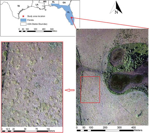
The proposed object-based classification approach was tested on a 677 m x 518 m area, which is part of a 31,000-acre ranch, located in Southern Florida, between Lake Okeechobee and the city of Arcadia. The ranch is composed of diverse tropical forage grass pastures, palmetto wet and dry prairies, pine flatwoods, and large interconnecting marsh of native grass wetlands (Grasslands). The study area is infested by Cogon Grass (Imperata cylindrica), as shown in the lower left corner of Figure 1. The land also hosts cabbage palm and live oak hammocks scattering along the lengths of copious creeks, gullies, and wetlands. All the classes, except the shadow class, were assigned according to the standard of vegetation classification for South Florida natural areas (Rutchey et al. 2006).

Figure 1. Study area: left corner highlight the area seriously impacted by invasive vegetation Cogon Grass.

The Cogan grass class is defined due to its harmful effect on the region as an invasive species. Cogon Grass is considered one of the top 10 worst invasive weeds in the world (Holm et al. 1977). The grass is not palatable as a livestock forage, decreases native plant biodiversity and wildlife habitat quality, increases fire hazard, and lowers the value of real estate. Several agencies, including United States Army Corps of Engineers (USACE) are involved in routine monitoring and control operations to limit the spread of Cogan grass in Florida. These efforts will greatly benefit from developing an efficient way to classify Cogan grass from UAS imagery. Our objective is to classify the Cogon Grass (species level) and five other community-level classes as well as the shadow class as listed in Table 1.

Table 1. Land cover classes in the study area.

Class ID	Class name	Description
CG	Cogon Grass	Cogon Grass (Imperata cylindrica) is an invasive, nonnative grass which occurs in Florida and several other Southeastern US states.
IP	Improved Pasture	A sown pasture that includes introduced pasture species, usually grasses in combination with legumes. These are generally more productive than the local native pastures, have higher protein and metabolizable energy and are typically more digestible. In our case, we also assume it is not infested by Cogon Grass.
SUs	Saw Palmetto Shrubland	Saw Palmetto (Serenoa repens) dominant shrubland.
MFB	Broadleaf Emergent Marsh	Broadleaf emergent dominated freshwater marsh. It can be found throughout Florida.
MFG	Graminoid Freshwater Marsh	Graminoid dominated freshwater marsh. It can be found throughout Florida.
FHp	Hardwood Hammock – Pine Forest	A co-dominate mix (40/60 to 60/40) of Slash Pine (Pinus elliottii var. densa) with Laural Oak (Quercus laurifolia), Live Oak (Q. virginiana), and/or Cabbage Palm (Sabal palmetto).
Shadow	Shadow	Shadow of all kinds of objects in the study area.

2.2. UAS image acquisition and preprocessing

The images used in this study were captured by the USACE-Jacksonville District using the NOVA 2.1 small UAS. A flight mission was designed with 83% forward overlap and 50% sidelap was planned and implemented. A Canon EOS REBEL SL1 digital camera is used in this study. The CCD sensor of this camera has 3456 x 5184 pixels. The images are synchronized with onboard navigation grade GPS receiver to provide image locations. Five ground control points were established (four near the four corners and one close to the center of the study area) and used in the photogrammetric solution. More details on the camera and flight mission parameters are listed in Table 2. During the UAS flight mission, sun zenith angle changed from 70° to 80°. The images are normalized to a common sun zenith angle of 75° using (Koukal and Atzberger 2012):

Table 2. Summary of sensor and flight procedure.

Items	Description
UAS type	Light UAS with Fixed wing
Sensor name	Canon EOS REBEL SL1
Sensor type	CCD
Pixel dimension	5184 x 3456
Length of focus	20mm
Sensor size	22.3 x 14.9 mm
Channels	RGB
Takeoff time	29/10/2015 16:54:51 EDT^a
Landing time	29/10/2015 17:49:33 EDT^a
Takeoff latitude	27.22736549
Takeoff longitude	−81.51152802
Average wind speed	5.1 m/s
Average altitude	302.7 m
Average pixel size	6.5 cm
Forward overlap	83%
Side overlap	50%
across-track
along-track

^aEastern Daylight Time.

^bField of view in degree.

where is the original UAS image i digital numbers and is the zenith angle of the sun when image i was taken.

2.3. Orthoimage creation and segmentation

The Agisoft Photoscan Pro version 1.2.4 software was used to implement the bundle block adjustment on a total of 1397 UAS images of the study area. The software was used to produce and export a three-band (red, green, and blue) 6 cm resolution orthoimage, a 27 cm digital surface model (DSM), and the camera exterior and interior orientation parameters. The three-band RGB orthoimage together with the DSM was analyzed using object-based analysis techniques. The Trimble’s eCognition software (Developer 2012) was used to segment the orthoimage image.

One of the most important options controlling the segmentation process is the scale parameter. Using small segmentation scale results in smaller and probably more homogeneous objects; however, very small object size brings the analysis closer to a pixel-based analysis. It increases the computational burden due to a large number of created objects and may affect the quality of the information extracted from each object (e.g. textual information). On the other hand, having large objects tends to produce mixed classes within the objects. Automatic selection of the best segmentation scale and/or the use of multi-resolution segmentation in the classification process is still an active research (Drăguţ et al. 2014) topic. However, in this research, we manually experimented with multiple segmentation scales as well as other parameters involved in the segmentation process and chose the scale (50), shape (0.2), and compactness (0.5) parameters (Developer 2012) that gave visually appealing segmentation results across the majority of the orthoimage. This process resulted in 40,239 objects within the study area.

Based on the segmented orthoimage, USACE ecologist responsible for managing this study area helped prepare a land cover reference map by inspecting the orthoimage to assign class labels to the orthoimage objects. For objects that could not be identified on the orthoimage, field visits were conducted. Based on this reference map, 1400 objects were randomly selected out of the total 40,239 objects to test (assess) the accuracy of the classification results. Within the remaining 38,839 objects, 700, 2100, and 3500 objects were randomly selected to generate three sets of training samples. All the classification experiments shared the same testing object samples for evaluating the classification performances and each classification method was implemented using the three training sample datasets, separately to investigate the sample size impact on classification accuracy.

3. Methods

3.1. Conventional OBIA classification using RF and SVM

The workflow of traditional object-based image classification, commonly applied to high-resolution orthoimages as implemented in the Trimble’s eCognition software (Developer 2012) can be summarized in three main steps: (1) Image segmentation into objects using a predefined set of parameters such as the segmentation scale and shape weight, (2) Extraction of features such as mean spectral band values and the standard deviation of the band values for each object in the segmented image, and (3) Train and implement a classifier such as the SVM (Scholkopf and Smola 2001), RF (Breiman 2001), or neural network (Yegnanarayana 2009) classifiers.

RF and SVM are selected as representatives of conventional classifiers due to their extensive adoptions and reliable performance for various remote sensing applications such as individual tree crown delineation (Liu, Im, and Quackenbush 2015), wet graminoid/sedge community mapping (Szantoi et al. 2013), forest aboveground biomass estimation (Ajaz Ahmed et al., 2017; Gleason and Im 2012; Li et al. 2014), convective cloud detection (Lee et al. 2017), drought forecasting and assessment (Park et al. 2016; Rhee and Im 2017), soil moisture monitoring(Im et al. 2016), etc. In this study, mean, standard deviation, maximum, and minimum values for red, green, and blue bands were extracted for classifications using RF and SVM. Gray-Level Co-Occurrence Matrix features were excluded from the features list for classification after it was tested and found unuseful to improve the classification accuracy. Geometric features including object boundary, object area, shape index, and boundary index as defined in eCognition (2012) were neither considered for classification in our study according to our preliminary test results and previous studies (Yu et al. 2006) showing they are not helpful for OBIA classification of natural land cover scenes.

The RF and SVM parameters were adjusted to make sure their performance as good as possible for our dataset. For example, different numbers of RF trees for RF were tested from 50 to 150 at 10 tree intervals. Classification accuracy did not change much as the number of the trees changed within this range. Three types of kernels (Gaussian, linear to polynomial kernels) for SMV were tested in our preliminary experiments with little impact on the resulting SVM classification accuracy. We adopted the one-versus-one option of the SVM classifier instead of the one-versus-all strategy based on previous studies (Hsu and Lin 2002). RF with 50 trees and SVM with Gaussian kernel were used to generate the classification results presented in this study. OBIA using SVM and RF are denoted SVM-OBIA and RF-OBIA, respectively. SVM-OBIA and RF-OBIA were both experimented with 700, 2100, and 3500 training samples. Adding the training sample size to the RF and SVM experiment names generated the SVM-OBIA-700, SVM-OBIA-2100, and SVM-OBIA-3500 notations for the SVM experiments and the RF-OBIA-700, RF-OBIA-2100, and RF-OBIA-3500 results for the RF experiments, respectively.

3.2. OBIA classification using DCNN

The input of DCNN is image patches, that is, rectangular subsets of the image. In our study, for each object resulting from the image segmentation process, an adaptive window exactly enclosing this object is extracted and used as an image patch representing the object. Following the notations introduced in last section to name the experiments, we denoted the DCNN experiments as DCNN-OBIA-700, DCNN-OBIA-2100, and DCNN-OBIA-3500 results.

The DCNN classifier used in this study is a 50-layer DCNN called deep residual nets introduced by He et al. (2016). In deep residual nets, instead of directly learning the underlying mapping, learning is performed to obtain the residual mapping . The desired underlying mapping is then obtained by , which forms the building block of deep residual nets. In our study, we used this building block to build a network of 50 layers, as implemented by MatConNet (Vedaldi and Lenc 2015). Only one fully connected layer is attached at the end of the network and the other layers belonged to the convolutional and other related layers such as the Rectified Linear Unit (ReLU) (Nair and Hinton 2010), normalization (Ioffe and Szegedy 2015), and pooling (Scherer, Müller, and Behnke 2010) layers.

3.3. OBIA classification using FCN

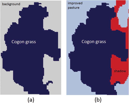
Similar to the DCNN-OBIA classifier, OBIA using FCN also requires image patches as input. Different from DCNN-OBIA, one complete training sample for FCN includes an image patch and a matrix of the same dimension as the image patch (in terms of the number of rows and columns), representing the label of each pixel of the image patch. There are two options for generating the labels of the image patch pixels based on how the pixels between the object boundary and image patch boundary are being labeled (Figure 2). In the first option (Option I), all the pixels surrounding the object are disregarded by labeling them simply as background, while for the second option (option II), each pixel is labeled with its class type.

Figure 2. Two options for generating training samples: (a) option I labels the surrounding pixels as background regardless of their actual class types and (b) option II labels all the pixels with their true labels.

Figure 2 illustrates the two methods for preparing the training samples used in this study. In Figure 2a, a Cogon Grass object is located at the center, representing the object under consideration. Pixels between this object boundary and image patch boundary are labeled as background regardless of their true labels. In Figure 2b, all the surrounding pixels are labeled with their class types, such as Improved Pasture and Shadow. Option I samples can be generated directly from existing training samples used by other classification methods (SVM-OBIA, RF-OBIA, and DCNN-OBIA), while option II samples require extra efforts to manually label the pixels surrounding the object. It is our hypothesis that option II samples would produce higher accuracy due to more information contained in the samples. OBIA classifications using FCN with option I and II samples are denoted as FCN-I-OBIA and FCN-II-OBIA, respectively. Following the previous notation convention for testing 700, 2100, and 3500 training samples, the FCN experiments are named: FCN-I-OBIA-700, FCN-I-OBIA-2100, FCN-I-OBIA-3500, FCN-II-OBIA-700, FCN-II-OBIA-2100, and FCN-II-OBIA-3500.

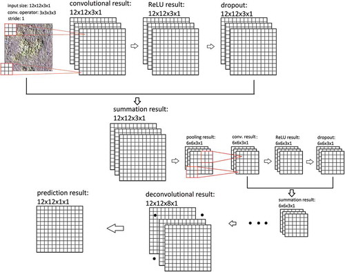
Figure 3 shows the structure of the FCN used in this study. For illustration purposes, we assume the input layer size has 12 x 12 as row by column numbers. The FCN and DCNN tested in this study have similar layer types, such as the summation operation (He et al. 2016), ReLU (Nair and Hinton 2010), dropout layer (Srivastava et al. 2014), and pooling (Scherer, Müller, and Behnke 2010) layers. They differ with each other in terms of structure, primarily because FCN requires the deconvolutional operation to make the final output layer having the same row and column numbers as the input layer size, as shown in Figure 3, and this critical operation enables the pixel-wise classification within the FCN image patch. The output of the last activation layer for FCN has the dimension “row*column* number of classes,” while for the DCNN it is just “number of classes.” We applied an object mask to the FCN output to find the majority pixel label within the object boundary and assigned this label to the patch (object) as its final FCN-OBIA classification result. To make better comparison of DCNN and FCN, we configured them to make them accept the same patch size (224 x 224). All image patches corresponding objects with different sizes are resized to 224 x 224 patches before they are input into DCNN and FCN.

Figure 3. Flow chart of conducted experiments.

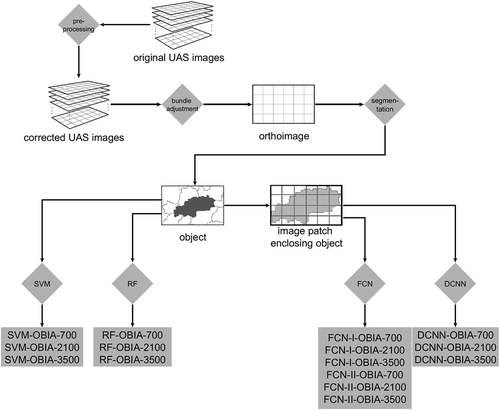
Figure 4 shows a simplified flowchart of the experiments conducted in this study. Bundle adjustment was applied to the UAS images to generate an orthoimage, which was then segmented to generate the objects. Based on these objects, either features were extracted for the SVM and RF classifiers, or image patches were extracted for the DCNN and FCN classifiers. For the FCN experiment, two types of training samples illustrated in Figure 2 generated two sets of classification results (FCN-I-OBIA and FCN-II-OBIA). The whole procedure generated 15 experiment results.

Figure 4. Flow chart of conducted experiments.

4. Results and discussion

Figure 5 shows the overall accuracies of the 15 classification experiments shown in Figure 4. When 700 training samples were used, RF-OBIA and SVM-OBIA obtained 58.9% and 62.4% overall accuracy, respectively, and both were higher than the 51.8% overall accuracy resulting from DCNN-OBIA, but lower than the 69.2% and 77.0% achieved by FCN-I-OBIA and FCN-II-OBIA, respectively. As the size of training samples becomes 2100, DCNN-OBIA accuracy increased significantly to 67.6%, overtaking the RF-OBIA and SVM-OBIA, which had 62.8% and 66.1%, respectively. Even though DCNN-OBIA still produced lower accuracy than FCN-I-OBIA and FCN-II-OBIA at this point, its difference with FCN-I-OBIA decreased from 17.4% using 700 training samples to 6.1% with 2100 training samples. As the training sample size grows to 3500, the DCNN-OBIA improved and slightly exceeded FCN-I-OBIA (76.9% vs. 76.3%). While both RF-OBIA and SVM-OBIA also continued to show higher accuracy as the training sample size increased from 2100 to 3500, the accuracy improvements for these two conventional classifiers were much less impressive than that of the DCNN (improvement is 2.8% for RF-OBIA, 1.5% for SVM-OBIA vs. 9.3% for DCNN-OBIA when training sample size increased from 2100 to 3500). FCN always gave much better performance than all other classifiers regardless of the number of training samples or the training sample preparation method (GCN-I-OBIA or FCN-II-OBIA). The advantages of FCN over traditional classifiers such as RF is reported in previous studies such as the study by Piramanayagam et al. (2016), who applied FCN using orthophoto and DSM, obtaining 88% accuracy, higher than the 86.3% accuracy, achieved by RF.

Figure 5. Overall accuracies obtained from five classification methods with three sets of training samples.

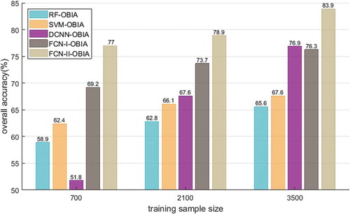
SVM consistently showed slightly better performance than RF regardless of training sample size. This observation is opposite to the study by Liu et al. (2013), which showed RF giving much better accuracy than SVM, but consistent with other studies that showed SVM performing better than (Statnikov, Wang, and Aliferis 2008) or similar to (Díaz-Uriarte and De Andres 2006; Pal 2005) RF. The accuracies presented by the conventional classifiers in this study were comparable with other studies that mapped wetland land cover types in South Florida using UAS images(Pande-Chhetri et al. 2017; Zweig et al. 2015).

The observation that DCNN only obtained slightly better accuracy than SVM when training sample size is 2100 is in line with the results from Hu et al. (2015), that showed accuracy improvements of 0.94%, 2.56%, and 2.04% for three datasets, respectively, by DCNN compared with SVM results using pixel-based classification. However, based on the result from Figure 5, the advantage of DCNN over SVM in terms of overall accuracy is expected to become more obvious when massive training samples are available, with advantage of DCNN over SVM ranging from negative 10.6% at sample size 700 to positive 9.3% at sample size 3500. The behaviors of DCNN shown in Figure 5 is consistent with the generally claimed but rarely verified notion in remote sensing community that deep learning networks require massive training samples to trigger its power (Cheng, Zhou, and Han 2016; Xie et al. 2015; Zhao and Du 2016). In this study, 3500 training samples are already enough for DCNN to produce much better performance than conventional classifiers. This result stresses the importance of the role played by the training sample size in comparing DCNN with conventional classifiers.

FCN seems most efficient to utilize the training samples, especially when sample size is not large, with FCN-I-OBIA always showing better accuracy compared to DCNN-OBIA as shown in Figure 5. The gap between DCNN-OBIA and FCN-I-OBIA classification accuracy becomes smaller as the sample size increases. Sherrah (2016) compared patch-based DCNN and FCN and found FCN outperforming patch-based DCNN with 87.17% to 83.46% overall accuracy. Figure 5 reveals that the advantages of FCN over DCNN can be strongly dependent on training sample size. It should be mentioned here that the samples prepared for DCNN can be directly converted to samples for FCN-I-DCNN (see Figure 2a) without any extra effort in sample preparation, which gives a great advantage to FCN implementation over DCNN, especially in the case of small sample size. Adding more label information to the training sample object (see Figure 2b) enabled the implementation of the FCN-II-OBIA, which according to the Figure 5, always showed the highest accuracy for all three sample sizes. This indicates that using label information of the pixels surrounding the object in each patch is very useful for FCN to improve the classification, and highlights the advantage of FCN over DCNN in terms of its ability to learn from such formation.

It is generally believed that deep learning networks require massive training data due to their large number of parameters that need to be learnt. This is consistent with the behavior of DCNN observed in this study, which has 25,610,152 parameters in total and required considerable number of training samples (e.g. 3500 samples) to perform better than conventional classifiers. However, the belief that deep learning networks with having more parameters requires more training samples to show better deep learning performance may not be true all the time. For example, the FCN used in this study has 134,382,239 parameters (much larger than the 25,610,152 DCNN parameters) with the same number of training samples and label information (DCNN-OBIA versus FCN-I-OBIA); however, the classification accuracy of the FCN was not only higher than conventional classifiers, but also higher than the DCNN when smaller number of training samples were used.

While DCNN and FCN in this study have similar layer types, FCN has the exclusive deconvolutional layer to allow it to perform the training end-to-end and pixel-to-pixel, instead of on the image patch level as is the case for DCNN. We think having accurate label information might be one of the important reasons that FCN-I-OBIA outperformed the DCNN-OBIA when both methods utilized the same small number of training samples. The importance of having accurate and rich label information is also demonstrated when comparing the FCN-I-OBIA and FCN-II-OBIA results. These two methods use exactly the same FCN and just because FCN-II-OIBA training samples have exact pixel labels for the whole patch, it always performed much better than FCN-I-OBIA when the same number of training samples is used. As the training dataset size became larger, DCNN-OBIA and FCN-I-OBIA tend to accumulate high number of label information, and this may explain why the gap between DCNN-OBIA and FCN-I-OBIA classification results is reduced when the number of training samples increased. Even though the number of parameters and structures are different between FCN and DCNN, it seems that one of the primary factor determining their performances is the number and richness of label information in the training samples. However, more studies were required to verify this conjecture, since DCNN and FCN used in this study were different from each other not only because FCN has the convolutional layer, which is missing in DCNN, but also because their parameter numbers, detailed structure, and layer types are neither exactly the same.

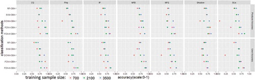
Figure 6 shows the producer and user accuracies for seven class types obtained using five OBIA classification methods experimented with three sets of training samples separately. Regardless of which classification method was used, increasing the sample size always improved the producer and user accuracy for almost all the classes, with only few exceptions. FCN-II-OBIA consistently showed highest accuracy across all the classes with very few exceptions (e.g., when sample size is 2100, FCN-I-OBIA gave slightly better user accuracy than FCN-II-OBIA for SUs).

Figure 6. Producer and user accuracies for different classification methods with different sets of training samples.

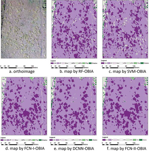
Figure 7 shows the maps generated by five classification approaches using 3500 training samples. The first row shows the map by conventional classifiers and the second row presents the maps produced using deep learning networks. To our best knowledge, Figure 7d and f are the first published maps that were generated using object-based method with FCN being the classifier. Figure 7e is the first published map for natural environment that was created with object-based method using DCNN. Figure 8 is the zoom-in version of bottom left part of Figure 7 focusing on Cogon grass area. A visual inspection of Figures 7 and 8 indicates that deep learning networks can produce more appealing maps than conventional classifiers, as is consistent with their high overall accuracies (Figure 5).

Figure 7. Maps generated by five classification methods using 3500 training samples.

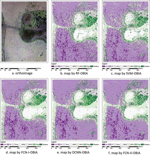
Figure 8. Zoom-in version of maps focusing on Cogon grass area.

The maps in Figure 7 shows that conventional classifiers mislabel the IP as MFG classes more often than other class types. The MFG represents marsh land cover, one of the typical land covers in South Florida wetlands (Arthington et al. 2007; Swain et al. 2013). IP is relatively flat and some areas are low lying and tend to flood frequently, which may make the IP and MFG spectrally similar. It should be noted that UAS images used in this study contains only RGB bands using low-cost off-the-shelf camera. The use of hyperspectral sensor onboard UAS (Pajares 2015; Saito et al. 2014; Zarco-Tejada, González-Dugo, and Berni 2012) has been increased recently due to the increase in UAS payload and navigation sensors affordability. Using hyperspectral imagery should facilitate accurate classification of spectrally similar land covers.

Table 3 shows the confusion matrix of the FCN-II-OBIA-3500 classification. The table shows FCN-II-OBIA produced high Cogan Grass classification accuracy with 95.0% and 89.2% producer and user accuracy, respectively. Further examination of Table 3 indicates Shadow class is the primary error source among all the classes with the lowest producer accuracy (74.1%). The Shadow class row in Table 3 shows all other classes having a certain number of objects ranging from 1 to 10 mistakenly classified as Shadow. Furthermore, a large number of SUs objects were mislabeled as Shadow, decreasing the producer accuracy of the SUs class substantially. Figure 7 shows that the SUs class is dominated by Saw Palmetto, which usually surrounds the MFB, the Broadleaf Emergent arsh, and is scattered with higher hardwood from the FHp class. FHp class constituents can cast Shadow onto SUs, making the class Shadow easily confused with SUs. Such a confusion between the Shadow class and the rest classes maybe attributed to the fact that Shadow object can be viewed as a layer overlaid on other class surfaces. The transparency of this layer depends on the vegetation cover causing the shadow as well as illumination and viewing geometry.

Table 3. Confusion matrix for FCN-II-OBIA classification results.

	CG	IP	SUs	MFB	MFG	FHp	Shadow	Producer accuracy
CG	190	9	0	0	1	0	0	95.0
IP	15	164	3	0	11	2	5	82.0
SUs	3	0	151	0	3	18	25	75.5
MFB	1	0	0	176	17	0	6	88.0
MFG	2	6	10	14	149	7	12	74.5
FHp	1	0	10	0	2	176	11	88.0
Shadow	1	10	8	0	2	10	169	84.5
User accuracy	89.2	86.8	83.0	92.6	80.5	82.6	74.1	83.9

5. Conclusion

This study analyzed the use of conventional and deep learning classification techniques under the OBIA framework in classifying wetland land cover in South Florida. The study compared the performance of the DCNN and FCN deep learning classifiers. Furthermore, the study tested the use of two types of FCN sample preparation methods to examine whether including object surrounding information would improve the performance of the FCN classification.

The results indicate that the number of training samples played an important role in determining the performance of DCNN when compared with conventional classifiers. DCNN may not necessarily perform better than conventional classifiers when a relatively small training set size is used; however, its advantages over conventional classifiers would easily show up if trained with a large size of training samples. FCN is more efficient in utilizing the information in the training dataset than DCNN with its ability to perform pixel-based training, resulting in better classification performances. However, if a large number of training samples are used, FCN and DCNN tend to show similar performances when both only use object label information. Adding object surrounding label information to the training samples is very useful for FCN to improve its classification performance, consistently producing the highest classification accuracy regardless of the training sample size.

This study shows that deep learning networks is recommended for processing very high resolution images collected by UAS for mapping wetland covers using OBIA, provided that a large volume of training samples are available. FCN rather than DCNN is suggested for OBIA if a relatively low number of training samples are available. Having surrounding pixel labeled for training samples is always suggested if higher accuracy is desired. For future studies, we suggest using the multi-view data extracted from the UAS to investigate whether those multi-view data can trigger the power of the deep learning networks without massive training samples.

Disclosure statement

No potential conflict of interest was reported by the authors.

References

- Ajaz Ahmed, M. A., A. Abd-Elrahman, F. J. Escobedo, W. P. Cropper Jr, T. A. Martin, and N. Timilsina. 2017. “Spatially-Explicit Modeling of Multi-Scale Drivers of Aboveground Forest Biomass and Water Yield in Watersheds of the Southeastern United States.” 199: 158.
- Alshehhi, R., P. R. Marpu, W. L. Woon, and M. Dalla Mura. 2017. “Simultaneous Extraction of Roads and Buildings in Remote Sensing Imagery with Convolutional Neural Networks.” ISPRS Journal of Photogrammetry and Remote Sensing 130: 139–149. doi:10.1016/j.isprsjprs.2017.05.002.
- Ahmed, Mukhtar Ahmed Ajaz, et al. “Spatially-explicit modelingof multi-scale drivers of aboveground forest biomass and water yield in watersheds of the Southeastern United States”. Journal of Environmental Management 199 (2017): 158–171.
- Arthington, J., F. Roka, J. Mullahey, S. Coleman, R. Muchovej, L. Lollis, and D. Hitchcock. 2007. “Integrating Ranch Forage Production, Cattle Performance, and Economics in Ranch Management Systems for Southern Florida.” Rangeland Ecology & Management 60: 12–18. doi:10.2111/05-074R1.1.
- Belgiu, M., and L. Drăguţ. 2016. “Random Forest in Remote Sensing: A Review of Applications and Future Directions.” ISPRS Journal of Photogrammetry and Remote Sensing 114: 24–31. doi:10.1016/j.isprsjprs.2016.01.011.
- Blaschke, T. 2010. “Object Based Image Analysis for Remote Sensing.” ISPRS Journal of Photogrammetry and Remote Sensing 65: 2–16. doi:10.1016/j.isprsjprs.2009.06.004.
- Breiman, L. 2001. “Random Forests.” Machine Learning 45: 5-32. doi:10.1023/A:1010933404324.
- Camacho-de Coca, F., F. M. Bréon, M. Leroy, and F. J. Garcia-Haro. 2004. “Airborne Measurement of Hot Spot Reflectance Signatures.” Remote Sensing of Environment 90: 63–75. doi:10.1016/j.rse.2003.11.019.
- Cheng, G., P. Zhou, and J. Han. 2016. “Learning Rotation-Invariant Convolutional Neural Networks for Object Detection in VHR Optical Remote Sensing Images.” IEEE Transactions on Geoscience and Remote Sensing 54: 7405–7415. doi:10.1109/TGRS.2016.2601622.
- Cortes, C., and V. Vapnik. 1995. “Support-Vector Networks.” Machine Learning 20: 273–297. doi:10.1007/BF00994018.
- Davis, S., and J. C. Ogden. 1994. Everglades: The Ecosystem and Its Restoration. CRC Press, Florida, Boca Raton.
- Developer, E. 2012. Trimble eCognition Developer 8.7 Reference Book. Trimble Germany GmbH, Munich.
- Díaz-Uriarte, R., and S. A. De Andres. 2006. “Gene Selection and Classification of Microarray Data Using Random Forest.” BMC Bioinformatics 7: 3. doi:10.1186/1471-2105-7-3.
- Drăguţ, L., O. Csillik, C. Eisank, and D. Tiede. 2014. “Automated Parameterisation for Multi-Scale Image Segmentation on Multiple Layers.” ISPRS Journal of Photogrammetry and Remote Sensing 88: 119–127. doi:10.1016/j.isprsjprs.2013.11.018.
- eCognition, 2012. Features Reference, http://community.ecognition.com/home/features-reference.
- Fernández, T., J. L. Pérez, J. Cardenal, J. M. Gómez, C. Colomo, and J. Delgado. 2016. “Analysis of Landslide Evolution Affecting Olive Groves Using UAV and Photogrammetric Techniques.” Remote Sensing 8: 837. doi:10.3390/rs8100837.
- Ferriter, A., K. Serbesoff-King, M. Bodle, C. Goodyear, B. Doren, and K. Langeland. 2004. “Exotic Species in the Everglades Protection Area.” In: 2004 Everglades Consolidated Report, 11–15. South FloridaWater Management District (SFWMD) and Florida Department ofEnvironmental Protection (FDEP).
- Gleason, C. J., and J. Im. 2012. “Forest Biomass Estimation from Airborne LiDAR Data Using Machine Learning Approaches.” Remote Sensing of Environment 125: 80–91. doi:10.1016/j.rse.2012.07.006.
- Grybas, H., L. Melendy, and R. G. Congalton. 2017. “A Comparison of Unsupervised Segmentation Parameter Optimization Approaches Using Moderate- and High-Resolution Imagery.” GIScience & Remote Sensing,54: 1–19.
- He, K., X. Zhang, S. Ren, and J. Sun. 2016. “Deep Residual Learning for Image Recognition.” In: Proceedings of the IEEE Conference on Computer Vision and Pattern Recognition, IEEE, 770–778.
- Hinton, G., L. Deng, D. Yu, G. E. Dahl, A.-R. Mohamed, N. Jaitly, A. Senior, V. Vanhoucke, P. Nguyen, and T. N. Sainath. 2012. “Deep Neural Networks for Acoustic Modeling in Speech Recognition: The Shared Views of Four Research Groups.” IEEE Signal Processing Magazine 29: 82–97. doi:10.1109/MSP.2012.2205597.
- Hinton, G. E., S. Osindero, and Y.-W. Teh. 2006. “A Fast Learning Algorithm for Deep Belief Nets.” Neural Computation 18: 1527–1554. doi:10.1162/neco.2006.18.7.1527.
- Holm, L. G., D. L. Plucknett, J. V. Pancho, and J. P. Herberger. 1977. The World’s Worst Weeds. University Press, Honolulu, Hawaii.
- Hsu, C.-W., and C.-J. Lin. 2002. “A Comparison of Methods for Multiclass Support Vector Machines.” IEEE Transactions on Neural Networks 13: 415–425. doi:10.1109/72.991427.
- Huval, B., T. Wang, S. Tandon, J. Kiske, W. Song, J. Pazhayampallil, M. Andriluka, P. Rajpurkar, T. Migimatsu, and R. Cheng-Yue. 2015. “An Empirical Evaluation of Deep Learning on Highway Driving.” arXiv Preprint arXiv:1504.01716.
- Hu, W., Huang, Y., Wei, L., Zhang, F., Li, H., 2015. Deepconvolutional neural networks for hyperspectral image classification. Journal of Sensors.
- Im, J., J. Jensen, and J. Tullis. 2008. “Object‐Based Change Detection Using Correlation Image Analysis and Image Segmentation.” International Journal of Remote Sensing 29: 399–423. doi:10.1080/01431160601075582.
- Im, J., S. Park, J. Rhee, J. Baik, and M. Choi. 2016. “Downscaling of AMSR-E Soil Moisture with MODIS Products Using Machine Learning Approaches.” Environmental Earth Sciences 75: 1120. doi:10.1007/s12665-016-5917-6.
- Ioffe, S., and C. Szegedy. 2015. “Batch Normalization: Accelerating Deep Network Training by Reducing Internal Covariate Shift.” arXiv Preprint arXiv:1502.03167.
- Jensen, J. R., K. Rutchey, M. S. Koch, and S. Narumalani. 1995. “Inland Wetland Change Detection in the Everglades Water Conservation Area 2A Using a Time Series of Normalized Remotely Sensed Data.” Photogrammetric Engineering and Remote Sensing 61: 199–209.
- Ke, Y., L. J. Quackenbush, and J. Im. 2010. “Synergistic Use of QuickBird Multispectral Imagery and LIDAR Data for Object-Based Forest Species Classification.” Remote Sensing of Environment 114: 1141–1154. doi:10.1016/j.rse.2010.01.002.
- Keddy, P. A. 2010. Wetland Ecology: Principles and Conservation. Cambridge University Press: NY, New York City.
- Koukal, T., and C. Atzberger. 2012. “Potential of Multi-Angular Data Derived from a Digital Aerial Frame Camera for Forest Classification.” IEEE Journal of Selected Topics in Applied Earth Observations and Remote Sensing 5: 30–43. doi:10.1109/JSTARS.2012.2184527.
- Krizhevsky, A., I. Sutskever, and G. E. Hinton. 2012. “Imagenet Classification with Deep Convolutional Neural Networks.” Advances in Neural Information Processing Systems 1097–1105.
- Kussul, N., M. Lavreniuk, S. Skakun, and A. Shelestov. 2017. “Deep Learning Classification of Land Cover and Crop Types Using Remote Sensing Data.” IEEE Geoscience and Remote Sensing Letters 14: 778–782. doi:10.1109/LGRS.2017.2681128.
- LeCun, Y., Y. Bengio, and G. Hinton. 2015. “Deep Learning.” Nature 521: 436–444. doi:10.1038/nature14539.
- Lee, S., H. Han, J. Im, E. Jang, and M.-I. Lee. 2017. “Detection of Deterministic and Probabilistic Convection Initiation Using Himawari-8 Advanced Himawari Imager Data.” Atmospheric Measurement Techniques 10: 1859–1874. doi:10.5194/amt-10-1859-2017.
- Li, L., Y. Chen, T. Xu, R. Liu, K. Shi, and C. Huang. 2015. “Super-Resolution Mapping of Wetland Inundation from Remote Sensing Imagery Based on Integration of Back-Propagation Neural Network and Genetic Algorithm.” Remote Sensing of Environment 164: 142–154. doi:10.1016/j.rse.2015.04.009.
- Li, M., J. Im, L. J. Quackenbush, and T. Liu. 2014. “Forest Biomass and Carbon Stock Quantification Using Airborne LiDAR Data: A Case Study over Huntington Wildlife Forest in the Adirondack Park.” IEEE Journal of Selected Topics in Applied Earth Observations and Remote Sensing 7: 3143–3156. doi:10.1109/JSTARS.2014.2304642.
- Li, M., L. Ma, T. Blaschke, L. Cheng, and D. Tiede. 2016a. “A Systematic Comparison of Different Object-Based Classification Techniques Using High Spatial Resolution Imagery in Agricultural Environments.” International Journal of Applied Earth Observation and Geoinformation 49: 87–98. doi:10.1016/j.jag.2016.01.011.
- Li, Z., W. Shi, P. Lu, L. Yan, Q. Wang, and Z. Miao. 2016b. “Landslide Mapping from Aerial Photographs Using Change Detection-Based Markov Random Field.” Remote Sensing of Environment 187: 76–90. doi:10.1016/j.rse.2016.10.008.
- Liu, M., Wang, M., Wang, J., Li, D., 2013. Comparison of random forest, support vector machine and back propagation neural network for electronic tongue data classification: Application to the Page 2 of 4 recognition of orange beverage and Chinese vinegar. Sensors and Actuators B: Chemical 177, 970–980.
- Liu, T., J. Im, and L. J. Quackenbush. 2015. “A Novel Transferable Individual Tree Crown Delineation Model Based on Fishing Net Dragging and Boundary Classification.” ISPRS Journal of Photogrammetry and Remote Sensing 110: 34–47. doi:10.1016/j.isprsjprs.2015.10.002.
- Long, J., E. Shelhamer, and T. Darrell. 2015. “Fully Convolutional Networks for Semantic Segmentation.” In: Proceedings of the IEEE Conference on Computer Vision and Pattern Recognition, IEEE, 3431–3440.
- Lu, B., and Y. He. 2017. “Species Classification Using Unmanned Aerial Vehicle (UAV)-Acquired High Spatial Resolution Imagery in a Heterogeneous Grassland.” ISPRS Journal of Photogrammetry and Remote Sensing 128: 73–85. doi:10.1016/j.isprsjprs.2017.03.011.
- Ma, L., M. Li, X. Ma, L. Cheng, P. Du, and Y. Liu. 2017. “A Review of Supervised Object-Based Land-Cover Image Classification.” ISPRS Journal of Photogrammetry and Remote Sensing 130: 277–293. doi:10.1016/j.isprsjprs.2017.06.001.
- Ma, X., H. Wang, and J. Wang. 2016. “Semisupervised Classification for Hyperspectral Image Based on Multi-Decision Labeling and Deep Feature Learning.” ISPRS Journal of Photogrammetry and Remote Sensing 120: 99–107. doi:10.1016/j.isprsjprs.2016.09.001.
- Makantasis, K., K. Karantzalos, A. Doulamis, and N. Doulamis. 2015. “Deep Supervised Learning for Hyperspectral Data Classification through Convolutional Neural Networks.” In: Geoscience and Remote Sensing Symposium (IGARSS), 2015 IEEE International, 4959–4962. IEEE.
- Marmanis, D., K. Schindler, J.D. Wegner, S. Galliani, and M Datcu.,Stilla, U., 2016. Classification with an edge: improving semanticimage segmentation with boundary detection. arXiv preprintarXiv: 1612.01337.
- Martínez-López, J., M. F. Carreño, J. A. Palazón-Ferrando, J. Martínez-Fernández, and M. A. Esteve. 2014. “Remote Sensing of Plant Communities as a Tool for Assessing the Condition of Semiarid Mediterranean Saline Wetlands in Agricultural Catchments.” International Journal of Applied Earth Observation and Geoinformation 26: 193–204. doi:10.1016/j.jag.2013.07.005.
- McGwire, K. C., M. A. Weltz, J. A. Finzel, C. E. Morris, L. F. Fenstermaker, and D. S. McGraw. 2013. “Multiscale Assessment of Green Leaf Cover in a Semi-Arid Rangeland with a Small Unmanned Aerial Vehicle.” International Journal of Remote Sensing 34: 1615–1632. doi:10.1080/01431161.2012.723836.
- Mitsch, W. J., and J. G. Gosselink. 2015. Wetlands. 5th ed. Hoboken, NJ: Wiley.
- Murakami, T., M. Yui, and K. Amaha. 2012. “Canopy Height Measurement by Photogrammetric Analysis of Aerial Images: Application to Buckwheat (Fagopyrum Esculentum Moench) Lodging Evaluation.” Computers and Electronics in Agriculture 89: 70–75. doi:10.1016/j.compag.2012.08.003.
- Nair, V., and G. E. Hinton. 2010. “Rectified Linear Units Improve Restricted Boltzmann Machines.” In: Proceedings of the 27th International Conference on Machine Learning (ICML-10), 807–814.
- Pajares, G. 2015. “Overview and Current Status of Remote Sensing Applications Based on Unmanned Aerial Vehicles (UAVs).” Photogrammetric Engineering & Remote Sensing 81: 281–330. doi:10.14358/PERS.81.4.281.
- Pal, M. 2005. “Random Forest Classifier for Remote Sensing Classification.” International Journal of Remote Sensing 26: 217–222. doi:10.1080/01431160412331269698.
- Pande-Chhetri, R., A. Abd-Elrahman, T. Liu, J. Morton, and V. L. Wilhelm. 2017. “Object-Based Classification of Wetland Vegetation Using Very High-Resolution Unmanned Air System Imagery.” European Journal of Remote Sensing 50: 564–576. doi:10.1080/22797254.2017.1373602.
- Park, S., J. Im, E. Jang, and J. Rhee. 2016. “Drought Assessment and Monitoring through Blending of Multi-Sensor Indices Using Machine Learning Approaches for Different Climate Regions.” Agricultural and Forest Meteorology 216: 157–169. doi:10.1016/j.agrformet.2015.10.011.
- Pastor, E., C. Barrado, P. Royo, E. Santamaria, J. Lopez, and E. Salami. 2011. “Architecture for a Helicopter-Based Unmanned Aerial Systems Wildfire Surveillance System.” Geocarto International 26: 113–131. doi:10.1080/10106049.2010.531769.
- Peppa, M., J. Mills, P. Moore, P. Miller, and J. Chambers. 2016. “Accuracy Assessment of a UAV-Based Landslide Monitoring System. ISPRS-International Archives of the Photogrammetry.” Remote Sensing and Spatial Information Sciences 895–902.
- Primicerio, J., S. F. Di Gennaro, E. Fiorillo, L. Genesio, E. Lugato, A. Matese, and F. P. Vaccari. 2012. “A Flexible Unmanned Aerial Vehicle for Precision Agriculture.” Precision Agriculture 13: 517–523. doi:10.1007/s11119-012-9257-6.
- Piramanayagam, S., Schwartzkopf, W., Koehler, F., Saber E., 2016. Classification of remote sensed images using random forests and deep learning framework, SPIE Remote Sensing. International Society for Optics and Photonics, pp. 100040L-100040L-100048.
- Rango, A., A. Laliberte, C. Steele, J. E. Herrick, B. Bestelmeyer, T. Schmugge, A. Roanhorse, and V. Jenkins. 2006. “Using Unmanned Aerial Vehicles for Rangelands: Current Applications and Future Potentials.” Environmental Practice 8: 159–168. doi:10.1017/S1466046606060224.
- Rhee, J., and J. Im. 2017. “Meteorological Drought Forecasting for Ungauged Areas Based on Machine Learning: Using Long-Range Climate Forecast and Remote Sensing Data.” Agricultural and Forest Meteorology 237: 105–122. doi:10.1016/j.agrformet.2017.02.011.
- Rutchey, K., T. Schall, R. Doren, A. Atkinson, M. Ross, D. Jones, M. Madden, L. Vilchek, K. Bradley, and J. Snyder. 2006. Vegetation Classification for South Florida Natural Areas. Petersburg, FL: US Geological Survey St.
- Saito, G., H. Seki, K. Uto, Y. Kosugi, and T. Komatsu. 2014. “Development of Hyperspectral Imaging Sensor, Which Mounted on UAV for Environmental Study at Coastal Zone.” In: 35th Asian Conference on Remote Sensing.
- Samseemoung, G., P. Soni, H. P. Jayasuriya, and V. M. Salokhe. 2012. “Application of Low Altitude Remote Sensing (LARS) Platform for Monitoring Crop Growth and Weed Infestation in a Soybean Plantation.” Precision Agriculture 13: 611–627. doi:10.1007/s11119-012-9271-8.
- Scherer, D., A. Müller, and S. Behnke. 2010. “Evaluation of Pooling Operations in Convolutional Architectures for Object Recognition.” Artificial Neural Networks–ICANN 2010: 92–101.
- Scholkopf, B., and A.J Smola., 2001. Learning with kernels: supportvector machines, regularization, optimization, and beyond. MIT press.
- Sheikh, P. A. 2002. “Florida Everglades Restoration: Background on Implementation and Early Lessons.” In: The Libraryof Congress: Congressional Research Service.
- Sherrah, J. 2016. “Fully Convolutional Networks For Densesemantic Labelling Of High-resolution Aerial Imagery.” Arxiv Preprint arxiv 1606: 02585.
- Silver, D., A. Huang, C. J. Maddison, A. Guez, L. Sifre, G. Van Den Driessche, J. Schrittwieser, I. Antonoglou, V. Panneershelvam, and M. Lanctot. 2016. “Mastering the Game of Go with Deep Neural Networks and Tree Search.” Nature 529: 484–489. doi:10.1038/nature16961.
- Simonyan, K., and A. Zisserman. 2014. “Very Deep Convolutional Networks for Large-Scale Image Recognition.” arXiv Preprint arXiv:1409.1556.
- Skeele, R. C., and G. A. Hollinger. 2016. Aerial Vehicle Path Planning for Monitoring Wildfire Frontiers, Field and Service Robotics, 455–467. Springer.
- Srivastava, N., G. E. Hinton, A. Krizhevsky, I. Sutskever, and R. Salakhutdinov. 2014. “Dropout: A Simple Way to Prevent Neural Networks from Overfitting.” Journal of Machine Learning Research 15: 1929–1958.
- Statnikov, A., L. Wang, and C. F. Aliferis. 2008. “A Comprehensive Comparison of Random Forests and Support Vector Machines for Microarray-Based Cancer Classification.” BMC Bioinformatics 9: 319. doi:10.1186/1471-2105-9-319.
- Suk, H.-I., S.-W. Lee, D. Shen, and A. S. D. N. Initiative. 2014. “Hierarchical Feature Representation and Multimodal Fusion with Deep Learning for AD/MCI Diagnosis.” NeuroImage 101: 569–582. doi:10.1016/j.neuroimage.2014.06.077.
- Suzuki, T., Y. Amano, T. Hashizume, S. Suzuki, and A. Yamaba. 2010. “Generation of Large Mosaic Images for Vegetation Monitoring Using a Small Unmanned Aerial Vehicle.” Journal of Robotics and Mechatronics 22: 212–220. doi:10.20965/jrm.2010.p0212.
- Swain, H. M., E. H. Boughton, P. J. Bohlen, and L. O. G. Lollis. 2013. “Trade-Offs among Ecosystem Services and Disservices on a Florida Ranch.” Rangelands 35: 75–87. doi:10.2111/RANGELANDS-D-13-00053.1.
- Szantoi, Z., F. Escobedo, A. Abd-Elrahman, S. Smith, and L. Pearlstine. 2013. “Analyzing Fine-Scale Wetland Composition Using High Resolution Imagery and Texture Features.” International Journal of Applied Earth Observation and Geoinformation 23: 204–212. doi:10.1016/j.jag.2013.01.003.
- Vedaldi, A., and K. Lenc. 2015. “Matconvnet: Convolutional Neural Networks for Matlab.” In: Proceedings of the 23rd ACM International Conference on Multimedia, 689–692. ACM.
- Vetrivel, A., M. Gerke, N. Kerle, F. Nex, and G. Vosselman. 2017. “Disaster Damage Detection through Synergistic Use of Deep Learning and 3D Point Cloud Features Derived from Very High Resolution Oblique Aerial Images, and Multiple-Kernel-Learning.” ISPRS Journal of Photogrammetry and Remote Sensing. doi:10.1016/j.isprsjprs.2017.03.001.
- Wang, C., R. T. Pavlowsky, Q. Huang, and C. Chang. 2016. “Channel Bar Feature Extraction for a Mining-Contaminated River Using High-Spatial Multispectral Remote-Sensing Imagery.” GIScience & Remote Sensing 53: 283–302. doi:10.1080/15481603.2016.1148229.
- Wright, C., and A. Gallant. 2007. “Improved Wetland Remote Sensing in Yellowstone National Park Using Classification Trees to Combine TM Imagery and Ancillary Environmental Data.” Remote Sensing of Environment 107: 582–605. doi:10.1016/j.rse.2006.10.019.
- Xie, M., N. Jean, M. Burke, D. Lobell, and S. Ermon. 2015. “Transfer Learning from Deep Features for Remote Sensing and Poverty Mapping.” arXiv Preprint arXiv:1510.00098.
- Yegnanarayana, B., 2009. Artificial neural networks. PHI Learning Pvt. Ltd
- Yu, Q., P. Gong, N. Clinton, G. Biging, M. Kelly, and D. Schirokauer. 2006. “Object-Based Detailed Vegetation Classification with Airborne High Spatial Resolution Remote Sensing Imagery.” Photogrammetric Engineering & Remote Sensing 72: 799–811. doi:10.14358/PERS.72.7.799.
- Yue, J., T. Lei, C. Li, and J. Zhu. 2012. “The Application of Unmanned Aerial Vehicle Remote Sensing in Quickly Monitoring Crop Pests.” Intelligent Automation & Soft Computing 18: 1043–1052. doi:10.1080/10798587.2008.10643309.
- Yunxia, H., L. Minzan, Z. Xijie, J. Liangliang, C. Xingping, and Z. Fusuo. 2005. “Precision Management of Winter Wheat Based on Aerial Images and Hyperspectral Data Obtained by Unmanned Aircraft.” In: Geoscience and Remote Sensing Symposium, 2005. IGARSS’05. Proceedings. 2005 IEEE International, 3109–3112. IEEE.
- Zarco-Tejada, P. J., V. González-Dugo, and J. A. Berni. 2012. “Fluorescence, Temperature and Narrow-Band Indices Acquired from a UAV Platform for Water Stress Detection Using a Micro-Hyperspectral Imager and a Thermal Camera.” Remote Sensing of Environment 117: 322–337. doi:10.1016/j.rse.2011.10.007.
- Zedler, J. B., and S. Kercher. 2004. “Causes and Consequences of Invasive Plants in Wetlands: Opportunities, Opportunists, and Outcomes.” Critical Reviews in Plant Sciences 23: 431–452. doi:10.1080/07352680490514673.
- Zedler, J. B., and S. Kercher. 2005. “Wetland Resources: Status, Trends, Ecosystem Services, and Restorability.” Annu. Rev. Environ. Resour. 30: 39–74. doi:10.1146/annurev.energy.30.050504.144248.
- Zeggada, A., F. Melgani, and Y. Bazi. 2017. “A Deep Learning Approach to UAV Image Multilabeling.” IEEE Geoscience and Remote Sensing Letters 14: 694–698. doi:10.1109/LGRS.2017.2671922.
- Zhang, P., M. Gong, L. Su, J. Liu, and Z. Li. 2016. “Change Detection Based on Deep Feature Representation and Mapping Transformation for Multi-Spatial-Resolution Remote Sensing Images.” ISPRS Journal of Photogrammetry and Remote Sensing 116: 24–41. doi:10.1016/j.isprsjprs.2016.02.013.
- Zhao, W., and S. Du. 2016. “Learning Multiscale and Deep Representations for Classifying Remotely Sensed Imagery.” ISPRS Journal of Photogrammetry and Remote Sensing 113: 155–165. doi:10.1016/j.isprsjprs.2016.01.004.
- Zhao, W., S. Du, and W. J. Emery. 2017. “Object-Based Convolutional Neural Network for High-Resolution Imagery Classification.” IEEE Journal of Selected Topics in Applied Earth Observations and Remote Sensing 10: 3386–3396. doi:10.1109/JSTARS.2017.2680324.
- Zhong, P., Z. Gong, S. Li, and C.-B. Schönlieb. 2017. “Learning to Diversify Deep Belief Networks for Hyperspectral Image Classification.” IEEE Transactions on Geoscience and Remote Sensing. doi:10.1109/TGRS.2017.2755542.
- Zweig, C. L., M. A. Burgess, H. F. Percival, and W. M. Kitchens. 2015. “Use of Unmanned Aircraft Systems to Delineate Fine-Scale Wetland Vegetation Communities.” Wetlands 35: 303–309. doi:10.1007/s13157-014-0612-4.