Geographic object-based image analysis (GEOBIA): emerging trends and future opportunities

Abstract

Over the last two decades (since ca. 2000), Geographic Object-Based Image Analysis (GEOBIA) has emerged as a new paradigm to analyzing high-spatial resolution remote-sensing imagery. During this time, research interests have demonstrated a shift from the development of GEOBIA theoretical foundations to advanced geo-object-based models and their implementation in a wide variety of real-world applications. We suggest that such a rapid GEOBIA evolution warrants the need for a systematic review that defines the recent developments in this field. Therefore, the main objective of this paper is to elucidate the emerging trends in GEOBIA and discuss potential opportunities for future development. The emerging trends were found in multiple subfields of GEOBIA, including data sources, image segmentation, object-based feature extraction, and geo-object-based modeling frameworks. It is our view that understanding the state-of-the-art in GEOBIA will further facilitate and support the study of geographic entities and phenomena at multiple scales with effective incorporation of semantics, informing high-quality project design, and improving geo-object-based model performance and results.

Keywords:

• geographic object-based image analysis (GEOBIA)
• emerging trends
• data sources
• image segmentation
• object-based feature extraction

1. Introduction

Geographic Object-Based Image Analysis (GEOBIA) refers to a category of digital remote sensing image analysis approaches that study geographic entities, or phenomena through delineating and analyzing image-objects rather than individual pixels (Castilla and Hay 2008; Blaschke 2010). Image-objects are visually perceptible “objects” within the image, typically represented by clusters of similar neighboring pixels that share a common referent, or meaning – such as the pixels composing a tree crown, or the crops in a field. Compared to the conventional per-pixel modeling approach, a unique feature of GEOBIA is that image-objects (typically derived from segmentation) – not individual pixels – become the basic units of analysis, as they represent “meaningful” geographic entities or phenomena at multiple scales (Hay et al. 2001; Chen, Hay, and St-Onge 2012b). As a relatively young research field, or a new paradigm according to Hay and Castilla (2008) and Blaschke et al. (2014), GEOBIA has received wide attention since circa 2000, which was reflected by an explosive increase of GEOBIA-related literature from dozens of papers, to hundreds per year. Based on a simple search of GEOBIA or OBIA in the Elsevier’s ScienceDirect© database (either in abstract, title or keywords), we found that over 220 articles have published in 2017. The same search resulted in 68 only in 2007. Meanwhile, research interests have undergone an apparent shift from the development and assessment of GEOBIA theoretical foundations/frameworks (Figure 1) to the advancements of geo-object-based models for a wide variety of real-world applications. Most notably over the past few years, such advancements have highlighted the use of nontraditional data types (e.g., UAS [unmanned aerial system]; Laliberte and Rango 2011), the development of novel modeling techniques (e.g., ontology-driven modeling; Arvor et al. 2013), and applications beyond land-cover/use mapping (e.g., improving urban energy efficiency, illuminating latent spatial patterns, and forest burn severity estimation; Hay et al. 2011; Hultquist, Chen, and Zhao 2014; Lang et al. 2014; Rahman et al. 2015). Looking forward, a rapid evolution and refinement of GEOBIA is expected, as this new paradigm benefits from new data/sensors and modeling methods developed in multiple disciplines, such as geography, remote sensing, GIS, computer vision, machine learning, spatial ecology, and urban planning.

Figure 1. A classic GEOBIA research framework.

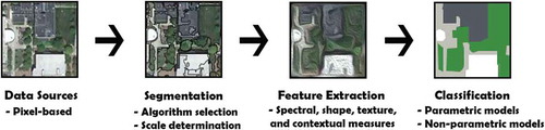
The objective of this paper is to summarize the emerging trends in GEOBIA and discuss potential opportunities as this paradigm evolves. Our intention is not to provide a comprehensive review of the theoretical foundations and typical algorithms in GEOBIA, which is already available in the literature (e.g., Hay and Castilla 2008; Blaschke 2010; Chen et al. 2012a; Blaschke et al. 2014; Ma et al. 2017b). Rather, we wish to detect emerging trends in the literature and to suggest new research opportunities by synthesizing advances across multiple subfields of GEOBIA. To determine the emerging trends, we reviewed the literature describing GEOBIA research directions and algorithms published over the past decade. We used the classic GEOBIA framework (Figure 1) to guide our review and scrutinized new developments in multiple subfields. While some topics had been brought out in the early years of GEOBIA, they resurged in recent years and are thus included in this review too. The remainder of this paper is organized to describe the new developments in data sources (Section 2), image segmentation (Section 3), object-based feature extraction (Section 4), and geo-object-based modeling frameworks (Section 5), which are followed by a discussion about opportunities for future research (Section 6) and conclusions (Section 7).

2. Data sources

Since the late 1990s and early 2000s, the advent of high-spatial resolution (H-res’) satellite sensors offered the remote sensing community increasing flexibility to study fine-scale geographic entities or phenomena, almost anywhere on the Earth’s surface. A variety of sensors joined this growing H-res’ satellite fleet from the earlier IKONOS and QuickBird, to the more recent WorldView-3 with a 0.31-m resolution panchromatic band (DigitalGlobe, Colorado, USA). While early GEOBIA research primarily involved working with classic, single-image optical scenes for proof-of-concept studies, more recent developments have shown new trends of an increased use of nontraditional data types with richer spectral, spatial, and temporal information, as well as data fusion and integration for improved modeling of geographic entities or phenomena. Here, we define the “traditional” GEOBIA data as H-res’ (typically finer than 5 m) imagery, which is acquired by remote sensors mounted on relatively stable satellite/airborne platforms and contains a limited number of spectral bands, i.e., low spectral resolution.

2.1. Nontraditional data types

2.1.1. UAS/Drones

The data typically used in GEOBIA are optical imagery acquired by satellite or airborne sensors. However, one of their challenges involves data acquisition flexibility. Operating aircrafts is often subject to rigorous aviation regulations and weather conditions; meanwhile, satellite sensors have predefined orbits and revisit intervals that are difficult to alter. UAS (or drones) as a relatively recent aerial platform have an ability to collect submeter or sub-decimeter resolution data (Figure 2) with a high flexibility and a reduced demand for resources (see a review by Colomina and Molina (2014)). Such platforms are particularly effective for capturing a rapid or unexpected change in geographic objects, where a fast response is desired, such as early season weed detection for precision agriculture (Torres-Sánchez, López-Granados, and Peña 2015; Pérez-Ortiz et al. 2016), post-disaster structural damage assessment (Fernandez-Galarreta, Kerle, and Gerke 2015), and extraction of detailed vegetation species types for rangeland monitoring (Laliberte and Rango 2011). Although UAS platforms come in a variety of sizes, shapes, and flight-time capacities, they are typically appropriate only for projects of limited spatial coverage. Additionally, their operation has to meet specific safety and privacy regulations that vary considerably across nations and states. In real-world applications, however, UASs have been shown to be effective for extending or replacing plot-level field observations (e.g., land-cover type and air quality monitoring; Watts, Ambrosia, and Hinkley 2012). Consequently, the integration of UAS and GEOBIA technologies represents a flexible and economically appealing means to augment ground-truth data, which is typically time consuming and costly to acquire.

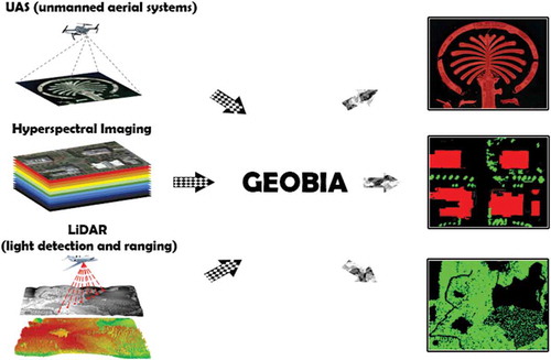
Figure 2. Nontraditional data types and image-objects.

2.1.2. Hyperspectral imagery

Hyperspectral imagery (with dozens to hundreds of spectral bands) has been increasingly adopted by GEOBIA practitioners to distinguish between geographic objects of similar spectral characteristics. This is because traditionally, H-res’ imagery is limited in spectral discrimination, comprising only a few bands that typically span the visible to near-infrared portions of the electromagnetic spectrum. Examples of GEOBIA projects using hyperspectral imaging include classifying mangrove species with 30-band CASI-2 data (Kamal and Phinn 2011), mapping crop types in precision agriculture using a 242-band Hyperion image (Petropoulos, Kalaitzidis, and Prasad Vadrevu 2012), assessing post-fire burn severity in a forested landscape utilizing a 50-band MASTER mosaic (Chen et al. 2015), and capturing tropical forest species diversity with the 129-band AisaEAGLE imaging spectrometer (Schäfer et al. 2016). Compared to multispectral data, hyperspectral imagery offers richer spectral information. This is particularly beneficial to GEOBIA because extra spectral bands may be used to generate a number of object-based shape, textural and contextual features, potentially improving the delineation of fine-scale geographic entities or phenomena. However, the exponentially increased feature space needs increased data storage and rigorous analysis for feature reduction, which is computationally intensive. It is also true that the majority of hyperspectral sensors, such as CASI, HyMap, and AVIRIS, are mounted on airborne platforms (Chen and Meentemeyer 2016). While it remains challenging for satellite sensors to achieve high-spectral and high-spatial resolution simultaneously, recent sensor technologies have advanced to collect spectral information beyond the typical red, green, blue, and near-infrared portions of the spectrum. For instance, Worldview-2 acquires additional coastal blue (400–450 nm), yellow (585–625 nm), red-edge (705–745 nm), and near-infrared-2 (860–1040 nm) bands at the 1.84-m resolution (DigitalGlobe, Colorado, USA). Novack et al. (2011) compared WorldView-2 (eight bands) with QuickBird-2 (four bands) using a GEOBIA framework in urban land-cover mapping. Their results indicated that the additional bands from WorldView-2 significantly improved model accuracy in 10 out of 16 tested classifications. Immitzer, Atzberger, and Koukal (2012) found a similar conclusion mapping tree species at the individual crown level in a mid-European forest site. They also reported improving the accuracy of species mapping with reflectance spectra from the SWIR (shortwave infrared) region, which is available in WorldView-3 (DigitalGlobe, Colorado, USA).

2.1.3. LiDAR (light detection and ranging)

LiDAR (light detection and ranging) complements the traditional 2D spectral signatures of the landscape with 3D structural information (Figure 2). As segmentation in GEOBIA is typically applied to 2D imagery, LiDAR point clouds (discrete-return system) or waveforms (full-waveform system) have to be converted to raster-format image models (i.e., digital surface/elevation/terrain models – DSM, DEM, DTM) before they can be readily used in a GEOBIA framework. For example, Freeland et al. (2016) used LiDAR data to identify archeological construction mounds, whose unique features of circular/conical shape and specific elevation range were well captured by LiDAR DEM-generated objects. Instead of using a DEM, Tomljenovic, Tiede, and Blaschke (2016) applied a LiDAR-derived DSM to isolate above-ground features. Through segmentation and a slope-based classification, buildings were successfully extracted from the other solid, non-ground objects (e.g., rocks, cars, power lines, and residual thick vegetation). The GEOBIA community has taken further advantage of LiDAR’s penetration capacity, which is able to retrieve the 3D structure of nonsolid objects with gaps, such as trees. Jakubowski, Guo, and Kelly (2013) applied a CHM (canopy height model results from subtracting a DEM from a DSM) to delineate individual trees. Using the same GEOBIA framework, the authors found that this LiDAR approach more closely resembles real forest structure than using pan-sharpened WorldView-2 optical imagery at a 0.5-m resolution.

2.2. Data integration

Three main directions appear in the data integration in GEOBIA, including (1) large-area coverage, (2) historical data gap filling, and (3) integrating/fusing data from different sensors with complementary characteristics. While GEOBIA has been known to be capable of combining multisource datasets since the early 2000s (Blaschke, Burnett, and Pekkarinen 2004), the three directions become more apparent recently. This can be explained by the increased data sources and availability, and the growing popularity of GEOBIA in a wide variety of real-world applications.

2.2.1. Large-area coverage

Unlike medium, or low-spatial resolution data where each scene covers a large area (e.g., a swath of Landsat – 185 km), H-res’ sensors typically have a narrow swath width (e.g., 13.1 km for WorldView-3). As a result, a study area of interest is likely covered by multiple H-res’ images, acquired from different dates and/or various sensors. The variations in sensor look angle, solar elevation angle, atmospheric condition, and/or season may significantly affect accurate identification of geographic objects. For example, the same trees may show less sunlit and more shaded portions at a lower solar elevation angle (Wulder et al. 2008). As a result, the same set of segmentation parameters could result in variations of image-objects across the same type of land cover. Consequently, object-based features (e.g., shape or size) cannot hold the same significance level in a classification. While such an effect has been rarely evaluated and discussed in the literature, practical operations require cautious selection of data for consistent and transformative object-based analysis. Similarly, mosaicking H-res’ datasets can result in mosaic lines bisecting objects of interest from two or more times. In an effort to mitigate this issue using GEOBIA, Rahman et al. (2013) describe a novel GEOBIA algorithm referred to as Object-Based Mosaicing (OBM) that was used to automatically join 44 thermal airborne (TABI 1800) flight lines (covering 825 km² at 50 cm) around urban roof objects rather than bisecting them with arbitrary mosaic join lines. Without this solution, 14,209 roof objects (5% of the roofs in the scene) would have been bisected during the mosaic process resulting in very different hotspot detection results for these homes.

2.2.2. Historical data gap filling

The history of spaceborne H-res’ imaging is relatively brief with the majority of images acquired after 2000. Prior to this time, the pre-2000 data archives in many developed countries refer to aerial photos, which span most of the twentieth century. A recent trend is to integrate historical aerial photos with the latest satellite/airborne images to understand land-cover/use changes at fine scales over decades. For instance, Laliberte et al. (2004) used 11 aerial photos taken between 1937 and 1996, and a QuickBird image of 2003 to map shrub encroachment with GEOBIA. Similarly, Eitzel et al. (2016) estimated the long-term change of woody cover (1948–2009) by using historical black and white aerial images and more recent NAIP (national agricultural imagery program) data. Applying GEOBIA to accurately classify historical aerial photos is not an easy task, because they typically have a single band digitized from a film format, and they may also contain large geometric distortions. The lack of historical validation datasets (and/or knowledge of acquisition and camera parameters) poses further challenges for training and accuracy assessment. Additionally, GEOBIA projects that use time series data have tended to focus on mapping inter-annual land surface variation (e.g., crop growth between years). Intra-annual variation (e.g., such as crop growth or seasonal flood monitoring within a year) has yet to be well investigated with GEOBIA. Given the benefits of time series imagery, it is highly likely that dense time series data will soon become available and popular, as constellations of H-res’ satellites, microsatellites (wet mass: 10–100 kg), and nanosatellites (wet mass: 1–10 kg; SEI, 2014) have been or will be deployed by well-known or emerging commercial vendors (e.g., DigitalGlobe, Airbus Defence & Space, and Terra Bella).

2.2.3. Integrating/Fusing data from different sensors with complementary characteristics

While it is relatively trivial to extract meaningful objects when data are acquired from the same or similar sensors, it is also possible that the corresponding bands may not be sufficient for accurate analysis of those objects. Consequently, increasing efforts have been made to integrate various types of object-based features from multiple sensors. There are typically two ways to conduct such integration.

First, multisource data (e.g., optical, LiDAR, microwave, and thermal data) are combined to form one image file for segmentation. A prerequisite for this process is the conversion of all the data to a compatible raster format with the same spatial resolution and minimized geometric and atmospheric discrepancies. To avoid the possibility that one data source dominates in the creation of objects (unless desired), different weightings may be applied to different date sources. For example, classifying debris-covered glaciers may require a higher weight from topographic data (i.e., slope) than from optical and microwave imagery (Robson et al. 2015).

The second way is to generate image-objects using more traditional optical imagery. The object boundaries are then used as a constraint to extract object-based features from the other data types (e.g., Zhang, Xie, and Selch 2013; Godwin, Chen, and Singh 2015). For instance, Godwin, Chen, and Singh (2015) applied 1.0 m NAIP imagery to derive urban forest canopies at the crown and small tree cluster level. A range of LiDAR metrics (e.g., total return count, variance, and height percentiles) were calculated within the tree-objects for estimating urban forest carbon density. Accurate co-registration between multisource datasets is not trivial, but it is essential for successful object-based modeling, especially when objects are of small sizes. For example, Hay (2014) describes the integration of thermal and RGBi airborne datasets – acquired from different platforms, at different times, and spatial resolutions, with existing historical GIS roof polygons. In an effort to automatically link these very different data types – so as to exploit the best attributes of each – they have developed a proprietary (patent-pending) co-registration method referred to as Object-Based Geometric Fitting (Hay and Couloigner 2015). This method spatially superimposes a mask dataset comprising mask-objects on a raster image and locally superimposes individual mask-objects on individual image-objects, until all mask-objects are geometrically fitted to image-objects.

3. Image segmentation

Image segmentation acts as one of the key steps on which the performance of GEOBIA is critically dependent. The development of GEOBIA segmentation algorithms has long been influenced by Computer Vision, which has recognized the multiscale nature of geographic structures, e.g., small-scale residential homes versus large-scale commercial dwellings. It is also appreciated that a meaningful single scale is not possible to accurately segment the varied sized, shaped, and geographically located objects of interest in a remotely sensed image (Hay, Niemann, and Goodenough 1997; Marceau and Hay 1999). Rather, the optimal scale can vary with geographic entity or phenomenon, which possibly coexists within a single scene (Hay et al. 2001). Though scale optimization has been a topic of research for decades (Hay et al. 2002; Hay et al. 2003), more recent efforts (see below) have begun to address this issue with automatic, or semiautomatic “optimal” scale determination algorithms. Additionally, the GEOBIA community has recognized and benefited from the rapid development of computer vision and machine learning, attempting to directly partition imagery into semantically meaningful objects (a.k.a., semantic or supervised segmentation) with no need to conduct separate steps of object-based feature merging, extraction, and classification.

3.1. Scale parameter determination

While the human-driven, trial-and-error approach is popular to determine optimal scales, it is time-consuming and impractical for large-area applications (Im et al. 2014). The main idea behind automatic, scene-specific scale determination is the use of spectral, textural, shape, and/or contextual information of the images to define the “best” (a.k.a. most meaningful) object sizes and boundaries in an unsupervised manner. Such type of algorithms often relies on an optimization procedure (typically progressive or iterative) to refine the initially segmented results, or to select the optimal scale from a range of candidates. For example, thematic maps derived from image classification have been applied to improve multiscale segmentation and assist with scale selection (Troya-Galvis, Gançarski, and Berti-Équille 2017; Zhang, Xiao, and Feng 2017). Drǎguţ et al. (2014) proposed an iterative framework, which compared local variance (LV) from the same image at various segmentation levels. The optimal scale for segmentation was selected, if LV value at a given level was equal to or lower than the value recorded at the previous level which had a smaller scale parameter. Yang, He, and Weng (2015) argued that an optimal scale should enhance both the characteristics of intra-segment homogeneity and intersegment heterogeneity, which were calculated in a newly developed energy function. This function quantifies the relationship between each image-object and its neighboring objects using common boundary lengths as weights.

Since geographic entities and phenomena are almost never distributed following the same spatial patterns across a study site, an optimization procedure using global measures is likely to cause imbalanced performance (Yang, He, and Caspersen 2017). As a result, GEOBIA researchers have also applied local measures to guide splitting and/or merging the results from the initial segmentation (e.g., Hay et al. 2005; Martha et al. 2011; Chen et al. 2014b; Yang, He, and Caspersen 2017). Because splitting big objects involves repeated segmentation, the majority of researchers take a bottom-up approach which attempts to merge small objects (from an initial over-segmentation) until a stopping criterion is met. Typically, a local measure (e.g., variance or spectral distance) is calculated to quantify the relationship (i.e., similarity) between neighboring image-objects following each step of merging. A threshold parameter is used to define the similarity between image-objects and acts as the stopping criterion. The merging process terminates when the calculated local measure reaches the threshold. Despite great potential, this makes selecting an appropriate threshold critical to the success of high-quality segmentation, which may hinder the full automation of scale parameter determination. However, realistically, with many image-objects composing a scene, and not all image-objects being of interest, some researchers have used image-object size (within a defined range of minimum to maximum mappable units) as a kind of fuzzy, rather than a fixed threshold which has met with very useful results (Castilla, Hay, and Ruiz 2008; Castilla, Guthrie, and Hay 2009).

3.2. Semantic segmentation

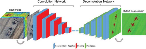
Unlike the classic unsupervised segmentation (e.g., region growing in eCognition; Baatz and Schape 2000), semantic segmentation is a supervised learning approach, from which each pixel is assigned a class label of its enclosing object (Long, Shelhamer, and Darrell 2015). As a learning-based framework, semantic segmentation has been significantly influenced by machine learning, with several groups of algorithms being proposed over the past decades, such as models using Markov random field (MRF; Feng, Jia, and Liu 2010; Zheng et al. 2013), and Bayesian network (BN; Zhang and Ji 2010). MRF is a type of probabilistic model that captures the contextual constraints within neighboring pixels, while BN can effectively quantify the relationships among image features. More recently, deep convolutional neural networks (CNNs; Krizhevsky, Sutskever, and Hinton 2012) have demonstrated superior performance in a range of digital image interpretation tasks, including geo-object detection from H-res’ imagery (e.g., Zhang, Zhang, and Du 2016; Wang et al. 2017a). In fact, CNNs – a particular kind of machine learning that is used to treat data as a nested hierarchy of concepts – are one of the most representative deep learning models (see Zhang, Zhang, and Du 2016, for a review of deep learning for remote sensing data analysis). Applying CNNs to semantic segmentation starts from raw imagery as input, where pixels pass through multiple layers and aggregate over progressively larger contextual neighborhoods, generating an object-based classification map as output (Marmanis et al. 2016). Figure 3 illustrates a typical workflow of CNNs, where three components are included – (1) convolutional and rectifier layers are used for feature extraction, (2) pooling function is to progressively reduce the spatial size of the representation reducing the number of parameters and computation in a network, and (3) prediction is the last step to assign each individual pixel a specific label class. Such end-to-end learning makes the classic object-based feature extraction obsolete, because local hierarchical features are learned by the stacked convolutional-pooling layers in CNNs (Krizhevsky, Sutskever, and Hinton 2012), thus reducing uncertainties in feature selection and improving automation in semantic labeling.

Figure 3. Workflow of deep convolutional neural networks (CNNs) for semantic segmentation.

While promising, semantic segmentation faces several challenges. For example, H-res’ imagery may lead to redundant/unnecessary details in some geographic objects (e.g., various roof materials in building objects, and complex within-crown structures in tree objects). Meanwhile, geo-objects are of multiple scales that are often within the extent of single image scenes. It is therefore challenging for semantic segmentation to combine features at different levels, as high-level and abstract features are appropriate for extracting large objects and low-level, raw features (e.g., an edge) are suitable for small objects (Wang et al. 2017a). Furthermore, deep learning models typically have a significant number of parameters for tuning, and the supervised learning fashion requires a large amount of reliable data for training.

4. Object-based feature extraction

Classic geo-object-based features include spectral, shape (geometric), texture, and contextual measures that are extracted following unsupervised image segmentation. Recent developments in GEOBIA, on the one hand, provide novel ways to capture features based on the characteristics of geographic objects. On the other hand, feature space reduction from a large pool of candidates has become an essential step and is increasingly relying on machine-learning approaches. These concepts will be discussed more fully in the proceeding subsections.

4.1. Novel object-based features

A classic direction of feature development focuses on characterizing attributes of individual image-objects (Figure 4), such as measuring shape complexity (Russ 2002; Jiao, Liu, and Li 2012), extracting interval features from interval-valued data modeling (He et al. 2016), and creating semivariogram descriptors to quantify the spatial correlation and patterns within objects (Balaguer et al. 2010; Powers et al. 2015). More recently, Wang et al. (2017b) extended their approach from individual image-objects to the relationship between objects and lines. Their hypothesis was that geographic objects in an urban setting tend to have more regular shapes, interacting with more systematically distributed lines than the natural environment. Thus, new features were proposed within a framework describing the object (region)-line relationship, i.e., region-line primitive association framework (RLPAF). Gil-Yepes et al. (2016) further suggested a temporal dimension for developing geostatistical features to examine the temporal behavior of each object’s internal structure, which were useful in object-based change detection (OBCD).

Figure 4. Object-based features extracted at three scales within (a) image-objects, (b) neighborhood image-objects, and (c) individual communities (e.g., urban blocks).

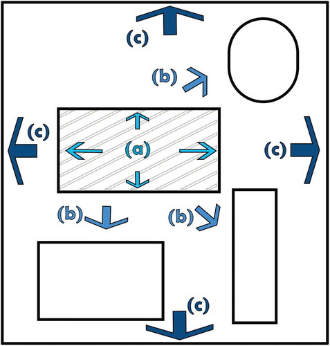
Another useful research direction involves improving the description of contextual information from neighboring image-objects (Hay and Niemann 1994; Hay, Niemann, and McLean 1996; Figure 4). Building on this earlier work, Chen et al. (2011) proposed geographic object-based image texture (GEOTEX), which treated each image-object and its neighbors as a natural window/kernel for calculating a new set of texture measures. By extension, Chen et al. (2017a) developed an object-based filtering algorithm, which improved land-cover mapping accuracy to study transitional landscape covered by a mixture of healthy trees, disease-impacted trees, shrubs, grass and bare ground. Conversely, rather than focusing on neighboring objects, Voltersen et al. (2014) assessed image-objects within each urban block and extracted their relationships at the block level (Figure 4). They calculated a total of 163 object-based features for buildings (e.g., number of buildings, and building aggregation), vegetation (vegetation fraction), 3D density (e.g., urban density), and landscape patterns (e.g., fractal dimension). The compact city structures of Berlin were well mapped with an overall accuracy of 82.1% (Voltersen et al. 2014).

Today’s remotely sensed data are of various characteristics from multiple sensors. Although image-objects may be derived from optical images, object-based features can also be calculated using other data sources located within the boundaries of image-objects, such as 3D topography (De Castilho Bertani, De Fátima Rossetti, and Albuquerque 2013), and LiDAR point clouds (Godwin, Chen, and Singh 2015). In such cases, accurate co-registration remains essential for meaningful feature extraction (Hay and Couloigner 2015), though image-objects are likely to have a higher geometric error tolerance than pixels (Chen et al. 2011; Chen, Zhao, and Powers 2014a).

While object-based features are typically calculated following segmentation, such a process typically generates a large number of features (in some GEOBIA software, upwards of 20× the original feature of interest), potentially reducing computation efficiency and increasing modeling uncertainties. This is especially true when hyperspectral imagery is used, as the number of corresponding object-based features can easily reach hundreds or thousands. In an effort to mitigate this issue, Chen et al. (2015) employed PCA (principal component analysis) and MNF (minimum noise fraction) to reduce the airborne MASTER sensor’s 50 input spectral bands prior to segmentation. The five new bands (or new features) from PCA and MNF demonstrated comparable performance in forest burn severity mapping, as compared to the use of all the 50 bands. This type of approach can also be considered as a means to reduce feature space.

4.2. Feature space reduction

Subjective selection of the salient features in GEOBIA is becoming increasingly impossible due to the large number of candidates derivable from a variety of object-based feature extraction methods. Efficient reduction of feature space (a.k.a., feature selection) includes a range of techniques from statistical analysis, to machine learning and deep learning. Most of these techniques are designed to follow the idea of maximizing the separation distances between classes while minimizing the number of input features. After processing, a ranking of features or feature combinations in order of significance is typically provided. As a standard function in the software eCognition, feature space optimization (FSO) is probably one of the most widely used statistical algorithms. Its goal is to select the best combination of features corresponding to the largest average minimum distance between the samples of different classes (Trimble 2014). However, popularity and ease of use do not always lead to a high accuracy in object-based classification. In a New Mexico’s semi-desert grassland study site, Laliberte, Browning, and Rango (2012) found that FSO produced the lowest accuracies in land-cover classification, when compared to the Jeffreys–Matusita distance and classification tree analysis (CTA) feature selection. Of those tested, CTA was deemed to be the best machine-learning approach, outperforming the other two statistical methods.

The popularity of machine-learning methods has grown for feature space reduction. In addition to high accuracy (e.g., Van Coillie, Verbeke, and De Wulf 2007; Pal and Foody 2010), many machine-learning algorithms are nonparametric; thus, they do not assume any specific distribution form for their observations, e.g., normality. In the GEOBIA community, however, consensus has yet to be reached in terms of which machine-learning algorithm(s) is superior to the others for particular applications. Recent studies have demonstrated the success of applying a variety of algorithms in object-based feature selection, such as winnow (Littlestone 1988; Powers et al. 2015), minimal redundancy maximal relevance (Peng, Long, and Ding 2005; Chen, Hay, and St-Onge 2012b), random forests (RF; Breiman 2001; Duro, Franklin, and Dubé 2012), and SVM (support vector machine) recursive feature elimination (Guyon et al. 2002; Huang and Zhang 2013). In our opinion, the popularity and utility of machine-learning algorithms depend on their performance (e.g., accuracy and processing time), ease of use (e.g., complexity of parameter tuning), and accessibility (e.g., embedded in commercial software or open-source programs). The algorithm selection of the optimal feature space reduction is also relevant to the use of the succeeding classification methods (if classification is the goal). For instance, RF was found to be relatively insensitive to the number of input features, while feature selection may have a higher impact on SVM (Ma et al. 2017a).

5. Geo-object-based modeling frameworks

Following the segmentation (or existing polygons) ⟶ feature extraction ⟶ classification framework (Blaschke et al. 2000), GEOBIA has primarily been used in land-cover/use classification. It has also recently been introduced to detect specific geographic objects of interests, such as archeological remains (Lasaponara et al. 2016), alluvial fans (Pipaud and Lehmkuhl 2017), dunes (Vaz et al. 2015), green roofs (Theodoridou et al. 2017), industrial disturbances (Powers et al. 2015), palm oil crowns (Chemura, Van Duren, and Van Leeuwen 2015), irrigated pasture (Shapero, Dronova, and Macaulay 2017), wild oat weed patches (Castillejo-González et al. 2014), illegal charcoal production (Bolognesi et al. 2015), tree species diversity (Schäfer et al. 2016), seagrass (Baumstark, Duffey, and Pu 2016), tropical successional stages (Piazza et al. 2016), wetland classes (Mui, He, and Weng 2015), invasive plants (Müllerová, Pergl, and Pyšek 2013), salt cedar (Xun and Wang 2015), paddy fields (Su 2017), urban heat-loss at the house, community and city scales (Hay et al. 2011), and roof object mosaicing (Rahman et al. 2013).

Since its initial introduction, this classic framework has been modified or extended in multiple ways to meet specific needs in real-world applications. One type of modification aims to use multiple classification steps to refine classification accuracy. For example, Eckert et al. (2017) applied classification results at a coarse scale to improve classification performance at a fine scale, based on the fact that some fine geographic objects only existed in certain landscape zones. Similarly, by using inner-object context to conduct a preliminary classification, Guo, Zhou, and Zhu (2013) employed a two-step strategy to refine classification using object-neighbor context (i.e., the characteristics of objects adjacent to the studied object) and scene context (i.e., the distribution of all the objects in the whole scene), respectively. While the majority of GEOBIA methods utilize image spectral information to study geographic objects, these methods often lack the capacity to analyze latent spatial phenomena. To address the challenge, Lang et al. (2008) defined geons as “spatial units that are homogenous in terms of varying space-time phenomena under policy concern.” Lang et al. (2014) further developed composite geons to represent functional land-use classes for regional planning purposes, and integrated geons to address abstract, yet policy-relevant phenomena such as societal vulnerability to hazards. Hofmann et al. (2015) extended the classic framework by coupling GEOBIA with the agent-based paradigm. They developed an agent-based image analysis framework for the purposes of automating the adaptation and adjusting rule sets in geo-object-based modeling.

While understanding what an object is (i.e., classification) remains crucial, GEOBIA researchers are increasingly focusing on the subtle variation(s) across the same classes of geographic objects. This type of framework still relies on the basic principles of geo-object-based modeling to derive image-object classes. However, its major advancement is the extension of the classic GEOBIA workflow by adding parametric (e.g., statistical and physically based) or nonparametric (e.g., machine learning) models to capture object-based variation within a specific class. For instance, Hultquist, Chen, and Zhao (2014) estimated forest burn severity at the small tree cluster level by comparing three machine-learning algorithms – Gaussian process regression, RFs, and support vector regression. Ozelkan, Chen, and Ustundag (2016) used linear regression models to map drought effects within rainfed and irrigated agricultural patches. Similarly, to calculate post-disaster urban structural damage, Fernandez-Galarreta, Kerle, and Gerke (2015) applied an object-based classification to extract small objects of damage features (e.g., cracks and holes) which were upscaled to the building level for accurate damage assessment. More recently, object-based variation was further extended to the temporal domain using time-series imagery. This type of OBCD emphasizes changes within individual classes, rather than class shifts from one to another. Examples include estimating stand ages of secondary vegetation succession (Fujiki et al. 2016), and monitoring earthquake-caused damage on man-made objects (De Alwis Pitts and So 2017).

A key differentiation between classic pixel-based approaches and GEOBIA is that GEOBIA incorporates the wisdom of the user into its frameworks, i.e., it uses semantics to translate image-objects into real-world features (Blaschke and Strobl 2001). While it is true that classic Bayesian and maximum likelihood classifiers allow for a limited (statistical) refinement of class rules, GEOBIA semantics are far customizable allowing for sophisticated rule sets to define and classify image-objects. This leads to a major strength of GEOBIA – transferability (Walker and Blaschke 2008; Kohli et al. 2013; Hamedianfar and Shafri 2015). Within the GEOBIA community, it is widely believed that this strength is mainly associated with the fuzzy concept (Hofmann, Blaschke, and Strobl 2011; Belgiu, Drǎguţ, and Strobl 2014; Hofmann 2016). However, user-driven selection of GEOBIA algorithms (e.g., in segmentation) and parameters (e.g., scale) within the same framework may differ significantly from one user to another for defining the same objects of interest, mainly due to users’ diverse backgrounds and experiences. To facilitate effective knowledge exchange and management, the GEOBIA community has started to embrace ontologies and develop ontology-driven models (Arvor et al. 2013; Blaschke et al. 2014; Gu et al. 2017; Baraldi 2017). The term “ontology” in information science is broadly defined as an explicit specification of a conceptualization (Gruber 1993). Instead of starting with the identification of specific objects (e.g., buildings), ontology-based modeling explicitly conceptualizes the real world using consensual knowledge (e.g., a national land cover classification system) in a way that is machine understandable (e.g., using ontology languages). Despite the important role of ontologies in GEOBIA, until recently, there remains a lack of comprehensive and widely accepted GEOBIA frameworks in which expert knowledge is formalized with ontologies. Having said this, the same can also be said for the entire field of remote sensing in general.

6. Opportunities

6.1. Big data challenge

H-res’ remotely sensed data are becoming increasingly available as we enter the big data era. While it is still debatable how remote-sensing data can be used as a type of big data, there is no doubt that daily sensors are acquiring massive amounts of data and that these data provide improved spectral, spatial, and temporal coverage of the landscape, resulting in a remarkable amount of detail for modeling the real-world. Though not solved, the GEOBIA community is well aware of this challenge. In efforts to mitigate big data volumes, recent research emphasis has been placed on automating GEOBIA algorithms, e.g., automatic scale parameter determination and the incorporation of machine learning (see reviews in previous sections). However, we suggest that an opportunity exists to develop tools that provided users with an “automatic” selection of data of appropriate resolution for specific questions of interest. For example, there are a wide range of image resolutions typically used by GEOBIA practitioners from 1000+ m to 0.3 m. Meanwhile, geographic objects within a scene are of various sizes, shapes, and spatial arrangement – for example ranging from leaves to small trees, to major shopping centers, and cities. At present, it is largely up to GEOBIA practitioners’ own discretion to choose an appropriate data type and resolution for a specific classification task in a study area covered by certain geographic objects. Though it may be considered “standard practice” to use high-resolution imagery to delineate large objects, too much spatial detail for the geographic objects of interest may not necessarily lead to high modeling accuracies (e.g., Müllerová, Pergl, and Pyšek 2013; Chen et al. 2017b). In addition, high-resolution data remain relatively costly and for large areas will require multiple datasets typically acquired at different times, with different illumination and atmospheric conditions – along with the related challenges involved in mosaicking these data. We suggest that new criteria are needed to fill the gap between data products and GEOBIA practitioners’ needs, so as to support timely, cost-effective, and useful data acquisitions. Here, such criteria could be incorporated into a semantic online system, such as a recent data querying system designed and implemented by Tiede et al. (2017). Through incorporating semantic queries and rules, such a system could assist users to make informed decisions in terms of what type(s) of data are more likely to meet specific project needs, such as data availability, pre/post-processing requirements, costs, and suitability for modeling certain geographic objects over space and time.

6.2. New forms of image-objects

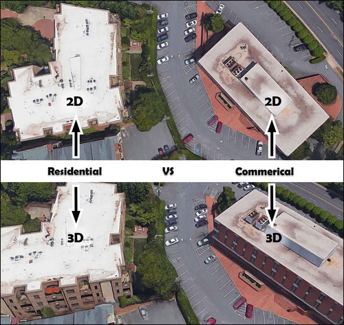
Image-objects are 2D representations of 3D geographic objects (e.g., buildings and trees) that exist within, and/or over time. Neglecting one spatial dimension could introduce uncertainties and errors in identifying ground features. For example, patches of trees and shrubs (in 2D) may reveal similar spectral and spatial characteristics, which can be better distinguished using their vertical structure (i.e., 3D, Alexander et al. 2010). Residential and commercial buildings in areas of mixed-use development tend to have comparable roof shapes and building materials; however, the distinctive patterns of their windows, doors, or texts/signs in building façades could act as salient features to improve classification (Li, Zhang, and Li 2017; Figure 5). With advances in remote sensing and computer vision, capturing geographic objects in 3D at H-res’ becomes an increasingly achievable task. In fact, GEOBIA researchers have started incorporating the vertical features in GEOBIA modeling, e.g., carbon estimation at the tree-cluster level using canopy height from a LiDAR sensor (Godwin, Chen, and Singh 2015). However, object-based features in these studies were typically calculated within the boundaries of 2D image-objects (e.g., Zhang, Xie, and Selch 2013; Godwin, Chen, and Singh 2015). Wouldn’t it make more sense to generate image-object features directly from a 3D scene-model, which is a more accurate representation of real-world geographic objects? The 3D scene-models can be constructed by using photogrammetry and computer vision techniques (Luhmann et al. 2013), in particular, the fusion of LiDAR and optical data in an automatic or semiautomatic fashion (see a review by Wang 2013).

Figure 5. Residential versus commercial buildings from 2D to 3D (image credit: Google Map©).

Unfortunately, precisely delineating object boundaries, even with the assistance of 3D information, remains challenging. It is actually possible that crisp boundaries may not exist for certain scene components such as a transitional zone between wetland and water (Bian 2007). Under such circumstances, forcing image-objects to have clearly defined boundaries is challenging and potentially misleading. Here, defining fuzzy boundaries provides a potential solution. An image-object is traditionally interpreted as an internally homogenous unit, where all parts of an object have an equal possibility of belonging to a certain class. Compared to the object center, however, the boundary (i.e., edge) areas are more likely to be misclassified. To mitigate this, it may be better to model this situation if object boundaries can demonstrate a graded change in probability, using sub-objects derived at a smaller scale. In early research, Hay et al. (2001) referred to these boundary components as edge-objects.

6.3. GEOBIA systems for novice-GEOBIA users

After almost two decades of development (Blaschke et al. 2014), the GEOBIA paradigm, frameworks, and software packages have been increasingly recognized by the GIScience community and many other fields. While GEOBIA experts often take advantage of the paradigm’s capacity to incorporate user’s knowledge and experience to achieve high modeling accuracies, novice-GEOBIA users are more likely to rely on default algorithms and parameters to complete the process without appropriately using semantics. To promote a wider application of GEOBIA, an ideal system should allow novice-GEOBIA users to easily translate their understandings of the geographic entities or phenomena of interest into an appropriate choice of algorithms and parameters. This system should be intuitive, interactive and efficiently respond to the user’s needs. The architecture of such a system may be designed to include three components: (1) data query, (2) a processing chain, and (3) product sharing, which can interactively direct a user to go through the entire GEOBIA process. To facilitate the translation from the novice-GEOBIA user to GEOBIA language, rule sets may be defined and trained by machine learning, or more recently deep learning algorithms that have achieved great success making data-driven decisions or predictions (Kotsiantis 2007; Krizhevsky, Sutskever, and Hinton 2012). Alternatively, GEOBIA software could begin compiling statistics (a.k.a. user analytics) on how users solve specific GEOBIA challenges. These results and method-flow could then be linked and shared with many 1000s of others to compile a set of best practices, or recipes/guides for creating specific outcomes.

6.4. Incorporating knowledge from other disciplines

While GEOBIA has been widely used to generate baseline data (e.g., land-cover/use maps) supporting studies in a variety of disciplines (e.g., forestry, urban planning; see examples in Section 5), much work remains regarding how well these disciplines can effectively support geo-object-based modeling. Due to the nature of image analysis, GEOBIA benefits greatly from knowledge advances in the image domain, e.g., computer vision that simulates human perception of digital imagery (Blaschke et al. 2014). However, improper (or insufficient) spatial, spectral, or temporal resolution may cause computer programs or even experienced photo interpreters to have biased or incorrect perceptions of geographic entities or phenomena (Hay and Castilla 2008). To mitigate such effects, it is essential to take advantage of the Earth-centric nature of GEOBIA (Hay and Castilla 2008), where the observed geo-objects and their spatiotemporal dynamics meet specific rules or laws in natural or built environments. For instance, different types of urban structures may show similar image characteristics (e.g., tones and shape) at the single building-object level, although the spatial co-occurrence between these structures (i.e., knowledge from urban planning) may reveal distinct patterns (and novel object-based features) at the block level (Voltersen et al. 2014). Similarly, in the vegetation transitional zone from dense forest to bare ground in California, Chen et al. (2017a) employed a classic GEOBIA framework to map disease-caused tree mortality and found that patches of dead trees were consistently overestimated due to similar spectral, textural, and geometrical characteristics between dead tree crowns and ground/shrubs/grass. To reduce mapping uncertainties, the spatial distribution patterns of disease – as a function of abiotic conditions (i.e., ecological species distribution modeling; Elith and Leathwick 2009) – may effectively constrain a geo-object-based model by informing the likelihood that disease disturbances may or may not occur at specific locations. Unfortunately, many recent GEOBIA studies have not exploited similar knowledge from non-image-based disciplines (e.g., urban planning, spatial ecology, and archeology). We suggest that incorporating such knowledge within geo-object-based modeling needs to be seriously considered to take full advantage of GEOBIA’s potential.

7. Conclusions

In this paper, we have presented a review of the emerging trends in GEOBIA over the last decade and have suggested new research opportunities by synthesizing advances across multiple GEOBIA subfields. As the theoretical foundations of GEOBIA have rapidly grown out of its infancy, recent studies have revealed an evident research shift toward the improvement of GEOBIA algorithms, aiming at more accurate, automatic, transformative, and computationally efficient frameworks. This trend is expected to continue with the incorporation of new data types from remote sensing and the “new” knowledge from multiple disciplines that are image based (e.g., computer vision, and machine learning) and Earth centric (e.g., urban planning, and spatial ecology). While such a large pool of data and algorithms may hold promise for meaningful geo-object-based modeling, it is also challenging for GEOBIA practitioners to choose an optimal data-algorithm combination that can address accurately a specific mapping problem. We suggest that new GEOBIA developments which can access and harness “the wisdom of the crowd” and/or the “experience of the GEOBIA community” are desired to support informed and efficient decision-making by both researchers and practitioners.

Disclosure statement

No potential conflict of interest was reported by the authors.

References

- Alexander, C., K. Tansey, J. Kaduk, D. Holland, and N. J. Tate. 2010. “Backscatter Coefficient as an Attribute for the Classification of Full-Waveform Airborne Laser Scanning Data in Urban Areas.” ISPRS Journal of Photogrammetry and Remote Sensing 65: 423–432. doi:10.1016/j.isprsjprs.2010.05.002.
- Arvor, D., L. Durieux, S. Andrés, and M. A. Laporte. 2013. “Advances in Geographic Object-Based Image Analysis with Ontologies: A Review of Main Contributions and Limitations from a Remote Sensing Perspective.” ISPRS Journal of Photogrammetry and Remote Sensing 82: 125–137. doi:10.1016/j.isprsjprs.2013.05.003.
- Baatz, M., and A. Schape. 2000. “Multiresolution Segmentation - an Optimization Approach for High Quality Multi-Scale Image Segmentation.” In Angewandte Geographische Informations- Verarbeitung XII, edited by J. Strobl, T. Blaschke, and G. Griesebner, 12–23. Karlsruhe, Germany: Wichmann Verlag.
- Balaguer, A., L. A. Ruiz, T. Hermosilla, and J. A. Recio. 2010. “Definition of a Comprehensive Set of Texture Semivariogram Features and Their Evaluation for Object-Oriented Image Classification.” Computers & Geosciences 36: 231–240. doi:10.1016/j.cageo.2009.05.003.
- Baraldi, A. 2017. “Pre-processing, Classification and Semantic Querying of Large-scale Earth Observation Spaceborne/Airborne/Terrestrial Image Databases: Process and Product Innovations.” Unpublished PhD Thesis. University of Naples “Federico II”, Italy, pp 519.
- Baumstark, R., R. Duffey, and R. Pu. 2016. “Mapping Seagrass and Colonized Hard Bottom in Springs Coast, Florida Using WorldView-2 Satellite Imagery.” Estuarine, Coastal and Shelf Science 181: 83–92. doi:10.1016/j.ecss.2016.08.019.
- Belgiu, M., L. Drǎguţ, and J. Strobl. 2014. “Quantitative Evaluation of Variations in Rule-Based Classifications of Land Cover in Urban Neighbourhoods Using WorldView-2 Imagery.” ISPRS Journal of Photogrammetry and Remote Sensing 87: 205–215. doi:10.1016/j.isprsjprs.2013.11.007.
- Bian, L. 2007. “Object-Oriented Representation of Environmental Phenomena: Is Everything Best Represented as an Object?” Annals of the Association of American Geographers 97: 267–281. doi:10.1111/j.1467-8306.2007.00535.x.
- Blaschke, T. 2010. “Object Based Image Analysis for Remote Sensing.” Journal of Photogrammetry and Remote Sensing 65: 2–16. doi:10.1016/j.isprsjprs.2009.06.004.
- Blaschke, T., C. Burnett, and A. Pekkarinen. 2004. “Image Segmentation Methods for Object-Based Analysis and Classification.” In Remote Sensing Image Analysis: Including the Spatial Domain, edited by F. De Meer and S. De Jong, 211–236. Dordrecht: Kluver Academic Publishers.
- Blaschke, T., G. J. Hay, M. Kelly, S. Lang, P. Hofmann, E. Addink, R. Q. Feitosa, et al. 2014. “ISPRS Journal of Photogrammetry and Remote Sensing Geographic Object-Based Image Analysis – Towards a New Paradigm.” ISPRS Journal of Photogrammetry and Remote Sensing 87: 180–191. doi:10.1016/j.isprsjprs.2013.09.014.
- Blaschke, T., and J. Strobl. 2001. “What’s Wrong with Pixels? Some Recent Developments Interfacing Remote Sensing and GIS.” GIS–Zeitschrift Für Geoinformationssysteme 14: 12–17.
- Blaschke, T., S. Lang, E. Lorup, J. Strobl, and P. Zeil. 2000. “Object-Oriented Image Processing in an Integrated GIS/remote Sensing Environment and Perspectives for Environmental Applications.” In Environmental Information for Planning, Politics and the Public, edited by A. Cremers and K. Greve, 555–570. Vol. 2. Marburg: Metropolis.
- Bolognesi, M., A. Vrieling, F. Rembold, and H. Gadain. 2015. “Rapid Mapping and Impact Estimation of Illegal Charcoal Production in Southern Somalia Based on WorldView-1 Imagery.” Energy for Sustainable Development 25: 40–49. doi:10.1016/j.esd.2014.12.008.
- Breiman, L. 2001. “Random Forests.” Machine Learning 45: 5–32. doi:10.1023/A:1010933404324.
- Castilla, G., G. J. Hay, and J. R. Ruiz. 2008. “Size-Constrained Region Merging (SCRM): An Automated Delineation Tool for Assisted Photointerpretation.” Photogrammetric Engineering & Remote Sensing 74: 409–419. doi:10.14358/PERS.74.4.409.
- Castilla, G., and G. J. Hay. 2008. “Image-Objects and Geographic Objects.” In Object-Based Image Analysis, edited by T. Blaschke, S. Lang, and G. Hay, 91–110. Heidelberg, Berlin, New York: Springer.
- Castilla, G., R. Guthrie, and G. J. Hay. 2009. “The Landcover Change Mapper (LCM) and Its Applications to Timber Harvest Monitoring in Western Canada.” Special Issue on Landcover Change Detection for Photogrammetric Engineering & Remote Sensing 75: 941–950. doi:10.14358/PERS.75.8.941.
- Castillejo-González, I. L., J. M. Peña-Barragán, M. Jurado-Expósito, F. J. Mesas-Carrascosa, and F. López-Granados. 2014. “Evaluation of Pixel- and Object-Based Approaches for Mapping Wild Oat (Avena Sterilis) Weed Patches in Wheat Fields Using QuickBird Imagery for Site-Specific Management.” European Journal of Agronomy 59: 57–66. doi:10.1016/j.eja.2014.05.009.
- Chemura, A., I. Van Duren, and L. M. Van Leeuwen. 2015. “Determination of the Age of Oil Palm from Crown Projection Area Detected from WorldView-2 Multispectral Remote Sensing Data: The Case of Ejisu-Juaben District, Ghana.” ISPRS Journal of Photogrammetry and Remote Sensing 100: 118–127. doi:10.1016/j.isprsjprs.2014.07.013.
- Chen, G., E. Ozelkan, K. K. Singh, J. Zhou, M. R. Brown, and R. K. Meentemeyer. 2017b. “Uncertainties in Mapping Forest Carbon in Urban Ecosystems.” Journal of Environmental Management 187: 229–238. doi:10.1016/j.jenvman.2016.11.062.
- Chen, G., G. J. Hay, and B. St-Onge. 2012b. “A GEOBIA Framework to Estimate Forest Parameters from Lidar Transects, Quickbird Imagery and Machine Learning: A Case Study in Quebec, Canada.” International Journal of Applied Earth Observation and Geoinformation 15: 28–37. doi:10.1016/j.jag.2011.05.010.
- Chen, G., G. J. Hay, G. Castilla, and B. St-Onge. 2011. “A Multiscale Geographic Object-Based Image Analysis to Estimate Lidar- Measured Forest Canopy Height Using Quickbird Imagery.” International Journal of Geographical Information Science 25: 877–893. doi:10.1080/13658816.2010.496729.
- Chen, G., G. J. Hay, L. M. T. Carvalho, and M. Wulder. 2012a. “Object-Based Change Detection.” International Journal of Remote Sensing 33: 4434–4457. doi:10.1080/01431161.2011.648285.
- Chen, G., K. Zhao, and R. Powers. 2014a. “Assessment of the Image Misregistration Effects on Object-Based Change Detection.” ISPRS Journal of Photogrammetry and Remote Sensing 87: 19–27. doi:10.1016/j.isprsjprs.2013.10.007.
- Chen, G., M. R. Metz, D. M. Rizzo, W. W. Dillon, and R. K. Meentemeyer. 2015. “Object-Based Assessment of Burn Severity in Diseased Forests Using High-Spatial and High-Spectral Resolution MASTER Airborne Imagery.” ISPRS Journal of Photogrammetry and Remote Sensing 102: 38–47. doi:10.1016/j.isprsjprs.2015.01.004.
- Chen, G., and R. K. Meentemeyer. 2016. “Remote Sensing of Forest Damage by Diseases and Insects.” In Remote Sensing for Sustainability, edited by Q. Weng, 145–162. Boca Raton, Florida: CRC Press, Taylor & Francis Group.
- Chen, G., Y. He, A. De Santis, G. Li, R. Cobb, and R. K. Meentemeyer. 2017a. “Assessing the Impact of Emerging Forest Disease on Wildfire Using Landsat and KOMPSAT-2 Data.” Remote Sensing of Environment 195: 218–229. doi:10.1016/j.rse.2017.04.005.
- Chen, J., M. Deng, X. Mei, T. Chen, Q. Shao, and L. Hong. 2014b. “Optimal Segmentation of a High-Resolution Remote-Sensing Image Guided by Area and Boundary.” International Journal of Remote Sensing 35: 6914–6939. doi:10.1080/01431161.2014.960617.
- Colomina, I., and P. Molina. 2014. “Unmanned Aerial Systems for Photogrammetry and Remote Sensing: A Review.” ISPRS Journal of Photogrammetry and Remote Sensing 92: 79–97. doi:10.1016/j.isprsjprs.2014.02.013.
- De Alwis Pitts, D. A., and E. So. 2017. “Enhanced Change Detection Index for Disaster Response, Recovery Assessment and Monitoring of Accessibility and Open Spaces (Camp Sites).” International Journal of Applied Earth Observation and Geoinformation 57: 49–60. doi:10.1016/j.jag.2016.12.004.
- De Castilho Bertani, T., D. De Fátima Rossetti, and P. C. G. Albuquerque. 2013. “Object-Based Classification of Vegetation and Terrain Topography in Southwestern Amazonia (Brazil) as a Tool for Detecting Ancient Fluvial Geomorphic Features.” Computers and Geosciences 60: 41–50. doi:10.1016/j.cageo.2013.06.013.
- Drǎguţ, L., O. Csillik, C. Eisank, and D. Tiede. 2014. “Automated Parameterisation for Multi-Scale Image Segmentation on Multiple Layers.” ISPRS Journal of Photogrammetry and Remote Sensing 88: 119–127. doi:10.1016/j.isprsjprs.2013.11.018.
- Duro, D. C., S. E. Franklin, and M. G. Dubé. 2012. “Multi-Scale Object-Based Image Analysis and Feature Selection of Multi-Sensor Earth Observation Imagery Using Random Forests.” International Journal of Remote Sensing 33: 4502–4526. doi:10.1080/01431161.2011.649864.
- Eckert, S., S. Tesfay Ghebremicael, H. Hurni, and T. Kohler. 2017. “Identification and Classification of Structural Soil Conservation Measures Based on Very High Resolution Stereo Satellite Data.” Journal of Environmental Management 193: 592–606. doi:10.1016/j.jenvman.2017.02.061.
- Eitzel, M. V., M. Kelly, I. Dronova, Y. Valachovic, L. Quinn-Davidson, J. Solera, and P. De Valpine. 2016. “Challenges and Opportunities in Synthesizing Historical Geospatial Data Using Statistical Models.” Ecological Informatics 31: 100–111. doi:10.1016/j.ecoinf.2015.11.011.
- Elith, J., and J. R. Leathwick. 2009. “Species Distribution Models: Ecological Explanation and Prediction across Space and Time.” Annual Reviews Ecology Evolution Systems 40: 677–697. doi:10.1146/annurev.ecolsys.110308.120159.
- Feng, W., J. Jia, and Z. Q. Liu. 2010. “Self-Validated Labeling of Markov Random Fields for Image Segmentation.” IEEE Transactions on Pattern Analysis and Machine Intelligence 32: 1871–1887. doi:10.1109/TPAMI.2010.24.
- Fernandez-Galarreta, J., N. Kerle, and M. Gerke. 2015. “UAV-based Urban Structural Damage Assessment Using Object-Based Image Analysis and Semantic Reasoning.” Natural Hazards and Earth System Sciences 15: 1087–1101. doi:10.5194/nhess-15-1087-2015.
- Freeland, T., B. Heung, D. V. Burley, G. Clark, and A. Knudby. 2016. “Automated Feature Extraction for Prospection and Analysis of Monumental Earthworks from Aerial LiDAR in the Kingdom of Tonga.” Journal of Archaeological Science 69: 64–74. doi:10.1016/j.jas.2016.04.011.
- Fujiki, S., K. I. Okada, S. Nishio, and K. Kitayama. 2016. “Estimation of the Stand Ages of Tropical Secondary Forests after Shifting Cultivation Based on the Combination of WorldView-2 and Time-Series Landsat Images.” ISPRS Journal of Photogrammetry and Remote Sensing 119: 280–293. doi:10.1016/j.isprsjprs.2016.06.008.
- Gil-Yepes, J. L., L. A. Ruiz, J. A. Recio, Á. Balaguer-Beser, and T. Hermosilla. 2016. “Description and Validation of a New Set of Object-Based Temporal Geostatistical Features for Land-Use/Land-Cover Change Detection.” ISPRS Journal of Photogrammetry and Remote Sensing 121: 77–91. doi:10.1016/j.isprsjprs.2016.08.010.
- Godwin, C., G. Chen, and K. K. Singh. 2015. “The Impact of Urban Residential Development Patterns on Forest Carbon Density: An Integration of LiDAR, Aerial Photography and Field Mensuration.” Landscape and Urban Planning 136: 97–109. doi:10.1016/j.landurbplan.2014.12.007.
- Gruber, T. R. 1993. “Toward Principles for the Design of Ontologies Used for Knowledge Sharing”. In N. Guarino and R. Poli, editors, Proceedings of the International Workshop on Formal Ontology in Conceptual Analysis and Knowledge Representation, Kluwer Academic Publishers, Dordrecht, The Netherlands.
- Gu, H., H. Li, L. Yan, Z. Liu, T. Blaschke, and U. Soergel. 2017. “An Object-Based Semantic Classification Method for High Resolution Remote Sensing Imagery Using Ontology.” Remote Sensing 9: 329. doi:10.3390/rs9040329.
- Guo, J., H. Zhou, and C. Zhu. 2013. “Cascaded Classification of High Resolution Remote Sensing Images Using Multiple Contexts.” Information Sciences 221: 84–97. doi:10.1016/j.ins.2012.09.024.
- Guyon, I., J. Weston, S. Barnhill, and V. Vapnik. 2002. “Gene Selection for Cancer Classification Using Support Vector Machines.” Machine Learning 46: 389–422. doi:10.1023/A:1012487302797.
- Hamedianfar, A., and H. Z. M. Shafri. 2015. “Detailed Intra-Urban Mapping through Transferable OBIA Rule Sets Using WorldView-2 Very-High-Resolution Satellite Images.” International Journal of Remote Sensing 36: 3380–3396. doi:10.1080/01431161.2015.1060645.
- Hay, G. J. 2014. “GEOBIA: Evolving beyond Segmentation. Keynote Presentation. 5th GEOBIA International Conference.” 21–24 May, Thessaloniki, Greece – Accessed 30 Oct 2017. http://geobia2014.web.auth.gr/geobia14/sites/default/files/pictures/hay.pdf
- Hay, G. J., C. Kyle, B. Hemachandran, G. Chen, M. M. Rahman, T. S. Fung, and J. L. Arvai. 2011. “Geospatial Technologies to Improve Urban Energy Efficiency.” Remote Sensing 3: 1380–1405. doi:10.3390/rs3071380.
- Hay, G. J., D. J. Marceau, P. Dubé, and A. Bouchard. 2001. “A Multiscale Framework for Landscape Analysis: Object-Specific Analysis and Upscaling.” Landscape Ecology 16: 471–490. doi:10.1023/A:1013101931793.
- Hay, G. J., G. Castilla, M. A. Wulder, and J. R. Ruiz. 2005. “An Automated Object-Based Approach for the Multiscale Image Segmentation of Forest Scenes.” International Journal of Applied Earth Observation and Geoinformation 7: 339–359. doi:10.1016/j.jag.2005.06.005.
- Hay, G. J., and G. Castilla. 2008. “Geographic Object-Based Image Analysis (GEOBIA): A New Name for A New Discipline? Chapter 1. 4”In Object-Based Image Analysis – Spatial Concepts for Knowledge-Driven Remote Sensing Applications, edited by T. Blaschke, S. Lang, and G. J. Hay, 75–89.
- Hay, G. J., and I. Couloigner 2015. Patent: Methods and systems for object based geometric fitting. Canada. 21806_P48610US00_ProvisionalSB May 22.
- Hay, G. J., and K. O. Niemann. 1994. “Visualizing 3-D Texture: A Three-Dimensional Structural Approach to Model Forest Texture.” Canadian Journal of Remote Sensing 20: 90–101.
- Hay, G. J., K. O. Niemann, and D. G. Goodenough. 1997. “Spatial Thresholds, Image-Objects and Upscaling: A Multiscale Evaluation.” Remote Sensing of Environment 62: 1–19. doi:10.1016/S0034-4257(97)81622-7.
- Hay, G. J., K. O. Niemann, and G. McLean. 1996. “An Object-Specific Image-Texture Analysis of H-Resolution Forest Imagery.” Remote Sensing of Environment 55: 108–122. doi:10.1016/0034-4257(95)00189-1.
- Hay, G. J., P. Dubé, A. Bouchard, and D. J. Marceau. 2002. “A Scale-Space Primer for Exploring and Quantifying Complex Landscapes.” Ecological Modelling 153: 27–49. doi:10.1016/S0304-3800(01)00500-2.
- Hay, G. J., T. Blaschke, D. J. Marceau, and A. Bouchard. 2003. “A Comparison of Three Image-Object Methods for the Multiscale Analysis of Landscape Structure.” Photogrammetry and Remote Sensing 57: 327–345. doi:10.1016/S0924-2716(02)00162-4.
- He, H., T. Liang, D. Hu, and X. Yu. 2016. “Remote Sensing Clustering Analysis Based on Object-Based Interval Modeling.” Computers and Geosciences 94: 131–139. doi:10.1016/j.cageo.2016.06.006.
- Hofmann, P. 2016. “Defuzzification Strategies for Fuzzy Classifications of Remote Sensing Data.” Remote Sensing 8: 467. doi:10.3390/rs8060467.
- Hofmann, P., P. Lettmayer, T. Blaschke, M. Belgiu, S. Wegenkittl, R. Graf, T. J. Lampoltshammer, and V. Andrejchenko. 2015. “Towards a Framework for Agent-Based Image Analysis of Remote-Sensing Data.” International Journal of Image and Data Fusion 6: 115–137. doi:10.1080/19479832.2015.1015459.
- Hofmann, P., T. Blaschke, and J. Strobl. 2011. “Quantifying the Robustness of Fuzzy Rule Sets in Object-Based Image Analysis.” International Journal of Remote Sensing 32: 7359–7381. doi:10.1080/01431161.2010.523727.
- Huang, X., and L. Zhang. 2013. “An SVM Ensemble Approach Combining Spectral, Structural, and Semantic Features for the Classification of High-Resolution Remotely Sensed Imagery.” IEEE Transactions on Geoscience and Remote Sensing 51: 257–272. doi:10.1109/TGRS.2012.2202912.
- Hultquist, C., G. Chen, and K. Zhao. 2014. “A Comparison of Gaussian Process Regression, Random Forests and Support Vector Regression for Burn Severity Assessment in Diseased Forests.” Remote Sensing Letters 5: 723–732. doi:10.1080/2150704X.2014.963733.
- Im, J., L. J. Quackenbush, M. Li, and F. Fang. 2014. “Optimum Scale in Object-Based Image Analysis.” In Scale Issues in Remote Sensing, edited by Q. Weng. Hoboken, New Jersey: John Wiley & Sons.
- Immitzer, M., C. Atzberger, and T. Koukal. 2012. “Tree Species Classification with Random Forest Using Very High Spatial Resolution 8-Band worldView-2 Satellite Data.” Remote Sensing 4: 2661–2693. doi:10.3390/rs4092661.
- Jakubowski, M. K., Q. Guo, and M. Kelly. 2013. “Tradeoffs between Lidar Pulse Density and Forest Measurement Accuracy.” Remote Sensing of Environment 130: 245–253. doi:10.1016/j.rse.2012.11.024.
- Jiao, L., Y. Liu, and H. Li. 2012. “Characterizing Land-Use Classes in Remote Sensing Imagery by Shape Metrics.” ISPRS Journal of Photogrammetry and Remote Sensing 72: 46–55. doi:10.1016/j.isprsjprs.2012.05.012.
- Kamal, M., and S. Phinn. 2011. “Hyperspectral Data for Mangrove Species Mapping: A Comparison of Pixel-Based and Object-Based Approach.” Remote Sensing 3: 2222–2242. doi:10.3390/rs3102222.
- Kohli, D., P. Warwadekar, N. Kerle, R. Sliuzas, and A. Stein. 2013. “Transferability of Object-Oriented Image Analysis Methods for Slum Identification.” Remote Sensing 5: 4209–4228. doi:10.3390/rs5094209.
- Kotsiantis, S. 2007. “Supervised Learning: A Review of Classification Techniques.” Informatica 31: 249–268.
- Krizhevsky, A., I. Sutskever, and G. E. Hinton. 2012. “ImageNet Classification with Deep Convolutional Neural Networks.” Advances in Neural Information Processing Systems 25: 1106–1114.
- Laliberte, A. S., and A. Rango. 2011. “Image Processing and Classification Procedures for Analysis of Sub-Decimeter Imagery Acquired with an Unmanned Aircraft over Arid Rangelands.” GIScience & Remote Sensing 48: 4–23. doi:10.2747/1548-1603.48.1.4.
- Laliberte, A. S., A. Rango, K. M. Havstad, J. F. Paris, R. F. Beck, R. McNeely, and A. L. Gonzalez. 2004. “Object-Oriented Image Analysis for Mapping Shrub Encroachment from 1937 to 2003 in Southern New Mexico.” Remote Sensing of Environment 93: 198–210. doi:10.1016/j.rse.2004.07.011.
- Laliberte, A. S., D. M. Browning, and A. Rango. 2012. “A Comparison of Three Feature Selection Methods for Object-Based Classification of Sub-Decimeter Resolution UltraCam-L Imagery.” International Journal of Applied Earth Observation and Geoinformation 15: 70–78. doi:10.1016/j.jag.2011.05.011.
- Lang, S., P. Zeil, S. Kienberger, and D. Tiede. 2008. “Geons – Policy-Relevant Geo-Objects for Monitoring High-Level Indicators.” In Geospatial Crossroads @GI_Forum’ 08, edited by A. Car and J. Strobl, 180–186. Heidelberg: Wichmann.
- Lang, S., S. Kienberger, D. Tiede, M. Hagenlocher, and L. Pernkopf. 2014. “Geons-Domain-Specific Regionalization of Space.” Cartography and Geographic Information Science 41: 214–226. doi:10.1080/15230406.2014.902755.
- Lasaponara, R., G. Leucci, N. Masini, R. Persico, and G. Scardozzi. 2016. “Towards an Operative Use of Remote Sensing for Exploring the past Using Satellite Data: The Case Study of Hierapolis (Turkey).” Remote Sensing of Environment 174: 148–164. doi:10.1016/j.rse.2015.12.016.
- Li, X., C. Zhang, and W. Li. 2017. “Building Block Level Urban Land-Use Information Retrieval Based on Google Street View Images.” GIScience & Remote Sensing 54: 1–17. doi:10.1080/15481603.2017.1338389.
- Littlestone, N. 1988. “Learning Quickly When Irrelevant Attributes Abound: A New Linear-Threshold Algorithm.” Machine Learning 2: 285–318. doi:10.1007/BF00116827.
- Long, J., E. Shelhamer, and T. Darrell 2015. “Fully Convolutional Networks for Semantic Segmentation.” In Proceedings of the IEEE Conference on Computer Vision and Pattern Recognition. Boston, MA.
- Luhmann, T., S. Robson, S. Kyle, and J. Boehm. 2013. Close-Range Photogrammetry and 3D Imaging, 684. Berlin: De Gruyter.
- Ma, L., M. Li, X. Ma, L. Cheng, P. Du, and Y. Liu. 2017b. “A Review of Supervised Object-Based Land-Cover Image Classification.” ISPRS Journal of Photogrammetry and Remote Sensing 130: 277–293. doi:10.1016/j.isprsjprs.2017.06.001.
- Ma, L., T. Fu, T. Blaschke, M. Li, D. Tiede, Z. Zhou, X. Ma, and D. Chen. 2017a. “Evaluation of Feature Selection Methods for Object-Based Land Cover Mapping of Unmanned Aerial Vehicle Imagery Using Random Forest and Support Vector Machine Classifiers.” ISPRS International Journal of Geo-Information 6: 51. doi:10.3390/ijgi6020051.
- Marceau, D. J., and G. J. Hay. 1999. “Remote Sensing Contributions to the Scale Issue.” Canada Journal of Remote Sensing 25: 357–366. doi:10.1080/07038992.1999.10874735.
- Marmanis, D., J. D. Wegner, S. Galliani, K. Schindler, M. Datcu, and U. Stilla. 2016. “Semantic Segmentation of Aerial Images with an Ensemble of CNNs.” ISPRS Annals of Photogrammetry, Remote Sensing and Spatial Information Sciences III-3: 473–480. doi:10.5194/isprsannals-III-3-473-2016.
- Martha, T. R., N. Kerle, C. J. Van Westen, V. Jetten, and K. V. Kumar. 2011. “Segment Optimization and Data-Driven Thresholding for Knowledge-Based Landslide Detection by Object-Based Image Analysis.” IEEE Transactions on Geoscience and Remote Sensing 49: 4928–4943. doi:10.1109/TGRS.2011.2151866.
- Mui, A., Y. He, and Q. Weng. 2015. “An Object-Based Approach to Delineate Wetlands across Landscapes of Varied Disturbance with High Spatial Resolution Satellite Imagery.” ISPRS Journal of Photogrammetry and Remote Sensing 109: 30–46. doi:10.1016/j.isprsjprs.2015.08.005.
- Müllerová, J., J. Pergl, and P. Pyšek. 2013. “Remote Sensing as a Tool for Monitoring Plant Invasions: Testing the Effects of Data Resolution and Image Classification Approach on the Detection of a Model Plant Species Heracleum Mantegazzianum (Giant Hogweed).” International Journal of Applied Earth Observation and Geoinformation 25: 55–65. doi:10.1016/j.jag.2013.03.004.
- Novack, T., T. Esch, H. Kux, and U. Stilla. 2011. “Machine Learning Comparison between WorldView-2 and QuickBird-2-simulated Imagery regarding Object-Based Urban Land Cover Classification.” Remote Sensing 3: 2263–2282. doi:10.3390/rs3102263.
- Ozelkan, E., G. Chen, and B. B. Ustundag. 2016. “Spatial Estimation of Wind Speed: A New Integrative Model Using Inverse Distance Weighting and Power Law.” International Journal of Digital Earth 9: 733–747. doi:10.1080/17538947.2015.1127437.
- Pal, M., and G. M. Foody. 2010. “Feature Selection for Classification of Hyperspectral Data by SVM.” IEEE Transactions on Geoscience and Remote Sensing 48: 2297–2307. doi:10.1109/TGRS.2009.2039484.
- Peng, H., F. Long, and C. Ding. 2005. “Feature Selection Based on Mutual Information: Criteria of Max-Dependency, Max-Relevance, and Min-Redundancy.” IEEE Transactions on Pattern Analysis and Machine Intelligence 27: 1226–1238. doi:10.1109/TPAMI.2005.159.
- Pérez-Ortiz, M., J. M. Peña, P. A. Gutiérrez, J. Torres-Sánchez, C. Hervás-Martínez, and F. López-Granados. 2016. “Selecting Patterns and Features for Between- and Within- Crop-Row Weed Mapping Using UAV-imagery.” Expert Systems with Applications 47: 85–94. doi:10.1016/j.eswa.2015.10.043.
- Petropoulos, G. P., C. Kalaitzidis, and K. Prasad Vadrevu. 2012. “Support Vector Machines and Object-Based Classification for Obtaining Land-Use/Cover Cartography from Hyperion Hyperspectral Imagery.” Computers and Geosciences 41: 99–107. doi:10.1016/j.cageo.2011.08.019.
- Piazza, G. A., A. C. Vibrans, V. Liesenberg, and J. C. Refosco. 2016. “Object-Oriented and Pixel-Based Classification Approaches to Classify Tropical Successional Stages Using Airborne High-Spatial Resolution Images.” GIScience & Remote Sensing 53: 206–226. doi:10.1080/15481603.2015.1130589.
- Pipaud, I., and F. Lehmkuhl. 2017. “Object-Based Delineation and Classification of Alluvial Fans by Application of Mean-Shift Segmentation and Support Vector Machines.” Geomorphology 293: 178–200. doi:10.1016/j.geomorph.2017.05.013.
- Powers, R. P., T. Hermosilla, N. C. Coops, and G. Chen. 2015. “Remote Sensing and Object-Based Techniques for Mapping Fine-Scale Industrial Disturbances.” International Journal of Applied Earth Observation and Geoinformation 34: 51–57. doi:10.1016/j.jag.2014.06.015.
- Rahman, M. M., G. J. Hay, I. Couloigner, B. Hemachandaran, and J. Bailin. 2015. “A Comparison of Four Relative Radiometric Normalization (RRN) Techniques for Mosaicking H-Res Multi-Temporal Thermal Infrared (TIR) Flight-Lines of a Complex Urban Scene.” ISPRS Journal of Photogrammetry and Remote Sensing 106: 82–94. doi:10.1016/j.isprsjprs.2015.05.002.
- Rahman, M. M., G. J. Hay, I. Couloigner, B. Hemachandran, J. Bailin, Y. Zhang, and A. Tam. 2013. “Geographic Object-Based Mosaicing (OBM) of High-Resolution Thermal Airborne Imagery (TABI-1800) to Improve the Interpretation of Urban Image Objects.” IEEE Geoscience and Remote Sensing Letters 10: 918–922. doi:10.1109/LGRS.2013.2243815.
- Robson, B. A., C. Nuth, S. O. Dahl, D. Hölbling, T. Strozzi, and P. R. Nielsen. 2015. “Automated Classification of Debris-Covered Glaciers Combining Optical, SAR and Topographic Data in an Object-Based Environment.” Remote Sensing of Environment 170: 372–387. doi:10.1016/j.rse.2015.10.001.
- Russ, J. C. 2002. The Image Processing Handbook. 4th ed. Boca Raton, FL: CRC Press.
- Schäfer, E., J. Heiskanen, V. Heikinheimo, and P. Pellikka. 2016. “Mapping Tree Species Diversity of a Tropical Montane Forest by Unsupervised Clustering of Airborne Imaging Spectroscopy Data.” Ecological Indicators 64: 49–58. doi:10.1016/j.ecolind.2015.12.026.
- SEI (SpaceWorks Enterprises, Inc.). 2014. “Nano/Microsatellite Market Assessment.” http://www.sei.aero/eng/papers/uploads/archive/SpaceWorks_Nano_Microsatellite_Market_Assessment_January_2014.pdf.
- Shapero, M., I. Dronova, and L. Macaulay. 2017. “Implications of Changing Spatial Dynamics of Irrigated Pasture, California’s Third Largest Agricultural Water Use.” Science of the Total Environment, 605–606: 445–453. doi:10.1016/j.scitotenv.2017.06.065.
- Su, T. 2017. “Efficient Paddy Field Mapping Using Landsat-8 Imagery and Object-Based Image Analysis Based on Advanced Fractel Net Evolution Approach.” GIScience & Remote Sensing 54: 354–380. doi:10.1080/15481603.2016.1273438.
- Theodoridou, I., M. Karteris, G. Mallinis, E. Tsiros, and A. Karteris. 2017. “Assessing the Benefits from Retrofitting Green Roofs in Mediterranean, Using Environmental Modelling, {GIS} and Very High Spatial Resolution Remote Sensing Data: The Example of Thessaloniki, Greece.” Procedia Environmental Sciences 38: 530–537. doi:10.1016/j.proenv.2017.03.117.
- Tiede, D., A. Baraldi, M. Sudmanns, M. Belgiu, and S. Lang. 2017. “Architecture and Prototypical Implementation of a Semantic Querying System for Big Earth Observation Image Bases.” European Journal of Remote Sensing 50: 452–463.
- Tomljenovic, I., D. Tiede, and T. Blaschke. 2016. “A Building Extraction Approach for Airborne Laser Scanner Data Utilizing the Object Based Image Analysis Paradigm.” International Journal of Applied Earth Observation and Geoinformation 52: 137–148. doi:10.1016/j.jag.2016.06.007.
- Torres-Sánchez, J., F. López-Granados, and J. M. Peña. 2015. “An Automatic Object-Based Method for Optimal Thresholding in UAV Images: Application for Vegetation Detection in Herbaceous Crops.” Computers and Electronics in Agriculture 114: 43–52. doi:10.1016/j.compag.2015.03.019.
- Trimble. 2014. User Guide, 270 Trimble Inc., Sunnyvale, California, USA.
- Troya-Galvis, A., P. Gançarski, and L. Berti-Équille. 2017. “Remote Sensing Image Analysis by Aggregation of Segmentation-Classification Collaborative Agents.” Pattern Recognition 73: 259–274. doi:10.1016/j.patcog.2017.08.030.
- Van Coillie, F. M. B., L. P. C. Verbeke, and R. R. De Wulf. 2007. “Feature Selection by Genetic Algorithms in Object-Based Classification of IKONOS Imagery for Forest Mapping in Flanders, Belgium.” Remote Sensing of Environment 110: 476–487. doi:10.1016/j.rse.2007.03.020.
- Vaz, D. A., P. T. K. Sarmento, M. T. Barata, L. K. Fenton, and T. I. Michaels. 2015. “Object-Based Dune Analysis: Automated Dune Mapping and Pattern Characterization for Ganges Chasma and Gale Crater, Mars.” Geomorphology 250: 128–139. doi:10.1016/j.geomorph.2015.08.021.
- Voltersen, M., C. Berger, S. Hese, and C. Schmullius. 2014. “Object-Based Land Cover Mapping and Comprehensive Feature Calculation for an Automated Derivation of Urban Structure Types at Block Level.” Remote Sensing of Environment 154: 192–201. doi:10.1016/j.rse.2014.08.024.
- Walker, J. S., and T. Blaschke. 2008. “Object-Based Land-Cover Classification for the Phoenix Metropolitan Area: Optimization Vs. Transportability.” International Journal of Remote Sensing 29: 2021–2040. doi:10.1080/01431160701408337.
- Wang, H., Y. Wang, Q. Zhang, S. Xiang, and C. Pan. 2017a. “Gated Convolutional Neural Network for Semantic Segmentation in High-Resolution Images.” Remote Sensing 9: 1–15.
- Wang, M., Q. Cui, J. Wang, D. Ming, and G. Lv. 2017b. “Raft Cultivation Area Extraction from High Resolution Remote Sensing Imagery by Fusing Multi-Scale Region-Line Primitive Association Features.” ISPRS Journal of Photogrammetry and Remote Sensing 123: 104–113. doi:10.1016/j.isprsjprs.2016.10.008.
- Wang, R. 2013. “3D Building Modeling Using Images and LiDAR: A Review.” International Journal of Image and Data Fusion 4: 273–292. doi:10.1080/19479832.2013.811124.
- Watts, A. C., V. G. Ambrosia, and E. A. Hinkley. 2012. “Unmanned Aircraft Systems in Remote Sensing and Scientific Research: Classification and Considerations of Use.” Remote Sensing 4: 1671–1692. doi:10.3390/rs4061671.
- Wulder, M. A., J. C. White, N. C. Coops, and C. R. Butson. 2008. “Multi-Temporal Analysis of High Spatial Resolution Imagery for Disturbance Monitoring.” Remote Sensing of Environment 11: 2729–2740. doi:10.1016/j.rse.2008.01.010.
- Xun, L., and L. Wang. 2015. “An Object-Based SVM Method Incorporating Optimal Segmentation Scale Estimation Using Bhattacharyya Distance for Mapping Salt Cedar (Tamarisk Spp.) With QuickBird Imagery.” GIScience & Remote Sensing 52: 257–273. doi:10.1080/15481603.2015.1026049.
- Yang, J., Y. He, and J. Caspersen. 2017. “Region Merging Using Local Spectral Angle Thresholds: A More Accurate Method for Hybrid Segmentation of Remote Sensing Images.” Remote Sensing of Environment 190: 137–148. doi:10.1016/j.rse.2016.12.011.
- Yang, J., Y. He, and Q. Weng. 2015. “An Automated Method to Parameterize Segmentation Scale by Enhancing Intrasegment Homogeneity and Intersegment Heterogeneity.” IEEE Geoscience and Remote Sensing Letters 12: 1282–1286. doi:10.1109/LGRS.2015.2393255.
- Zhang, C., Z. Xie, and D. Selch. 2013. “Fusing Lidar and Digital Aerial Photography for Object-Based Forest Mapping in the Florida Everglades.” GIScience & Remote Sensing 50: 562–573.
- Zhang, L., and B. Du. 2016. “Deep Learning for Remote Sensing Data.” IEEE Geoscience and Remote Sensing Magazine 4: 22–40. doi:10.1109/MGRS.2016.2540798.
- Zhang, L., and Q. Ji. 2010. “Image Segmentation with a Unified Graphical Model.” IEEE Transactions on Pattern Analysis and Machine Intelligence 32: 406–1425.
- Zhang, X., P. Xiao, and X. Feng. 2017. “Toward Combining Thematic Information with Hierarchical Multiscale Segmentations Using Tree Markov Random Field Model.” ISPRS Journal of Photogrammetry and Remote Sensing 131: 134–146. doi:10.1016/j.isprsjprs.2017.08.003.
- Zheng, C., L. Wang, R. Chen, and X. Chen. 2013. “Image Segmentation Using Multiregion-Resolution MRF Model.” IEEE Xplore: IEEE Geoscience and Remote Sensing Letters 10: 816–820. doi:10.1109/LGRS.2012.2224842.