Object-wise joint-classification change detection for remote sensing images based on entropy query-by fuzzy ARTMAP

Abstract

The pixel-wise post-classification comparison (PCC) method is widely used in remote sensing images change detection. However, it is affected by the significant cumulative error caused by single image classification error. What’s more, the pixel-wise change detection method always produces “salt and pepper” effect. To solve the excessive evaluation of changed types and quantity caused by cumulative error and “salt and pepper” effect, a novel remote sensing image change detection method called entropy query-by fuzzy ARTMAP object-wise joint classification comparison (EQFAM-OBJCC) is presented in this article. Firstly, entropy query-by measurement of active learning is integrated with the fuzzy ARTMAP neural network to choose training samples which contain large amounts of information to improve the classification accuracy. Secondly, joint classification comparison is introduced to obtain the pixel-wise classification results. Finally, the object-wise classification and change detection results are produced by superpixel segmentation method, majority voting rule, and comparison of each superpixels. Experimental results demonstrate the validity of the proposed method. The classification and change detection results show that the proposed method can reduce the cumulative error with an average classification accuracy of 94.12% and a total detection error of 27.03%, and effectively resolve the “salt and pepper” problem. The proposed method was used to monitor the reclamation status of Liaohe estuary wetland via 10 time series remote sensing images from 1987 to 2014.

Keywords:

• change detection
• post-classification comparison
• fuzzy ARTMAP
• joint classification comparison
• superpixel segmentation

1. Introduction

Change detection of remote sensing images refers to the process of obtaining the change information using the comparison of remote sensing images in the same definite research region of different times (Li, Im, and Beier 2013). The accurate result of the change detection can improve the interpretation efficiency of the researchers on remote sensing images and has significant meaning for the dynamic monitoring of global change. The methods of the change detection can be broadly divided into two categories: the direct comparison method and the classification-based method (Chang et al. 2010). Both of them need accurate geometric registration of multi-temporal imagery because largely spurious results will be produced if there is misregistration (Berlanga-Robles and Ruiz-Luna 2011). The direct comparison method such as change vector analysis (CVA) (Marchesi, Bovolo, and Bruzzone 2010) is intuitive and easy to understand, but it requires more demanding preprocessing besides geometric registration, including accurate radiometric and atmospheric corrections (Hedjam et al. 2016). Direct comparison method directly compares spectral values or spectral features extracted from different temporal remote sensing images, then the comparison result is used to obtain the change detection result. Ghosh, Subudhi, and Bruzzone (2013) proposed a method using CVA which combined with Gibbs Markov random field to model the spatial regularity and obtained the difference between different temporal of images. Then, a modified Hopfield type neural network is exploited to estimate the maximum a posteriori probability. Ye, Chen, and Yu (2016) introduced support vector domain description into change vector analysis, which obtained high accuracy, especially for targeted change detection. However, it is easy to have spurious results in direct comparison methods (Zhu and Woodcock 2014), which is caused by inaccurate radiometric and atmospheric corrections, or unreasonable comparison thresholds. What’s more, it cannot provide a detailed change matrix for quantitative analysis.

Post-classification comparison (PCC) remains the most popular choices in classification-based change detection method (Peneva-Reed 2014). First, the two-temporal images, which are geometric corrected beforehand, can be classified separately using the same kind of classifier, and then the results of change detection can be obtained through the comparison of per-pixel. The parameters of the classifier are finely tuned according to their corresponding training samples. These kinds of methods are not constrained by atmospheric and environmental differences and have no need of other strict preprocessing. What’s more, it can obtain the classification information before and after the change. As the change detection accuracy obtained from the PCC method is approximated the product of independent classification accuracy theoretically, so the error of the independent classification will produce error accumulation, which can affect the accuracy of change detection significantly. In addition, PCC method needs effective training data for the detection of multiple change types.

It can be known from the aforementioned analysis that there are two main reasons that affect the accuracy of the PCC change detection (Lu et al. 2004). On the one aspect, variable imaging environment of remote sensing images may lead to the phenomenon that the same type of land cover has different spectral features. If multi-temporal images are separately classified, the classification of the same type of land cover may be easily misclassified (Hussain et al. 2013). Secondly, the PCC method which classified multi-temporal images separately will increase the false detection rate and generate accumulative error (Congalton et al. 2014). In addition, if the change area accounts for a little proportion of the total research area, then there will be a large number of repeat classification works in the no-change area, which will reduce the computational efficiency. Therefore, a well-behaved classification method needs to be seriously considered in PCC change detection.

Conventional classification methods often require the training samples to meet certain probability density distributions (Zhang, Chen, and Lu 2015). When the assumption is not satisfied, the classifiers may obtain poor performance, such as the maximum likelihood classifier (Otukei and Blaschke 2010). With the ability of self-learning and self-adaptive, neural network can solve the above shortcomings and assign explicit class label by collected supervised samples (Pal, Maxwell, and Warner 2013; Shao and Lunetta 2012; Voisin et al. 2014; Zhou, Lian, and Han 2016). Then applied to change detection, neural network can improve the separability of the changed and unchanged information (Chang et al. 2010). The fuzzy ARTMAP (FAM), which is developed from simple ART neural network, has the advantages of self-organization, fast speed learning, and complex mapping (Carpenter et al. 1992). What’s more, the FAM does not need to presuppose the probability density distribution of samples, and its structure can be adaptively adjusted when new training samples come. As a result, it has great advantages in the classification circumstance with complicated landcover types.

Generally, pixel-wise classifiers are most frequently utilized for remote sensing image classification. Although FAM is superior than many conventional classifiers, “salt and pepper” effect is likely to affect the classification accuracy when FAM is used to build simple pixel-wise classification, which shows as many noisy points in classification map. Object-wise classification methods regard a superpixel as a homogeneous object for joint classification. Each object in remote sensing image is composed of many connected neighborhood pixels with similar spectral and textural features and all pixels in an object are usually jointly classified and assigned to the same class (Liu et al. 2011; Levinshtein et al. 2009; Achanta et al. 2012). It can relieve the above problem and make the classification map conform to human visual perception, as well as reduce the complexity of the classification tasks. Object-wise classification method is now attracting more and more attention in the field of remote sensing image change detection (Hussain and Shan 2015).

The performance of classifier is also dependent on the quality of training samples. Generally, training samples for classification are generally collected by field survey and visual interpretation. The former is expensive and will cost more labor, and the latter is affected by the subjective factors. When the number of training samples is limited, active learning (AL) can firstly iteratively select a lot of valuable samples that contain most information for classification from an unlabeled candidate samples set, then assign labels to the selected samples to fill in the training sample set (Tuia, Pasolli, and Emery 2011; Zanotta et al. 2015). AL is an effective method to build a high-quality training sample set and to perform well in remote sensing classification and change detection.

To relieve the error accumulation problem in PCC change detection on two-temporal remote sensing images, an entropy query by fuzzy ARTMAP object-wise joint classification comparison (EQFAM-OBJCC) classification method is proposed. Firstly, AL method is integrated with the fuzzy ARTMAP neural network by choosing valuable training samples that contain most important information to improve the classification accuracy. Secondly, joint classification comparison (JCC) is introduced to reduce the error accumulation problem. A similarity matrix is constructed using spectral features to control the classification of the joint classifier. Pixel-wise joint classification results of two-temporal remote sensing images is obtained. Finally, entropy rate superpixel segmentation method is applied to obtain the boundary of each object. Object-wise classification results are obtained from pixel-wise classification results by the maximum voting. The object-wise change detection results of two-temporal remote sensing images then can be obtained by comparing the classification results.

The article is organized into five sections. The formulation and the detailed description of the proposed method are provided in Section 2. In Section 3, the remote sensing images used in the experiments are described. Section 4 discusses the experimental results. Finally, conclusions are drawn in Section 5.

2. Entropy query-by fuzzy ARTMAP for object-wise joint classification comparison

In this section, the proposed EQFAM-OBJCC method is explained in three parts.

2.1 The active learning based entropy query-by fuzzy ARTMAP (EQFAM)

In AL process, the classifier iteratively chooses those training samples which contain important information beneficial to classification tasks. Assuming that the current training sample set is L, the candidate samples set without class labels is U, the number of samples added to L per iteration is N, the number of FAM classifiers is k, and the proportion of training samples used in classifiers in every training iteration is pct. The initial L is divided into k subsets to train k FAMs and predict the unlabeled samples in U. Every candidate sample can get k labels. Then the information content of the above sample can be predicted using entropy measurement:

(1)

where is the probability that candidate sample is predicted as class cl. N samples with the largest entropy are selected and added in the training sample set L:

(2)

The specific steps of EQFAM algorithm are shown as follows:

1. Training FAM classifiers using the current training sample set L, obtaining the testing accuracy on testing samples set;

2. Randomly selecting training samples with the size of to train the t-th () FAM classifier and predict the class labels;

3. Calculating the entropy of all candidate samples. Labeling N samples with the largest entropy.

4. Adding the selected N sample points into L, and eliminating the corresponding N sample points in U, then repeating steps (1)–(4) until the iteration stopping condition is satisfied.

When all k FAM classifiers get consistent prediction results, that is, the entropy is 0, it indicates that those samples will not bring the additional useful information and the classifier can classify them better. Otherwise, when the samples get the maximum entropy, the addition of those training set can improve the classification ability of the classifier effectively.

2.2 EQFAM joint classifier based on vector similarity measurement

After selecting the best training sample set through EQFAM AL, the EQFAM joint classifier is constructed based on the similarity measurement, which builds the structural distance matrix by calculating the “distance” between two-temporal remote sensing images on a certain location.

Assume that and are two-temporal geometric corrected remote sensing images in the same study area and their sizes are both . This article introduces similarity measurement method to describe the diversity between two-temporal remote sensing images on with pixel and predict whether the pixel information changes or not. The similarity measurement matrix calculated by Euclidean distance between two-temporal remote sensing images is as follows:

(3)

where and represent the k-dimensional feature value on position (i, j). n is the dimension of spectral features. i, j represent the position coordinates of the pixels. And , , . represents the similarity on position (i, j) of two-temporal remote sensing images.

Next the joint classifiers are constructed to obtain the classification results of the two-temporal remote sensing images. First of all, for two-temporal remote sensing images,we train training two separate FAM classifiers using the trainingsamples obtained by EQFAM method in Section 2.1. The FAM neural network (Carpenter et al. 1992) is an ART network model that can realize fuzzy classification. Its structure can be adjusted automatically with the training samples, which can solve the uncertainty problem of remote sensing images (Wu et al. 2016). The FAM consists of two fuzzy ART modules ( and ), and the two modules mutual match the input and targetpatterns in the map field. The network uses the training samples to adjust the parameters and weights automatically. Assume the “winner-take-all” as the principle to obtain the classification results. Figure 1 shows the architecture of the FAM.

Figure 1. The architecture of the FAM.

Taking module as an example to introduce the training process of the network (Gil-Sánchez et al. 2015):

1. Conducting complement coding on the input spectral feature in layer: ;

2. Conducting class selection in layer, the selection function of the j-th node is defined as

   (4)

   where is the fuzzy merge operator which is defined as , is the selection parameter, refers to the L₁ norm, which is defined as . The J-th class with the largest value measures the similarity of the input A and the winning class J by vigilance test.

3. When the J-class is selected, the node state in layer is set to () and node state in layer is updated to (). Then vigilance test is conducted as

   (5)

   If it cannot pass the vigilance test, then conduct reset operation on , that is resetting to zero and selecting with the largest value from the remaining . If there is no to satisfy Equation (5), then a new classification node is added in and layers, respectively, and the corresponding and are incremented by 1 (numbers of the nodes in layer); if it can pass the vigilance test and there is no in the module , then setting node sate in match fields.

4. Setting the node sate in match fields :

   (6)

5. Match checking:

   (7)

   If Equation (7) is not satisfied, then match tracking will taken place; if it is satisfied, the weight of the network is updated timely. is adjusted in the matching tracking as follows:

   (8)

   where . Then reselect the class and readjust the state.

6. The weight is updated timely as follows:

   (9)
   (10)

   where Equation (9) is the updating process of the winning weight from layer to layer and Equation (10) is the learning process of the winning weight from layer to layers. is learning rate , , . is the number of the nodes .

7. Inputting the next pair of training samples to repeat the above process until all the training samples are inputted completely, then the training algorithm is completed.

   After training two EQFAM neural networks according to the above steps, the threshold value th of the normalized similarity matrix S is calculated by Ostu method (Otsu 1979) to control the joint classifier. For pixel located on (i, j) in the two-temporal images, the joint classifier first selects a reference pixel with the minimum variance compared with the gray image. If in image is selected as the reference pixel and , then the class label of pixel in image does not need to be classified separately. Its label is consistent with . Else need to be classified separately. The joint classification conducted on every pixel can relieve the problem of error accumulation caused by independent classification.

   The variance of grey value in the image t (t = 1, 2) of pixel (i, j) is defined as

   (11)

   where is the grey value of the pixel located on (i, j). , are grey value weight and weighted average, respectively.

2.3 Object-wise change detection based on superpixel segmentation

After joint classification on different images, entropy rate superpixel segmentation method presented by Liu et al. (2011) is applied to original remote sensing images to obtain the object boundary. It adopted a new type of objective function including two parts, the entropy rate of a random walk and a balancing term:

(12)

where indicates entropy rate of a random walk which controls the structure of superpixels and is helpful to generate uniform pixels, S is the chosen set of edges and S ∈ E; indicates the balancing term which guarantees each superpixels with similar size, ≥ 0 is a weight coefficient. The image is segmented by maximizing the objective function.

The entropy rate of a random walk of image G = (V, A) is identified as follows (V is the set of image vertex):

(13)

where , is the sum of weights linked with node i. is the sum of weights A. indicates the transition probability from node i to node j. is transition probability of random walk which is defined as follows:

(14)

The balancing term is used to promote the clusters to have the similar size:

(15)

where is the number of superpixels, indicates the distribution of cluster members. Then superpixel segmentation of G is defined as , so the distribution of Z_S is as follows:

(16)

where i = 1, 2,…, .

Then, the majority voting rule is used to determine the label of each superpixel objects:

(17)

where is the label of object O, is the number of times class k is detected within the O.

Finally, the changed image can be obtained through the comparison of the objects:

(18)

where i = 1, 2,…, . indicates the total number of objects.

2.4 The algorithm flow of EQFAM-OBJCC change detection

The detailed procedure of the proposed EQFAM-OBJCC is summarized as follows:

Step 1: Using EQFAM to select the best training sample sets of the two temporal remote sensing images, respectively, shown in Section 2.1. The two training sample sets are used to train and test the classification accuracy of the two-temporal images, respectively. The structure of the networks is obtained by adjusting the parameters. The initialization and training the fuzzy FAM are shown as follows:

1. Conducting complement coding on sample pair to get the corresponding training pattern in layer. Calculating the inputs of all nodes in layer, represented as

2. Selecting the node with the largest as the winning node;

3. Conducting vigilance check on the winning nodes, if the selected nodes cannot pass the test, then skipping to (d), otherwise skipping to (e);

4. Conducting matching check step, if cannot pass the test, then skipping to (i), otherwise skipping to (f);

5. Setting of the winning node to zero and skipping to (g);

6. Setting of the winning node to zero and starting matching pursuit;

7. Checking if all nodes in layer have been traversed, if yes skipping to (h); otherwise skipping to (b);

8. Creating new class nodes in layer, whose weights remember the class feature input, then continue to input the next training pattern;

9. The network generates resonance, adjusting the weight of the winning node and checking whether all the training samples have been input. If not, then the next training pattern will be inputted, skipping to (a). If finished, the training process is over, skipping to Step 2.

Step 2: Calculating the similarity matrix and the corresponding threshold using the spectral eigenvector of the two-temporal image, then calculating the variance according to Equation (11). Selecting the reference point according to the principle of minimum variance.

Step 3: Classifying the reference points to obtain the reference class labels. If , then labels of the pixels in the corresponding position of another temporal image are consistent with those of the reference class. Otherwise, the pixel points in the corresponding position of another temporal need to classified separately.

Step 4: Repeating Step 3, classifying all pixels of the two images and outputting the joint classification results of two images;

Step5: Obtaining the object-wise change detection result by comparing each object which obtain by entropy rate superpixel segmentation and majority voting rule. Refer to Section 2.3.

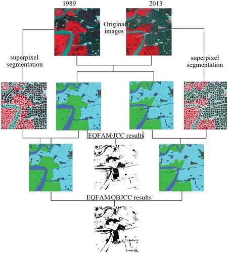
Figure 2 shows the EQFAM-JCC algorithm architecture.

Figure 2. Object-based entropy query-by fuzzy ARTMAP joint classification change detection diagram.

3. Data description and design of experiments

3.1 The description of the study area

Liaohe estuary wetland is situated in Liaoning province in the northeast China at latitude of 40°41′N to 41°27′N and the longitude of 121°34′E to 122°29′E as shown in Figure 3. Reed is the dominant plant in Liaohe estuarine wetland.

Figure 3. Study area in Liaohe estuarine wetland.

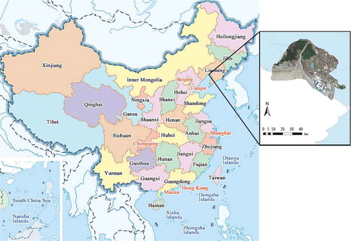
The reed wetlands contain a wide range of biodiversity and can act as crucial staging and breeding areas for migratory bird populations, including some globally threatened species. Thus, the wetland plays a critical role in ecological and environmental protection. Liaohe estuary delta is the leading economic center of Northeast China with an extensive industry based on the abundant oil and natural gas resources. With increasing intervention of these human activities, the reed wetland of Liaohe estuary is facing a constant threat of loss and degradation. More and more wetlands have been reclaimed because of the excessive population growth and the increasing demands for cultivable lands. The land reclamation for both agriculture and aquaculture is likely to affect the production, transport, and burial of Liaohe estuarine wetlands. These lead to estuary wetland land use/cover pattern changed seriously with ecosystem services.

All the images studied in this article have been pre-processed by geometric registration and radiation correction which are shown in Figure 4. Detailed information of 8-temporal remote sensing image is listed in Table 1.

Table 1. Detailed information of remote sensing images used in the experiments.

Year	Data	Satellite	Sensor
1987	21 September	Landsat 5	TM
1989	22 June	Landsat 5	TM
1995	11 September	Landsat 5	TM
2000	22 July	Landsat 5	TM
2004	19 August	Landsat 5	TM
2009	3 October	Landsat 5	TM
2013	23 May	Landsat 8	OLI
2014	26 May	Landsat 8	OLI

Figure 4. True color remote sensing images of the study area captured in 1987, 1989, 1995, 2000, 2004, 2009, 2013, and 2014.

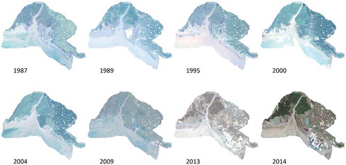
In order to explain the validity of the proposed method more clearly, two-temporal sub-study images with the size of 357 × 318 is acquired from the whole study area. One was clipped from 1989, and the other image was clipped from 2013. False color images of the sub-study area are shown in Figure 6.

Figure 5. Comparison of classification accuracy in 1989 remote sensing images with different number of initial training samples, (a) the initial number of training samples is 60, (b) the initial number of training samples is 70, (c) the initial number of training samples is 80, (d) the initial number of training samples is 90.

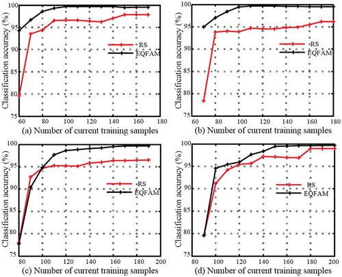
Figure 6. The process of pixel-based and object-based joint classification comparison in the sub-study area.

3.2 Design of experiments

To verify the feasibility and advantages of the proposed method in this article, simulation experiments are carried out on two-temporal remote sensing images in the sub-study area.

Firstly, the superiority of the proposed EQFAM classifier is verified. In this study, we first use the visual interpretation combined with the land use map to make a prior judgment of the land-cover types in the sub-study area. The land-cover types of the sub-study area are divided into four main categories (vegetation, paddy field, water body, building/road). The green, red, and near-infrared bands of the TM and OLI images were selected to construct the data sets. The ERDAS software is used to select two sets of candidate samples in the two-temporal images, respectively, with a total number of 6000. Sixty samples were randomly selected as the initial training sample set L, 1000 as the candidate sample set U, and 4000 for the test set, respectively. Ten candidate training samples will be added in each iteration.

Secondly, the verification of EQFAM-JCC algorithm is conducted according to Sections 2.2 and 2.3. The training samples used for the independent classification and joint classification are the same. Then the change detection experiment based on the EQFAM-OBJCC is carried out. Besides, it will be compared with the pixel-wise FAM neural network joint classification comparison (FAM-JCC), FAM PCC, and K-means JCC method without AL.

4. Experimental results and discussions

4.1 Results for entropy query-by fuzzy ARTMAP (EQFAM) classification

The classification results obtained from the EQFAM method and random sample (RS) selection are shown in Figure 5 (only considering the classification result of 1989 image as a special case) and each curve shows the classification accuracy with the increase of current training samples.

It can be seen from Figure 5 that the overall classification accuracy of the two methods is increasing with the increase of the training samples, no matter how many initial samples. The method in this article can achieve the classification accuracy above 99%, which is obviously higher than that of RS selection method. It shows the validity of the proposed EQFAM AL method.

4.2 Results for EQFAM-OBJCC algorithm

After selecting two groups of training samples with EQFAM classification method, 80% of them are randomly selected to form the training set and the remaining 20% are the testing set. The training and testing of classification accuracy are conducted on the samples of the two-phase images, respectively, and the parameters obtained from the adjustment of network are shown in Table 2.

Table 2. The parameters of the FAM neural network.

					k	pct
0.001	1.000	0.010	0.900	0.990	4	0.6

Then the change detection experiment is carried out. The threshold result obtained from similarity matrix by Ostu method is th = 0.2510. The change detection process of the proposed pixel-wise EQFAM-JCC and object-wise EQFAM-OBJCC is intuitively illustrated in Figure 6.

The classification results of remote sensing images obtained by the different classification methods are shown in Figure 7. The change detection results obtained by corresponding five methods are shown in Figure 8.

Figure 7. Comparison of classification result for different methods between 1989 and 2013 remote sensing images. (a) The original false color images, (b) FAM-PCC with average accuracy of 86.93%, (c) K-means-JCC with average accuracy of 88.89%, (d) FAM-JCC with average accuracy of 90.52%, (e) EQFAM-JCC with average accuracy of 91.98%, (f) EQFAM-OBJCC with average accuracy of 94.12%.

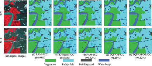
Figure 8. Comparison of change detection results for different methods between 1989 and 2013 remote sensing images. (a) FAM-PCC with total error of 39.38%, (b) K-means-JCC with total error of 37.78%, (c) FAM-JCC with total error of 32.04%, (d) EQAM-JCC with total error of 30.94%, “(e) EQFAM-JCC (f) EQFAM-OBJCC with total error of 27.03%.

It can be seen from the classification results of the five methods in Figure 7 that the joint classifier can classify the invariant information of two remote sensing images into the same class, in which class consistencies of three kinds of joint classification results in Figure 7(c)–(e) are superior to independent classification result of fuzzy ARTMAP in Figure 7(b); in addition, EQFAM-OBJCC in 7(f) has less “pepper and salt” problem compared with other methods.

Figure 8 is change detection result obtained by Figure 7. It can be seen from Figure 8(a) that the error accumulation caused by independent classification generates more false detection, but change detection results of joint classification in Figure 8(b)–(d) are more consistent with the real changes. Figure 8(e) shows the best result with the clear profile of the change parts and has the best visual perception, which is more beneficial to locate the real change information more precisely.

The classification results of K-means method are closely related to the selection of initial clustering centers, so it is usually unsatisfactory when the initial clustering centers are randomly selected. Therefore, the results shown in Figure 7(c) are time-consuming and are at great random. What’s more, K-means is an unsupervised classification method which cannot determine the class of the classification, so it needs to reallocate labels with the help of visual interpretation. It reduces the degree of automation of change detection. In addition, the joint classification method avoids the classification for all the pixels in the two-temporal remote sensing images, which then reduces the workload of classification algorithm greatly.

To quantify the classification results of the proposed change detection method, we randomly select 306 checkpoints referring to visual interpretation and land use map to calculate the change error matrix. The misdetection rate, false alarm rate, average accuracy, and Kappa coefficient are shown in Table 3. The best results obtainedby the proposed EQFAM-OBJCC are in bold.

Table 3. Comparison of change detection results of five different methods.

	Misdetection rate (%)	False alarm rate (%)	Total error (%)	Average accuracy (%)	Kappa coefficient
FAM-PCC	11.10	27.27	38.38	86.93	0.7043
K-means-JCC	18.89	18.89	37.78	88.89	0.7324
FAM-JCC	15.82	16.48	32.04	90.52	0.7725
EQAM-JCC	18.89	12.05	30.94	91.18	0.7826
EQFAM-OBJCC	15.75	11.28	27.03	94.12	0.8233

4.3 Results for monitoring the reclamation changes of Liaohe estuary wetland using time-series remote sensing images

The proposed EQFAM-OBJCC method is used to detect the changes on time-series images shown in Figure 4. The study area mainly covers seven categories according to visual interpretation and land use map: water, marsh, paddy, mud, building, project, and pond. The classification results are shown in Figure 9.

Figure 9. Land use/cover classification results of Liaohe estuarine wetland in 1987, 1989, 1995, 2000, 2004, 2009, 2013, and 2014.

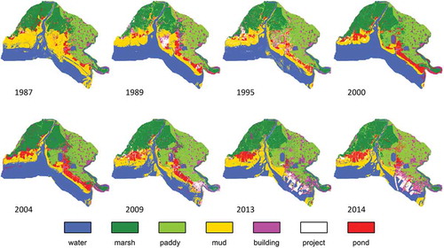
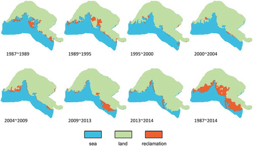
Classification results of remote sensing images are used to monitor the reclamation process. Each classification map is segmented into three parts: sea area, land area, and reclamation area. The reclamation monitoring results are shown as Figure 10. The increased reclamation area is marked with orange. The last sub-image of Figure 10 gives the reclamation change detection result between 1987 and 2014. Land area calculated using eight remote sensing images are listed in Table 4. From 1987 to 2014, this study area appeared continuously reclamation activity. Land area increased from 872.4654 to 1194.9372 km². The cumulative reclamation area reaches 364.3299 km².

Table 4. Statistical area of reclamation activity (km²) 1987–2014.

	1987	1989	1995	2000	2004	2009	2013	2014
Land area	872.465	936.515	1017.634	1035.392	1041.265	1091.336	1157.110	1194.937
Reclamation area	41.858	105.908	187.026	204.785	210.658	260.728	326.503	364.330

Figure 10. Reclamation monitoring results during 1987–1989, 1989–1995, 1995–2000, 2000–2004, 2004–2009, 2009–2013, 2013–2014, and 1987–2014.

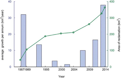
To reflect the intensity of reclamation process, average growth of land area per year were calculated and illustrated in Figure 11. During period from 1987 to 1989, average reclamation data showed a drastic activeness with the growth rate 32.025 km² per year. After that, from 1989 to 2000, as the end of the reclamation projects, the growth rate of reclamation slowed down to 3.5518 km² per year. The growth of the local population and influx of migrant workers made the coastal population increase dramatically, and expanded the demand for land and space. So a great upsurge in reclamation occurred after 2004. From May 2013 to May 2014, 37.8270 km² new land was observed by Landsat remote sensing image. And the reclamation project was still showing an active rising tendency. In Figure 11, it is more obvious that the reclamation process can be regarded as two different phases. From 1987 to 2000, this period includes the decrement phase of reclamation for sea aquaculture and farming industry, and the rising phase of reclamation for construction and project land is from 2000 to 2014.

Figure 11. Area change of reclamation from 1987 to 2014 (km²).

5. Conclusions

This article proposes an object-wise joint-classification change detection for remote sensing images based on entropy query-by fuzzy ARTMAP to counter the problems of error accumulation and “salt and pepper” effect caused by PCC. Firstly, this article proposes the entropy query-by fuzzy ARTMAP method to select the training samples with large amount of information for the neural network to improve the classification accuracy. Secondly, this article uses similarity thresholds to control the joint classifier to classify two-temporal remote sensing images simultaneously. Thirdly, the superpixels segmentation method is used to obtain the object-wise change detection result which reduces the “salt and pepper” effect. The experiment shows that this method reduces the error accumulation, the workload of classification algorithm, and the false detection rate to improve the precision of the change detection. Its change detection results are closer to the real changes which integrally improved the performance of the change detection. What’s more, the proposed method is used to monitor reclamation changes in Liaohe estuary wetland from 1987 to 2014.

Disclosure statement

No potential conflict of interest was reported by the authors.

Additional information

Funding

This work was supported by the project of the National Natural Science Foundation of China under grant number 61773087 and the Special Fund for Basic Research on Scientific Instruments of the National Natural Science Foundation of China under grant number 51327004.

References

- Achanta, R., A. Shaji, K. Smith, A. Lucchi, P. Fua, and S. Süsstrunk. 2012. “SLIC Superpixels Compared to State-Of-The-Art Superpixel Methods.” IEEE Transactions on Pattern Analysis and Machine Intelligence 34 (11): 2274–2282. doi:10.1109/TPAMI.2012.120.
- Berlanga-Robles, C. A., and A. Ruiz-Luna. 2011. “Integrating Remote Sensing Techniques, Geographical Information Systems (GIS), and Stochastic Models for Monitoring Land Use and Land Cover (LULC) Changes in the Northern Coastal Region of Nayarit, Mexico.” GIScience & Remote Sensing 48 (2): 245–263. doi:10.2747/1548-1603.48.2.245.
- Carpenter, G. A., S. Grossberg, N. Markuzon, J. H. Reynolds, and D. B. Rosen. 1992. “Fuzzy ARTMAP: A Neural Network Architecture for Incremental Supervised Learning of Analog Multidimensional Maps.” IEEE Transactions on Neural Networks 3 (5): 698–713. doi:10.1109/72.159059.
- Chang, N. B., M. Han, W. Yao, L. C. Chen, and S. Xu. 2010. “Change Detection of Land Use and Land Cover in an Urban Region with SPOT-5 Images and Partial Lanczos Extreme Learning Machine.” Journal of Applied Remote Sensing 4 (1): 043551–043551–15. doi:10.1117/1.3518096.
- Congalton, R. G., J. Gu, K. Yadav, P. Thenkabail, and M. Ozdogan. 2014. “Global Land Cover Mapping: A Review and Uncertainty Analysis.” Remote Sensing 6 (12): 12070–12093. doi:10.3390/rs61212070.
- Ghosh, A., B. N. Subudhi, and L. Bruzzone. 2013. “Integration of Gibbs Markov Random Field and Hopfield-Type Neural Networks for Unsupervised Change Detection in Remotely Sensed Multitemporal Images.” IEEE Transactions on Image Processing 22 (8): 3087–3096. doi:10.1109/TIP.2013.2259833.
- Gil-Sánchez, L., J. Garrigues, E. Garcia-Breijo, R. Grau, M. Aliño, D. Baigts, and J. M. Barat. 2015. “Artificial Neural Networks (Fuzzy ARTMAP) Analysis of the Data Obtained with an Electronic Tongue Applied to a Ham-Curing Process with Different Salt Formulations.” Applied Soft Computing 30: 421–429. doi:10.1016/j.asoc.2014.12.037.
- Hedjam, R., M. Kalacska, M. Mignotte, H. Z. Nafchi, and M. Cheriet. 2016. “Iterative Classifiers Combination Model for Change Detection in Remote Sensing Imagery.” IEEE Transactions on Geoscience and Remote Sensing 54 (12): 6997–7008. doi:10.1109/TGRS.2016.2593982.
- Hussain, E., and J. Shan. 2015. “Object-Based Urban Land Cover Classification Using Rule Inheritance over Very High-Resolution Multisensor and Multitemporal Data.” GIScience & Remote Sensing 53 (2): 1–19.
- Hussain, M., D. Chen, A. Cheng, H. Wei, and D. Stanley. 2013. “Change Detection from Remotely Sensed Images: From Pixel-Based to Object-Based Approaches.” ISPRS Journal of Photogrammetry and Remote Sensing 80: 91–106. doi:10.1016/j.isprsjprs.2013.03.006.
- Levinshtein, A., A. Stere, K. N. Kutulakos, D. J. Fleet, S. J. Dickinson, and K. Siddiqi. 2009. “Turbopixels: Fast Superpixels Using Geometric Flows.” IEEE Transactions on Pattern Analysis and Machine Intelligence 31 (12): 2290–2297. doi:10.1109/TPAMI.2009.96.
- Li, M., J. Im, and C. Beier. 2013. “Machine Learning Approaches for Forest Classification and Change Analysis Using Multi-Temporal Landsat TM Images over Huntington Wildlife Forest.” GIScience & Remote Sensing 50 (4): 361–384.
- Liu, M. Y., O. Tuzel, S. Ramalingam, and R. Chellappa. 2011. “Entropy Rate Superpixel Segmentation.” IEEE Conference on Computer Vision and Pattern Recognition (CVPR) 2097–2104.
- Lu, D., P. Mausel, E. Brondízio, and E. Moran. 2004. “Change Detection Techniques.” International Journal of Remote Sensing 25 (12): 2365–2401. doi:10.1080/0143116031000139863.
- Marchesi, S., F. Bovolo, and L. Bruzzone. 2010. “A Context-Sensitive Technique Robust to Registration Noise for Change Detection in VHR Multispectral Images.” IEEE Transactions on Image Processing 19 (7): 1877–1889. doi:10.1109/TIP.2010.2045070.
- Otsu, N. 1979. “A Threshold Selection Method from Gray-Level Histograms.” IEEE Transactions on Systems, Man, and Cybernetics 9 (1): 62–66. doi:10.1109/TSMC.1979.4310076.
- Otukei, J. R., and T. Blaschke. 2010. “Land Cover Change Assessment Using Decision Trees, Support Vector Machines and Maximum Likelihood Classification Algorithms.” International Journal of Applied Earth Observation and Geoinformation 12: S27–S31. doi:10.1016/j.jag.2009.11.002.
- Pal, M., A. E. Maxwell, and T. A. Warner. 2013. “Kernel-Based Extreme Learning Machine for Remote-Sensing Image Classification.” Remote Sensing Letters 4 (9): 853–862. doi:10.1080/2150704X.2013.805279.
- Peneva-Reed, E. 2014. “Understanding Land-Cover Change Dynamics of a Mangrove Ecosystem at the Village Level in Krabi Province, Thailand, Using Landsat Data.” GIScience & Remote Sensing 51 (4): 403–426. doi:10.1080/15481603.2014.936669.
- Shao, Y., and R. S. Lunetta. 2012. “Comparison of Support Vector Machine, Neural Network, and CART Algorithms for the Land-Cover Classification Using Limited Training Data Points.” ISPRS Journal of Photogrammetry and Remote Sensing 70: 78–87. doi:10.1016/j.isprsjprs.2012.04.001.
- Tuia, D., E. Pasolli, and W. J. Emery. 2011. “Using Active Learning to Adapt Remote Sensing Image Classifiers.” Remote Sensing of Environment 115 (9): 2232–2242. doi:10.1016/j.rse.2011.04.022.
- Voisin, A., V. A. Krylov, G. Moser, S. B. Serpico, and J. Zerubia. 2014. “Supervised Classification of Multisensor and Multiresolution Remote Sensing Images with a Hierarchical Copula-Based Approach.” IEEE Transactions on Geoscience and Remote Sensing 52 (6): 3346–3358. doi:10.1109/TGRS.2013.2272581.
- Wu, K., L. Wei, X. Wang, and R. Niu. 2016. “Adaptive Pixel Unmixing Based on a Fuzzy ARTMAP Neural Network with Selective Endmembers.” Soft Computing 20 (12): 4723–4732. doi:10.1007/s00500-015-1700-y.
- Ye, S., D. Chen, and J. Yu. 2016. “A Targeted Change-Detection Procedure by Combining Change Vector Analysis and Post-Classification Approach.” ISPRS Journal of Photogrammetry and Remote Sensing 114: 115–124. doi:10.1016/j.isprsjprs.2016.01.018.
- Zanotta, D. C., L. Bruzzone, F. Bovolo, and Y. E. Shimabukuro. 2015. “An Adaptive Semisupervised Approach to the Detection of User-Defined Recurrent Changes in Image Time Series.” IEEE Transactions on Geoscience and Remote Sensing 53 (7): 3707–3719. doi:10.1109/TGRS.2014.2381645.
- Zhang, C., Y. Chen, and D. Lu. 2015. “Detecting Fractional Land-Cover Change in Arid and Semiarid Urban Landscapes with Multitemporal Landsat Thematic Mapper Imagery.” GIScience & Remote Sensing 52 (6): 700–722. doi:10.1080/15481603.2015.1071965.
- Zhou, Y., J. Lian, and M. Han. 2016. “Remote Sensing Image Transfer Classification Based on Weighted Extreme Learning Machine.” IEEE Geoscience and Remote Sensing Letters 13 (10): 1405–1409. doi:10.1109/LGRS.2016.2568263.
- Zhu, Z., and C. E. Woodcock. 2014. “Continuous Change Detection and Classification of Land Cover Using All Available Landsat Data.” Remote Sensing of Environment 144: 152–171. doi:10.1016/j.rse.2014.01.011.