Effect of flying altitude and pulse repetition frequency on laser scanner penetration rate for digital elevation model generation in a tropical forest

Abstract

In tropical forests, the penetration ability of airborne laser scanning (ALS) may be limited because of highly dense vegetation cover. However, in the typical planning of ALS surveys, the ability of laser pulses to penetrate forests is not considered. Nine round-trip flight lines covering the area of a tropical forest on the northeast side of the Tsengwen Reservoir in Taiwan were designed in this study. Five flight lines flew at altitudes of 1.525, 1.830, 2.135, 2.440, and 2.745 km, and the other four had pulse repetition frequencies (PRFs) of 100, 150, 200, and 250 kHz. The laser penetration index (LPI) is a quantitative index measuring the penetration ability of the ALS and consists of the ratio of the number of laser pulses reaching the forest floor to the total number of laser pulses. The LPI was used to represent the laser penetration rate and investigate the influence of flying altitude and PRF on the LPI. The results showed that as the flying altitude decreased by 1 km, the average LPI increased by 10%, and as the PRF decreased by 50 kHz, the average LPI increased by 2%. The effect of the LPI on digital elevation models (DEMs) was confirmed by visual images obtained by DEMs at five altitudes. The DEM obtained at an altitude of 2.745 km was coarsely textured, whereas that obtained at an altitude of 1.525 km was finely textured. The in-situ height data obtained from the electronic Global Navigation Satellite System (eGNSS) were compared with the data of the ALS-generated DEMs. The results indicated that when the LPI ≥60%, the height difference between the in situ data and DEM data was not prominent. However, when the LPI <60%, the ALS-derived DEM could be higher or lower than the in-situ height; the largest difference between the two was 1.7 m. The LPI of a forest should be considered for ALS survey planning, especially when consistent DEM precision for large tropical forest areas is paramount.

Keywords:

• laser penetration index
• airborne laser scanning
• digital elevation model
• flying altitude
• pulse repetition frequency

1. Introduction

Airborne laser scanner (ALS) consists of a laser scanner, a Global Navigation Satellite System (GNSS), and an inertial measurement unit, and is used to obtain three-dimensional (3D) point cloud data (Shan and Toth 2008). When ALS is employed to scan a forest area, the laser pulse travels through the atmosphere and reaches the forest canopy. A certain amount of laser pulse energy is reflected back to the ALS receiver by leaf surfaces and branches and is recorded as a 3D point cloud (Heritage and Large 2009). If the remainder of the laser pulse energy continues downward, penetrating the vegetation layer, it can reach the forest floor layer and be reflected back to the ALS receiver. The laser echo signal that reflects from the bare surface of the forest floor is called the ground point (Maltamo 2014).

Because of its penetration ability, ALS has been used extensively to obtain digital elevation models (DEMs) of forests (Wang, Tseng, and Chu 2014; Chu et al. 2014). In tropical forest, however, the penetration ability of ALS may be limited because of highly dense vegetation cover. For example, in an ALS project conducted by the Central Geological Survey (CGS) of Taiwan to create a 1-meter resolution DEM for the island of Taiwan, the ground point density could not be maintained at a homogenous level over the whole island; ground point density is generally low in tropical forest areas compared with other areas in Taiwan. DEM data generated from a low ground point density are inadequate for identifying landscape scarps under a canopy (Chu et al. 2014). The four surveying companies in charge of the CGS project solved this problem through repeated scanning (i.e. flying over the same area two or three times). This solution was effective but time consuming; the number of ground points exhibited only marginal increments in hard-to-penetrate tropical forest after each scan.

Typically, ALS surveys consider flying altitude, pulse repetition frequency (PRF), laser beam divergence, field of view, trajectory position, and scan frequency to achieve the required point density. However, Chu et al. (2014) proposed that ALS surveys should be planned to maximize the ground point density in order to achieve better DEM quality. Theoretically, this could be achieved by incorporating the laser penetration ability of a forest into the design of an ALS survey by using a metric that quantifies laser penetration ability. However, ground point density and laser penetration ability are challenging issues for flight planning. These two factors depend not only on the sensor and flight characteristics, but also on the landscape characteristics. Similar to all other remote sensing detectors, an ALS receiver is limited by the signal-to-noise ratio. An ALS receiver cannot detect laser echo signals with overly weak energy, and thus cannot generate point data from those signals (Zhou et al. 2013; Su et al. 2016). Therefore, the amount of energy received by the ALS directly affects its forest penetration ability. According to previous studies, as the path length of a laser pulse increases, the effects of atmospheric absorption and spherical spreading loss increase, resulting in a reduction in the energy of laser echo signals (Morsdorf et al. 2008). In addition, many ALS systems exhibit increases in pulse energy with decreasing PRF (Chasmer et al. 2006; Morsdorf et al. 2008; Shan and Toth 2008). Laser penetration ability through a canopy depends on incident direction, often with a larger incident angle resulting in lower penetration ability (Zhao and Popescu 2009). In addition, decreasing the beam divergence increases the pulse energy (Andersen, Reutebuch, and McGaughey 2006; Hopkinson 2007). The density of the forest canopy layer also influences laser penetration ability; the lower the density of the forest canopy layer, the higher is the laser penetration ability (Pope and Treitz 2013; Wasser et al. 2013; Alonzo et al. 2015).

Laser penetration ability in a forest area can influence DEM quality, as can the parameters of a flight plan such as the flying altitude, PRF, beam divergence, and look angle (Morsdorf et al. 2008); environmental factors such as canopy condition (Morsdorf et al. 2008; Salleh, Ismail, and Rahman 2015) and slope (Salleh, Ismail, and Rahman 2015); and ground point density (Chu et al. 2014). In addition, DEM quality is influenced by the following aspects of ALS data processing: ground extraction methods (Pingel, Clarke, and McBride 2013; Maguya, Junttila, and Kauranne 2014; Kim and Eo 2015) and interpolation methods (Chu et al. 2014; Montealegre, Lamelas, and de la Riva 2015; Sterenczak et al. 2016).

The laser penetration index (LPI) is a quantitative index measuring the penetration ability of ALS (Hopkinson 2007; Morsdorf et al. 2008; Naesset 2009). Previous studies have proposed numerous LPI estimation formulas that can be categorized into point-based and intensity-based methods. The point-based methods comprise two estimation methods, one of which involves calculating the ratio of the number of ground points to the total number of ALS points (including multiple echoes) within a unit area (Takahashi et al. 2006; Hopkinson 2007; Zhao and Popescu 2009; Solberg 2010; Alonzo et al. 2015), and the other of which involves calculating the proportion of laser pulses that reach the forest floor, which is usually defined as the ratio of the number of laser pulses reaching the forest floor to the number of laser pulses within a unit area (Takahashi et al. 2006; Zhao and Popescu 2009; Peduzzi et al. 2012; Racine et al. 2014). The intensity-based method involves calculating the ratio of the total intensity of the ground points to the total intensity of the unit area (Hopkinson 2007; Zhao and Popescu 2009; Peduzzi et al. 2012). In this study, we selected a penetration index by calculating the ratio of the number of laser pulses reaching the forest floor to the number of transmitted laser pulses, which was advantageous because the number of transmitted laser pulses can be obtained during flight planning. Therefore, through this method, the number of laser pulses reaching the forest floor can be predicted.

Previous studies have reported that a sufficient number of ground points can generate DEMs of superior accuracy (Wang, Tseng, and Wang 2016) that can be used to support various applications such as forest structure determination (Clark, Clark, and Roberts 2004; Chasmer et al. 2006; Naesset 2009), forest biomass estimation (Baltsavias 1999; Zhao, Popescu, and Nelson 2009; Naesset 2011; Singh et al. 2015), and landscape scarp identification (Chu et al. 2014). The number of ground points of an ALS survey can be increased by increasing the laser pulse density with multiple flight lines or by increasing the laser penetration ability by manipulating the flying altitude and PRF of the ALS. However, increasing the laser pulse density increases the flight cost (Hummel et al. 2011; Zhao et al. 2016) and renders the already massive data volume even larger and more difficult to process. In addition, in mountainous tropical rainforest areas in Taiwan, using repeated flight lines to increase the laser pulse density consumes the scarcely available cloud-free time. By contrast, increasing the LPI value by manipulating the flying altitude and PRF (Chasmer et al. 2006; Morsdorf et al. 2008) puts the cloud-free time to good use. Notably, increasing the PRF introduces greater ranging ambiguity (Rieger 2014), and a lower flying altitude denotes lower coverage and more flight lines.

Considering the permitted budget and the priorities of the factors in ALS flight plans, a mountainous area with apparent topographical features and a dense tropical forest area were selected to explore the following three issues: (1) the influences of flying altitude and PRF on the LPI value, (2) changes in the LPI values of various types of vegetation under various flying altitudes, and (3) the influence of LPI on the production of DEMs and the comparison between errors and visual differences.

2. Study area and data

2.1. Study area

The study area was located on the northeast side of the Tsengwen Reservoir (23° 18ʹ N, 120° 39ʹ E) in Tainan City, Taiwan. The altitude of the study area ranged between 230 and 850 m and comprised low-altitude tropical evergreen broadleaf forests, as shown in Figure 1(a). The photo locations are indicated by the text in black in Figure 1(b). The study area encompassed two forest types, namely mixed forest and bamboo forest, and an areca orchard type (Areca catechu Linn). Specifically, the mixed forest included Taiwan acacia (Acacia confusa Merr), large-leaved nanmu (Machilus kusanoi Hayata), red cedar (Bischofia javanica Blume), and turn-in-the-wind (Mallotus paniculatus Lamm). The bamboo forest contained thorny bamboo (Bambusa stenostachya Hackel), makino bamboo (Phyllostachys makinoi Hayata), and Taiwanese giant bamboo (Dendrocalamus latiflorus Munro). The three types of vegetation (mixed forest, bamboo forest, and areca orchards) were selected for this study because they have clearly distinguishable features and cover large areas. Considering the three types of vegetation and their canopy density, on 10 July 2014, we used an LAI-2000 plant canopy analyzer to measure the leaf area index (LAI) at a distance of 1 km from the sample area. The average LAI of the mixed forest was 4.43 (n = 3), that of the bamboo forest was 3.84 (n = 2), and that of the areca orchards was 2.31 (n = 1). The time interval between the LAI measurement and ALS survey was approximately 1 year.

Figure 1. The study area from which the ALS dataset was produced was located at the Tsengwen Reservoir in Tainan City, Taiwan. (a) In situ photos of three different tree species in the study area. Site A: mixed forest and canopy of mixed forest; Site B: bamboo forest; Site C: Areca orchard. The photo locations are marked in Figure 1(b). (b) Spatial distribution of mixed forest, bamboo forest, and areca orchard. (c) ALS swathes with five flying altitudes (black lines) and four PRFs (blue lines). The area of flying altitudes where the swathes overlap is that represented by the slashed black line. The area of PRFs where the swathes overlap is that represented by the sky blue polygon. The red rectangle denotes the subset area shown in Figure 13. (d) The 38 red dots denote in-situ eGNSS measurements. For full colour versions of the figures in this paper, please see the online version

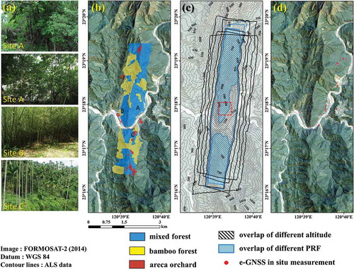
The spatial distribution of these three types of vegetation was identified through manual digitalization by using the aerial photos (20 cm pixel resolution) obtained at the same time as the ALS data (Figure 1(b)). Three professional employees examined and categorized the three types of vegetation multiple times, and all the types could be clearly identified in the aerial photos. The digitalization results were not assessed analytically; however, they were confirmed by field investigation to have high fidelity. Because the ALS survey was conducted from 07:17 to 10:23 in the morning, there were varying shadows caused by the mountainous terrain. Although this had minimal effect on the manual task of identifying the vegetation types, the resultant mosaic orthophoto was not visually pleasing as a whole. For this cosmetic reason, a FORMOSAT-2 satellite image acquired in 2014, which has been pan-sharpened to 2 m resolution and enhanced by the ALS DEM hillshades, was used as the background images shown in Figure 1(b) and Figure 1(d). No prominent change of the landscape was found between the 2013 orthophoto and the 2014 FORMOSAT-2 image, as there were no severe events that occurred between 2013 and 2014 at the study site.

2.2. ALS dataset

The ALS dataset was acquired using an Optech PEGASUS HD400 system on 25 July 2013. The HD400 ALS operates at a wavelength of 1064 nm and has a beam divergence of 0.25 mrad. Nine round-trip flight lines covering the tropical forest on the northeast side of the Tsengwen Reservoir, Taiwan, were designed in this study. Five of the flight lines flew at different flying altitudes and the other four had different PRFs.

To investigate the influence of flying altitude on the LPI of the tropical forest in our study area, five flight lines were designed for scanning with flying altitudes of 2.745, 2.440, 2.135, 1.830, and 1.525 km above sea level (ASL). ALS was performed through back and forth flying (Table 1). The other flight parameters for the five flight lines were identical; for example, the PRF was 100 kHz, the scanning angle was ± 20°, and the scanning frequency was 40 Hz. Therefore, the resultant laser pulse densities obtained using the various flying altitudes were all between 0.7 and 1.5 pulses/m². The swathes corresponding to the five flight lines also varied, as indicated by the black lines in Figure 1(c). This study focused on the overlapping area of the five flight lines (i.e. the black slash area in Figure 1(c)).

Table 1. Summary of ALS dataset.

Flight Heading (deg.)	PRF (kHz)	Flying Alt. (ASL km)	Laser Pulse Density (pulses/m^2)
185	100	1.525	1.5
5.8	100	1.830	1.2
185	100	2.135	1.0
5.8	100	2.440	0.9
185	100	2.745	0.7
5.8	100	1.403	1.5
185	150	1.403	2.2
5.8	200	1.403	3.0
185	250	1.403	4.1

Scan Frequency: 40 Hz; eye-safety enabled.

To investigate the influence of PRF on the LPI, four flight lines were designed for ALS with PRFs of 100, 150, 200, and 250 kHz. ALS was performed through back and forth flying (Table 1). The other flight parameters for these four flight lines were identical; for example, the flying altitude was 1.403 km; the scanning angle was ± 20°; and the scanning frequency was 40 Hz. The resultant laser pulse densities obtained using the four PRFs ranged between 1.5 and 4.1 pulses/m². The four swathes had identical widths because the four flight lines all had the same flying altitude and field of view (as indicated by the blue lines in Figure 1(c)). However, because the maximum measurable range for the PRF of 250 kHz must be lower than 0.8 km above ground level (AGL), and because the relatively low-lying area of the river valley in the study area was higher than 0.8 km AGL, no ALS data were obtained for this area, as shown in Figure 1(c). This study focused only on the overlapping area of the four swathes with different PRFs (i.e. the sky blue area in Figure 1(c)).

2.3. In situ height measurement of bare ground in the forest

To investigate the relationship between the accuracy of the ALS-derived DEMs and the LPI, this study used a Trimble 5700 electronic GNSS (eGNSS) receiver to measure the height of the bare forest ground within the study area. The root-mean-square error (RMSE) values of the vertical and horizontal measurements were 0.02 and 0.01 m ± 1 ppm, respectively, and were measured via a network (e.g. Groupe Speciale Mobile (GSM)) connection to the virtual reference station provided by the National Land Surveying and Mapping Center, Taiwan, when the fixed solution was available in the forest. The accuracy of the eGNSS was comparable to that in reports from other dense forest areas (Pirti 2008; Naesset et al. 2000). Because of accessibility in the field, a total of 38 height values were obtained, all of which were ca. 10–20 m away from roads (Figure 1(d)). Because the overlapping area for PRF comparison (i.e. the sky blue area in Figure 1(c)) was far from any roads, in-situ height measurements were not conducted in this area.

A total of 38 eGNSS measurements were obtained (i.e. the red dots in Figure 1(d)) within the ALS survey area. The five flight lines had different swath widths; the flying altitude of 1.525 km had the smallest swath width, whereas that of 2.745 km had the largest swath width. Therefore, the swathes of the flying altitudes from 1.525 to 2.745 km separately encompassed 14, 19, 24, 33, and 38 eGNSS points.

3. Methodology

3.1. LPI

To link the results of our study to ALS survey planning for DEM generation, where meeting the requirement of laser pulse density and estimating the number of ground points are critical, the LPI was calculated as follows:

(1)

where denotes the number of laser pulses that reached the forest floor layer in a unit area and denotes the number of transmitted laser pulses in a unit area. In this study, we used a 10 m × 10 m grid as the unit area.

To accurately calculate the value of in the ALS data, we considered that every single transmitted laser pulse has a unique GNSS time and that the multiple echoes that were generated along with each laser pulse would share the same GNSS time. Therefore, the value of can be obtained by calculating the number of transmitted laser pulses at various GNSS times in a unit area. In the preprocessing step, the high and low points of the ALS data are filtered out, which makes the number of first or last echoes less than the number of transmitted laser pulses (). Clouds, birds, and high-voltage cables in the natural environment yield points that are significantly higher than other points in ALS data (Anderson and Pitlick 2014), and these points need to be filtered out. In contrast, in a forest region, the last echo in the ALS data may be the low point because of the multipathing phenomenon, which causes the ALS data to appear below ground (Gatziolis and Andersen 2008).

The number of laser pulses that reached the forest floor layer () in this study was estimated as follows. The ground points of each flight line were extracted using an automatic classification routine (Soininen 2000) implemented in TerraScan software followed by manual modification for the areas where the automatic classification results were less optimal. This manual modification was crucial because it helped improve the DEM quality sufficiently to meet the requirements of our local users. A DEM for each flight line was then generated from the ground points by using the triangulated irregular network (TIN) interpolation method. An elevation threshold value of 2 m above the DEM was used to identify the ALS points of the forest floor layer (Riano et al. 2004; Morsdorf et al. 2006; Morsdorf et al. 2008). ALS points below this threshold were regarded as points within the forest floor layer. Because a single laser pulse may generate more than one point within the forest floor layer (i.e. grasses and shrubs), the calculation of followed the same procedure as that of , which used the GNSS time stamp to avoid repeated calculation of the number of points in the forest floor layer.

3.2. Data analysis

In this study, in order to explore the influences of flying altitude and PRF on the LPI value, ALS data produced by the flights with five different flying altitudes and four different PRFs were used to calculate the LPI values based on the size of a unit area (a 10 m × 10 m grid). In addition, the lowest laser pulse density in this ALS data was 0.7 pulse/m², and each LPI grid had an average of at least 70 laser pulses for calculation. Furthermore, the area with a penetration rate of 1 was removed. This area contained buildings, valleys, roads, and open spaces and was not a forest area. Regarding statistical charts, in this study, histograms and box plots were used to present various LPI values for the various flying altitudes, PRFs, and types of vegetation. A histogram was used to present a frequency distribution, and a box plot was used to present the average, median, and lower and upper quartiles.

In this study, the elevation difference and RMSE were used to assess the ALS-derived DEM accuracy. The elevation difference was expressed as follows:

(2)

where the height measured using eGNSS measurement was denoted as and the height of the ALS-derived DEM obtained from each of the various flying altitudes was (where h denotes the flying altitudes, which were 1.525, 1.830, 2.135, 2.440, and 2.745 km). The ALS-derived DEM was obtained according to the TIN data composed of ground points; the DEM contained 1 m grid. And, was extracted from the ALS-derived DEM pixel in the same position as .

For each in situ location, the LPI value could also be extracted for different flying altitudes. To understand the relationship between the LPI and RMSE, a LPI interval of 0.2 was adopted. And, RMSE was expressed as follows:

(3)

where denotes the total number of measurement pairs between the ALS-derived DEM and the eGNSS-measured height for each LPI interval.

3.3. Point cloud resampling

It has been reported that DEM accuracy is also affected by laser pulse density, i.e. high laser pulse density results in high DEM accuracy (Chu et al. 2014). However, the current study constituted a rare case in which we could obtain datasets from different flying altitudes while using the same laser pulse density. Thus, we randomly resampled the ALS data of the four lower flying altitudes (i.e. 1.525, 1.830, 2.135, and 2.440 km) so that they had the same laser pulse density (i.e. ca. 0.65 pulses/m²) as that of the highest flying altitude (i.e. 2.745 km) for a subset area of 300 m × 300 m (denoted as the red rectangle in Figure 1(c)). By doing so, the effect of laser pulse density on the quality of the ALS-derived DEMs, which were produced by TIN, should have been minimized.

4. Results

4.1. LPI at different flying altitudes

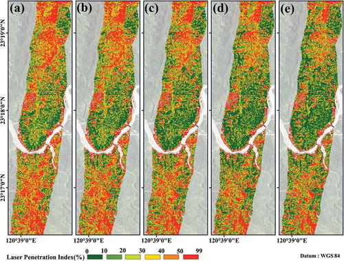
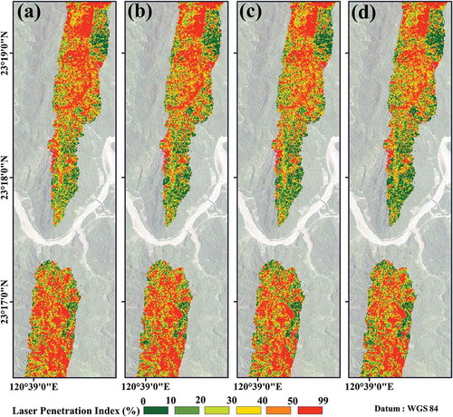
This study investigated the influence of five flying altitudes on the LPI in a tropical forest. The difference between each flying altitude was 0.3 km. In the area where the LPI <1, the overlapping area of the five flying altitudes was 5.07 km². Figure 2(a)–(e) show the LPI results; red and green represent high and low LPI values.

Figure 2. LPIs of different flying altitudes. (a) 1.525 km; (b) 1.830 km; (c) 2.135 km; (d) 2.440 km; (e) 2.745 km.

To reveal the of change in LPI resulting from the change in flying altitude, the LPI difference maps of two neighboring flying altitudes (e.g. 1.525 and 1.830 km) were computed and are shown in Figure 3(a)–(d), where the LPI from the lower flying altitude was subtracted from that of the higher flying altitude for each 10 m × 10 m grid. It is obvious that a large portion of the region has positive LPI difference values when the flying altitude was decreased. However, an interesting pattern of the regions with negative LPI differences was found to be likely present in the northern part of the study area (denoted as region A in Figure 3(a) and (c)) when the lower flying altitudes were 1.525 km and 2.135 km, respectively, and the flight heading was 185 degree (Table 1). When the flight heading of the lower flying altitude was 5.8 degrees (Table 1), which had the flying altitudes of 1.830 km and 2.440 km, respectively, the regions with negative LPI differences seemed likely to be present in the southern part of the study area (denoted as region B in Figure 3(b) and (d)).

Figure 3. LPI difference maps. (a) – (d) Opposite flight heading, where (a) 1.525 km vs. 1.830 km, (b) 1.830 km vs. 2.135 km, (c) 2.135 km vs. 2.440 km, and (d) 2.440 km vs. 2.745 km. (e) – (g) Same flight heading, where (e) 1.525 km vs. 2.135 km, (f) 1.830 km vs. 2.440 km, and (g) 2.135 km vs. 2.745 km. The arrow in (g) denotes the profiles shown in Figure 4.

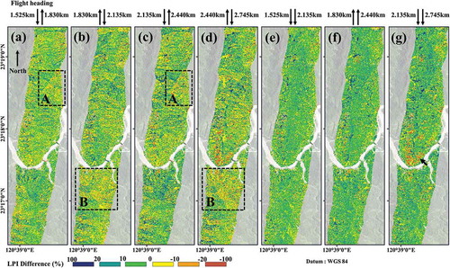
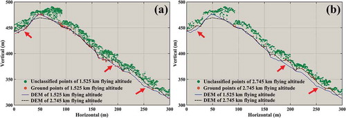
Figure 4. Point cloud and DEM profiles. (a) 1.525km; (b) 2.745 km.

A further investigation was conducted by computing the LPI difference maps for two flight lines with different flying attitudes but having the same heading and PRF setting. The results are shown in Figure 3(e)–(g), respectively, for the paired flying altitudes of 1.525 km versus 2.135 km and 2.135 km versus 2.745 km for the flight heading of 185 degrees and 1.830 km versus 2.440 km for the flight heading of 5.8 degrees. It is obvious that the majority of the study area showed positive LPI difference values while the negative LPI difference values took up only a small fraction of the overall study area and were scattered.

A rather persistent region with negative LPI difference values is denoted by an arrow in Figure 3(g). It was found that the negative LPI difference values were actually associated with the DEM derived from the point clouds of each different flying altitude. Figure 4(a) and (b) show the profiles, with a width of 5 m, of the point clouds from the flying altitudes of 1.525 km and 2.745 km, respectively, for this region. In this study, because the ground points were classified and followed by DEM generation for each flying altitude independently, the DEMs shown in Figure 4(a) and (b) are not exactly the same, although the general topographic features are similar. Three particular locations (denoted by the arrows in Figure 4) revealed the exemplary case that the DEM from the higher flying altitude of 2.745 km was higher than that of the lower flying altitude of 1.525 km due to poor laser penetration ability. In the process of determining the number of laser pulses that reached the forest floor layer, a higher DEM would include more points above it when an elevation threshold value is considered (in this case, a value of 2 m was used). As a result, a high LPI value was produced for a flying altitude with poor laser penetration ability. Fortunately, such biases were less prominent in the flying altitudes lower than 2.745 km.

The LPI values obtained using the various flying altitudes are displayed as the histograms and box plots shown in Figure 5(a) and (b), respectively. As shown in Figure 5(a), when the LPI >20%, all the flying altitudes had similar histogram values; when the LPI <20%, the flying altitudes had different values. The smallest LPI value increased substantially from 2% to 12% when the flying altitude was reduced from 2.745 to 1.525 km. In an ALS survey, reducing the proportion of areas with the smallest LPI is crucial because the ground points in these areas (with the minimum LPI value) are typically sparse; therefore, the DEM values in these areas are likely to be estimated using the ground points of the surrounding area through the interpolation method. Thus, if the overall area with a low LPI can be further reduced, the quality of the ALS-derived DEM can be considerably improved.

Figure 5. Histograms and box plots of different flying altitudes. (a) histograms. (b) box plots. The dots and squares in (b) denote the average and median LPI values, respectively.

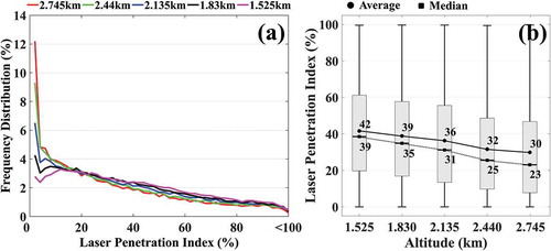
According to Figure 5(b), the lower and upper quartiles of the LPI increased as the flying altitude decreased. In particular, the average LPI values were 30% and 42% when the flying altitudes were 2.745 km and 1.525 km, respectively, which means that the average LPI value increased by 12% when the flying altitude was decreased by 1.22 km. Similarly, the median LPI values were 23% and 39% when the flying altitudes were 2.745 km and 1.525 km, respectively, which means that the median LPI value increased by 16% when the flying altitude was decreased by 1.22 km. Roughly speaking, for this study area, the average and median LPI values increased by 10% and 13%, respectively, when the flying altitude was decreased by 1 km.

The above results suggested that decreasing the flying altitude led to an increase in the LPI and that the heading of the flight lines also contributed to the change in the LPI.

4.2. LPI at different PRFs

In this study, we further tested the influence of four PRFs (i.e. 100, 150, 200, and 250 kHz) on the LPI. The overlapping area of the four PRFs was ca. 3.56 km², as displayed in Figure 6(a)–(d). The overall visual appearance of Figure 6(a)–(d) is highly similar in all parts.

Figure 6. LPIs of different PRFs. (a) 100kHz; (b) 150kHz; (c) 200kHz; (d) 250kHz.

To emphasize the increase in the LPI with decreasing PRF, the LPI difference maps of two neighboring PRF settings (e.g. 100 and 150 kHZ) were computed and are shown in Figure 7(a)–(c), where the LPI from the lower PRF was subtracted from that of the higher PRF for each 10 m × 10 m grid. It is obvious that most of the region showed positive LPI difference values when the PRF was decreased. However, an interesting pattern of the regions with negative LPI differences was found to be likely present in the southern part of the study area (denoted as region A in Figure 7 (a) and (c)) when the lower PRFs were 100 kHz and 200 kHz, respectively, and the flight heading was 185 degrees (Table 1).

Figure 7. LPI difference maps. (a) – (c) Opposite flight heading, where (a) 100 kHz vs. 150 kHz, (b) 150 kHz vs. 200 kHz, and (c) 200 kHz vs. 250 kHz. (d) – (e) Same flight heading, where (d) 100 kHz vs. 200 kHz, and (e) 150 kHz vs. 250 kHz.

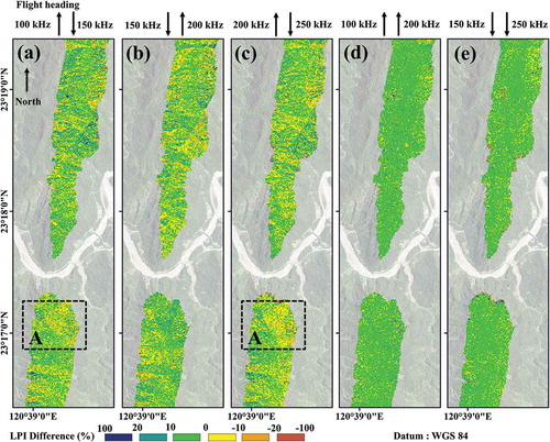
A further investigation was conducted by computing the LPI difference maps for two flight lines with different PRF settings but having the same flying altitude and heading. The results are shown in Figure 7(d) and (e), respectively, for the paired PRF settings of 100 kHz versus 200 kHz for the flight heading of 185 degrees and 150 kHz versus 250 kHz for the flight heading of 5.8 degrees. It is obvious that the majority of study area showed positive LPI difference values.

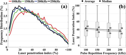
The LPI values obtained using the various PRFs are displayed as the histograms and box plots shown in Figure 8(a) and (b). According to Figure 8(a), all the PRFs had similar histogram trends; no clear differences were observed. According to Figure 8(b), the lower and upper quartiles of the LPI increased as the PRF decreased. In particular, the average LPI values were 44% and 38% when the PRFs were 100 kHz and 250 kHz, respectively, which means that the average LPI increased by 6% when the PRF was decreased by 150 kHz. Similarly, the median LPI values were 41% and 35% when the PRFs were 100 kHz and 250 kHz, respectively, which means that the median LPI increased by 6% when the PRF was decreased by 150 kHz. Roughly speaking, for this study area, the average and median LPI values both increased by 2% when the PRF was decreased by 50 kHz.

Figure 8. Histograms and box plots of different PRFs. (a) histograms. (b) box plots. The dots and squares in (b) denote the average and median LPI values, respectively.

4.3. LPIs of three different types of vegetation

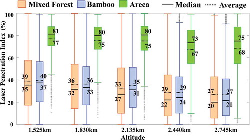
The area covered by the datasets obtained from the various flying altitudes (Section 2.1) contains three types of vegetation, namely, areca orchards, bamboo forest, and mixed forest. The vegetation distribution is shown in Figure 1(b). The relationship between the LPI of each type of vegetation and the flying altitude is illustrated in Figure 9. For all the flying altitudes, the LPI for the areca orchard areas (median = 75–81%; average = 68–77%) was larger than those for the bamboo forest (median = 27–40%; average = 21–37%) and mixed forest (median = 27–39%; average = 20–35%) areas. Notably, the medians and average LPI values varied among the three types of vegetation (areca orchards < bamboo forest < mixed forest), indicating that the penetration rate was also influenced by the type of vegetation. In addition, the LPI of the areca orchards remained almost the same when the flying altitude was low (1.525–2.135 km) but began to change when the flying altitude was 2.440 km or higher. This indicates that the LPI for the areca orchards was not substantially influenced by the changes in flying altitude. By contrast, the LPIs for the mixed forest and bamboo forest were heavily influenced to a similar extent by the flying altitude. Specifically, when the altitude was decreased from 2.745 to 1.525 km, the average LPIs increased by 15% (mixed forest) and 16% (bamboo forest). In addition, the median and average LPIs for the mixed forest and bamboo forest differed by only 4–1% at each respective flying altitude. These results indicate that, despite the drastic differences in the appearances of the two vegetation types (cf., Figure 1(a)), the mixed forest and bamboo forest exhibited the same relationship between flying altitude and the LPI.

Figure 9. LPI box plots of mixed forest, bamboo forest, and areca orchards for various flying altitudes.

4.4. Accuracy of ALS-derived DEM with different LPIs

Figure 10 shows the values of and the corresponding LPI values. Considering that the height accuracy of ALS is ± 0.15 m (ALS signals with a time resolution of 1 ns) (Pereira and Janssen 1999; Reutebuch et al. 2003; Sackov and Kardos 2014; Ivan et al. 2016) and that the published vertical accuracy of eGNSS is ± 0.02 m (Trimble 2003), if the value of was within ± 0.17 m (as denoted by the gray area in Figure 10), then and were regarded as identical. To further understand the data trend, the values of were divided into positive and negative clusters and the trend lines of each cluster were calculated using the moving average method with an LPI window size of ± 0.05 and an LPI overlap of 0.025. The positive and negative trend lines are denoted as and , respectively.

Figure 10. Scatter plot for and the corresponding LPIs of different flying altitudes.

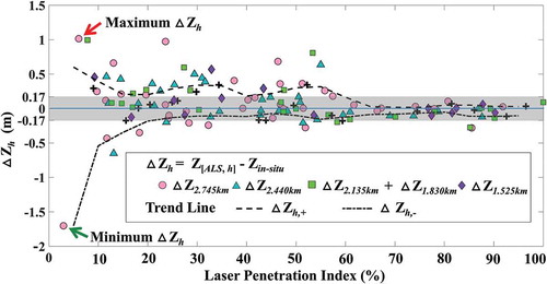
According to Figure 10, when the LPI ≥60%, most of the values were within ± 0.17 m; therefore, and were regarded as identical. Moreover, the values indicated that when the LPI < 60%, decreased with increasing LPI. Furthermore, the values in Figure 10 indicate that when the LPI was between 20% and 60%, no clear difference was observed among the values of . When the LPI <20%, decreased as the LPI increased.

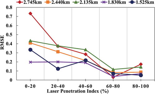
Figure 11 presents the results regarding the relationship between the LPI and RMSE. The RMSE value increased with the flying altitude, indicating that the flying altitude influenced the RMSE value. In addition, as the LPI value increased, the RMSE value decreased; when LPI ≥60%, the RMSE value was approximately 0.1, indicating that the errors between the ALS-derived DEMs and eGNSS-measured heights were reduced when LPI ≥60%.

Figure 11. Relationship between the LPI and RMSE at various flying altitudes.

Theoretically, when ALS has insufficient penetration ability in the forest, the DEM elevation is expected to be higher than the in situ height, which would lead to a result of . However, our results showed a negative . Therefore, to understand what yielded the maximum and minimum values of , the method of examining the profile was adopted to explore how extreme errors were caused. Accordingly, we examined the maximum (positive) and minimum (negative) values of , which are denoted by the red ( = 1.01 m; LPI = 6%) and green ( = −1.7 m; LPI = 2%) arrows in Figure 10, respectively.

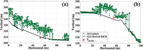
The profiles of the point clouds (thickness = 10 m) for the maximum (red arrow in Figure 10) and minimum (green arrow in Figure 10) are displayed, respectively, in Figure 12(a) and Figure 12(b), each of which represents a different forest area. The DEMs (black lines in Figure 12) of these areas were the outcomes of TIN interpolation of the neighboring ALS ground points. The red triangles indicate the in situ data. No ground points were observed when the X-axis values were between 22 and 58 m in Figure 12(a) and between 35 and 80 m in Figure 12(b). Because no ground points that were effectively penetrated by ALS existed around the in-situ positions, the DEM elevations and those obtained from the in situ measurements differed. The DEM values in such regions are the result of TIN interpolation based on neighboring ground points. As illustrated by Figure 12(b), the negative is attributed to the hilly terrain of the study site, where the low penetration area is surrounded by lower grounds.

Figure 12. Point cloud profiles with maximum and minimum . (a) maximum ; (b) minimum .

4.5. Impact of flying altitude on multiple returns

We selected a small area of mixed forest, denoted as the red dashed square in Figure 1(c), for which we randomly resampled the ALS data of the four lower flying altitudes so that they had the same laser pulse density as that of the highest flying altitude. Table 2 summarizes the number of multiple echoes (i.e. first, second, third, and fourth) and ground points for this small area. Overall, the numbers of first echoes were similar (maximum and minimum values: 87,917 and 86,230 points, respectively) for the flying altitudes between 1.525 and 2.745 km. The numbers of second, third, and fourth echoes increased as the flying altitude decreased, as did the number of ground points, which was approximately twice as high at a flying altitude of 1.525 km than at 2.745 km.

Table 2. Summary of ALS data in the small area denoted by the red dashed square in Figure 1(c).

Flying Altitude (km)	1.525	1.830	2.135	2.440	2.745
Number of Points
1st Echo	86,230	86,673	86,466	87,917	87,454
2nd Echo	54,294	50,166	45,614	40,285	31,906
3rd Echo	22,833	18,509	14,345	9668	4769
4th Echo	6548	4407	2731	1234	280
Ground Points	16,213	15,304	11,430	11,065	8707
Frequency Distribution (%)
1st Echo	50.7	54.2	58.0	63.2	70.3
2nd Echo	32.0	31.4	30.6	29.0	25.7
3rd Echo	13.4	11.6	9.6	6.9	3.8
4th Echo	3.9	2.8	1.8	0.9	0.2
Laser Pulse Density (pulse/m^2)	0.64	0.64	0.64	0.65	0.65

In accordance with the commonly used protocol, which analyzes multiple ALS echoes through frequency distribution, the number of first to fourth echoes was divided by the total number of point data for each flying altitude (Gobakken and Naesset 2008; Naesset 2009). The results are shown in Table 2 and indicate a trend of the first echo frequency decreasing with the flying altitude; the first echo frequency decreased from 70.3% at a flying altitude of 2.745 km to 50.7% at 1.525 km. In addition, the second, third, and fourth echo frequencies all increased when the flying altitude decreased, rising from 25.7%, 3.8%, and 0.2% at 2.745 km to 32.0%, 13.4%, and 3.9% at 1.525 km, respectively. This indicates that a lower flying altitude would increase the penetration ability in the forest, which correlates with the findings in our study using the LPI. Notably, the frequency distribution analysis was smoothly conducted for the ALS data after the data had been collected. However, frequency distribution analysis is unsuitable for the design of ALS survey planning because the number of points for each echo cannot be predicted before the ALS survey is conducted.

4.6. DEM quality in relation to five flying altitudes

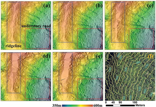
We selected a small area of mixed forest, denoted as the red dashed square in Figure 1(c), containing a ridgeline and understory road network. Figure 13 shows the ALS-derived DEMs of the randomly resampled data from the four lower flying altitudes and the intact data from the highest flying altitude. The understory road network, represented by the dashed red rectangle in Figure 13, was easily identifiable in the ALS-derived DEMs from the flying altitudes of 1.525, 1.830, and 2.135 km (Figure 13(a)–(c)), but less evident at the higher flying altitudes of 2.440 and 2.745 km (Figure 13(d)–(e)). The blue dashed rectangle in Figure 13 represents the ridgeline area, which changed dramatically from being finely textured where the ridgeline is prominently visible in Figure 13(a) at the flying altitude of 1.525 km, to coarsely textured as the flying altitude increased where the ridgeline is flattened in Figure 13(e) at 2.745 km. Judging from this change in DEM texture, the coarsely textured DEM was concluded to be of lower quality (Kraus et al. 2006).

Figure 13. DEMs developed from data obtained at various flying altitudes: (a) 1.525 km; (b) 1.830 km; (c) 2.135 km; (d) 2.440 km; (e) 2.745 km. (f) Orthophoto overlaid with elevation contours, derived from the original DEM of the flying altitude of 1.525 km.

5. Discussion

Based on our findings that the penetration ability of ALS is affected by flying altitude, PRF, vegetation type, and flight heading, it is recommended that these factors be taken into account when planning future flights for ALS.

With regard to obtaining LPI data, it has been reported that LPI values are highly correlated with vegetation indexes (i.e. NDVI, ratio vegetation index (RVI), perpendicular vegetation index (PVI), and soil-adjusted vegetation index (SAVI)) (Lee et al. 2015), which can be easily derived from satellite imagery with different resolutions provided by various sources. Information regarding the spatial distribution of vegetation types can be obtained either from classifying the relevant satellite images or from forestry agencies.

In considering the accuracy of DEMs obtained from an ALS survey, our results (Figures 10 and 11) indicated that high DEM accuracy could be obtained when the LPI was greater than 60%, while poor DEM accuracy was associated with lower LPI values. When the LPI value was lower than 20%, the DEM accuracy became worse. So, when designing an ALS flight plan, it is suggested that the flying altitude or PRF should be lowered when the vegetation indexes indicate a poor LPI value (Lee et al. 2015). In addition, some vegetation types (i.e. mixed forest and bamboo forest) may require lower flying altitudes or PRFs for better penetration.

As for the effect of flight heading on the laser penetration ability of ALS, our results did not provide enough information to make any conclusive suggestions because only two flight headings (i.e. 5.8 degrees and 185 degrees) were used. However, in light of the distinct patterns shown in the LPI difference maps from flight lines with the same flight heading (i.e. Figure 3(e)–(g), Figure 7(d) and (e)) and flight lines with opposite flight headings (i.e. Figure 3(a)–(d), Figure 7(a)–(c)), the effect of flight heading is a subject that deserves a more comprehensive investigation in the future.

Some shortcomings can be induced with lower flying altitudes and PRFs. For example, a rugged terrain may pose a threat to airborne operations if the flying altitude is too close to the terrain. In our experience, a helicopter can achieve a lower safe flying altitude than a fixed wing vehicle, at the price of a higher airborne operating cost. When the FOV of ALS stays unchanged, a lower flying altitude can result in a reduced swath width, which in turn will require more flight lines to be added in order to obtain complete coverage of the survey area. The most prominent drawback of a lower PRF is reduced point density due to fewer laser pulses being transmitted during the ALS. It is suggested, however, that a helicopter could be used in order to maintain a flying speed that is slow enough to allow the desired point density to be achieved. If an alternative slow flying vehicle is not available, it is then suggested that repeated flight lines be added in order to achieve the desired point density. All in all, there will be some additional operational cost for increased laser penetration ability, but such a cost can be regarded as an appropriate investment if DEM quality is a critical concern.

In this study, an Optech Pegasus HD400 was used to assess the relationship between the flying altitude and penetration rate. The results showed that the flying altitude was negatively correlated with the penetration rate. Over the tropical forest area, the penetration rate increased by 10% with every 1 km decrease in flying altitude. In a study regarding the testing of a new Titan multispectral mapping laser scanner (Femandez-Diaz et al. 2016), the sample area (El Ceibal, Peten, Guatemala) was an area of tropical rainforest. The penetration rate was reported to increase by 2.5% (C1 band) with every 1 km decrease in the flying altitude, indicating that the flying altitude influenced the penetration rate. Therefore, both new and existing laser scanning devices have physical limitations. The results were in accordance with those of previous studies (Hopkinson 2007; Takahashi et al. 2006; Morsdorf et al. 2008; Naesset 2009). A Titan scanner is a type of fiber laser source (Fernandez-Diaz et al. 2016), such that PRF does not influence the laser energy and the design of a Titan laser scanner differs from those of other commercial systems used for ALS (Chasmer et al. 2006). In contrast, an ALS device for which a solid-state laser is used as the emission source must consider the influence of the PRF.

6. Conclusions

Our results revealed that over the study area of a tropical forest in Taiwan, as the flying altitude decreased by 1 km, the average LPI increased by 10%. Additionally, as the PRF decreased by 50 kHz, the average LPI increased by 2%. This study further compared the areca orchard, bamboo forest, and mixed forest areas in the study area to assess the effectiveness of reducing the flying altitude in order to increase the LPI. The results showed that average LPIs for the bamboo forest and mixed forest areas increased as the flying altitude decreased, whereas that for areca orchard areas did not vary with the flying altitude. Thus, decreasing the flying altitude to elevate the laser penetration rate is relatively effective in bamboo and mixed forests. In addition, the average LPI values for the three types of vegetation varied, indicating that the LPI was influenced by the type of vegetation. was the difference between the elevation determined by the ALS data at a flying altitude of h () and that obtained from in-situ measurement (). In our data, when the LPI ≥60%, the height difference was not prominent (under the condition that was within ± 0.17 m). When the LPI <60%, the elevation difference increased substantially as the LPI decreased. Differences in elevation were thus concluded to have been directly affected by the LPI rather than the flying altitude. To minimize the effect of laser pulse density on the quality of the ALS-derived DEM, we randomly resampled the ALS data of the four lower flying altitudes so that they had the same laser pulse density as did the highest flying altitude. We further summarized the number of multiple echoes (i.e. first, second, third, and fourth) for a small area and showed a trend of the first echo frequency decreasing with the flying altitude and the second, third, and fourth echo frequencies all increasing as the flying altitude decreased. In addition, the visual inspection results of the DEMs obtained from the five different altitudes for this small area revealed a coarsely textured DEM for the flying altitude of 2.745 km and a finely textured DEM for that of 1.525 km.

Acknowledgments

We appreciate three anonymous reviewers and the editor for thoughtful feedback that improved the manuscript.

Disclosure statement

No potential conflict of interest was reported by the authors.

Additional information

Funding

This research was supported by the Department of Land Administration, Ministry of the Interior, R. O. C. [Grant number SYC1020117, SYC1050217, 106SU1215] and by the Ministry of Science and Technology, R.O.C. [Grant number 103-2119-M-006 -009, 104-2119-M-006-023]

References

- Alonzo, M., B. Bookhagen, J. P. McFadden, A. Sun, and D. A. Roberts. 2015. “Mapping Urban Forest Leaf Area Index with Airborne LiDAR Using Penetration Metrics and Allometry.” Remote Sensing of Environment 162: 141–153. doi:10.1016/j.rse.2015.02.025.
- Andersen, H. E., S. E. Reutebuch, and R. J. McGaughey. 2006. “A Rigorous Assessment of Tree Height Measurements Obtained Using Airborne LiDAR and Conventional Field Methods.” Canadian Journal of Remote Sensing 32 (5): 355–366. doi:10.5589/m06-030.
- Anderson, S., and J. Pitlick. 2014. “Using Repeat LiDAR to Estimate Sediment Transport in a Steep Stream.” Journal of Geophysical Research-Earth Surface 119 (3): 621–643. doi:10.1002/2013JF002933.
- Baltsavias, E. P. 1999. “Airborne Laser Scanning: Existing Systems and Firms and Other Resources.” ISPRS Journal of Photogrammetry and Remote Sensing 54 (2–3): 164–198. doi:10.1016/S0924-2716(99)00016-7.
- Chasmer, L., C. Hopkinson, B. Smith, and P. Treitz. 2006. “Examining the Influence of Changing Laser Pulse Repetition Frequencies on Conifer Forest Canopy Returns.” Photogrammetric Engineering and Remote Sensing 72 (12): 1359–1367. doi:10.14358/PERS.72.12.1359.
- Chu, H. J., C. K. Wang, M. L. Huang, C. C. Lee, C. Y. Liu, and C. C. Lin. 2014. “Effect of Point Density and Interpolation of LiDAR-Derived High-Resolution DEMs on Landscape Scarp Identification.” Giscience & Remote Sensing 51 (6): 731–747. doi:10.1080/15481603.2014.980086.
- Clark, M. L., D. B. Clark, and D. A. Roberts. 2004. “Small-Footprint LiDAR Estimation of Sub-Canopy Elevation and Tree Height in a Tropical Rain Forest Landscape.” Remote Sensing of Environment 91 (1): 68–89. doi:10.1016/j.rse.2004.02.008.
- Fernandez-Diaz, J. C., W. E. Carter, C. Glennie, R. L. Shrestha, Z. Pan, N. Ekhtari, A. Singhania, D. Hauser, and M. Sartori. 2016. “Capability Assessment and Performance Metrics for The Titan Multispectral Mapping Lidar.” Remote Sensing 8 (11): 939. doi: 10.3390/rs8110936.
- Gatziolis, D., and H. E. Andersen. 2008. “A Guide to LiDAR Data Acquisition and Processing for the Forests of the Pacific Northwest.” General Technical Report PNW-GTR-768. USDA Forest Service, Forest Service Pacific Northwest Research Station.”
- Gobakken, T., and E. Naesset. 2008. “Assessing Effects of Laser Point Density, Ground Sampling Intensity, and Field Sample Plot Size on Biophysical Stand Properties Derived from Airborne Laser Scanner Data.” Canadian Journal of Forest Research-Revue Canadienne De Recherche Forestiere 38 (5): 1095–1109. doi:10.1139/X07-219.
- Heritage, G. L., and A. R. G. Large. 2009. Laser Scanning for the Environmental Sciences. Chichester, UK: Wiley-Blackwell. doi:10.1002/9781444311952.
- Hopkinson, C. 2007. “The Influence of Flying Altitude, Beam Divergence, and Pulse Repetition Frequency on Laser Pulse Return Intensity and Canopy Frequency Distribution.” Canadian Journal of Remote Sensing 33 (4): 312–324. doi:10.5589/m07-029.
- Hummel, S., A. T. Hudak, E. H. Uebler, M. J. Falkowski, and K. A. Megown. 2011. “A Comparison of Accuracy and Cost of LiDAR versus Stand Exam Data for Landscape Management on the Malheur National Forest.” Journal of Forestry 109 (5): 267–273.
- Ivan, I., A. Singleton, J. Horák, and T. Inspektor. 2016. The Rise of Big Spatial Data. Springer International Publishing, Cham, Switzerland.
- Kim, Y., and Y. D. Eo. 2015. “Ground Point Extraction by Iterative Labeling of Airborne LiDAR Data in a Forested Area.” KSCE Journal of Civil Engineering 19 (7): 2233–2239. doi:10.1007/s12205-015-0319-y.
- Kraus, K., W. Karel, C. Briese, and G. Mandlburger. 2006. “Local Accuracy Measures for Digital Terrain Models.” Photogrammetric Record 21 (116): 342–354. doi:10.1111/j.1477-9730.2006.00400.x.
- Lee, C. C., C. K. Wang, T. M. Hong, and K. J. Wu. 2015. “Assessment of the Relationship between Satellite-Derived Vegetation Index and LiDAR-Based Laser Penetration Index in Evergreen Broadleaf Forest.” In Proceeding of International Symposium on Remote Sensing, 675–678. Taiwan: CSPRS & RSSJ & KSRS.
- Maguya, A. S., V. Junttila, and T. Kauranne. 2014. “Algorithm for Extracting Digital Terrain Models under Forest Canopy from Airborne LiDAR Data.” Remote Sensing 6 (7): 6524–6548. doi:10.3390/rs6076524.
- Maltamo, M. 2014. Forestry Applications of Airborne Laser Scanning: Concepts and Case Studies. New York: Springer.
- Montealegre, A. L., M. T. Lamelas, and J. de la Riva. 2015. “Interpolation Routines Assessment in ALS-Derived Digital Elevation Models for Forestry Applications.” Remote Sensing 7 (7): 8631–8654. doi:10.3390/rs70708631.
- Morsdorf, F., B. Kotz, E. Meier, K. I. Itten, and B. Allgower. 2006. “Estimation of LAI and Fractional Cover from Small Footprint Airborne Laser Scanning Data Based on Gap Fraction.” Remote Sensing of Environment 104 (1): 50–61. doi:10.1016/j.rse.2006.04.019.
- Morsdorf, F., O. Frey, E. Meier, K. I. Itten, and B. Allgower. 2008. “Assessment of the Influence of Flying Altitude and Scan Angle on Biophysical Vegetation Products Derived from Airborne Laser Scanning.” International Journal of Remote Sensing 29 (5): 1387–1406. doi:10.1080/01431160701736349.
- Naesset, E. 2009. “Effects of Different Sensors, Flying Altitudes, and Pulse Repetition Frequencies on Forest Canopy Metrics and Biophysical Stand Properties Derived from Small-Footprint Airborne Laser Data.” Remote Sensing of Environment 113 (1): 148–159. doi:10.1016/j.rse.2008.09.001.
- Naesset, E. 2011. “Estimating Above-Ground Biomass in Young Forests with Airborne Laser Scanning.” International Journal of Remote Sensing 32 (2): 473–501. doi:10.1080/01431160903474970.
- Naesset, E., T. Bjerke, O. Ovstedal, and L. H. Ryan. 2000. “Contributions of Differential GPS and GLONASS Observations to Point Accuracy under Forest Canopies.” Photogrammetric Engineering and Remote Sensing 66 (4): 403–407.
- Peduzzi, A., R. H. Wynne, T. R. Fox, R. F. Nelson, and V. A. Thomas. 2012. “Estimating Leaf Area Index in Intensively Managed Pine Plantations Using Airborne Laser Scanner Data.” Forest Ecology and Management 270: 54–65. doi:10.1016/j.foreco.2011.12.048.
- Pereira, L. M. G., and L. L. F. Janssen. 1999. “Suitability of Laser Data for DTM Generation: A Case Study in the Context of Road Planning and Design.” Isprs Journal of Photogrammetry and Remote Sensing 54 (4): 244–253. doi:10.1016/S0924-2716(99)00018-0.
- Pingel, T. J., K. C. Clarke, and W. A. McBride. 2013. “An Improved Simple Morphological Filter for the Terrain Classification of Airborne LiDAR Data.” ISPRS Journal of Photogrammetry and Remote Sensing 77: 21–30. doi:10.1016/j.isprsjprs.2012.12.002.
- Pirti, A. 2008. “Accuracy Analysis of GPS Positioning near the Forest Environment.” Croatian Journal of Forest Engineering 29 (2): 189–199.
- Pope, G., and P. Treitz. 2013. “Leaf Area Index (LAI) Estimation in Boreal Mixedwood Forest of Ontario, Canada Using Light Detection and Ranging (LiDAR) and Worldview-2 Imagery.” Remote Sensing 5 (10): 5040–5063. doi:10.3390/rs5105040.
- Racine, E. B., N. C. Coops, B. St-Onge, and J. Begin. 2014. “Estimating Forest Stand Age from LiDAR-Derived Predictors and Nearest Neighbor Imputation.” Forest Science 60 (1): 128–136. doi:10.5849/forsci.12-088.
- Reutebuch, S. E., R. J. McGaughey, H. E. Andersen, and W. W. Carson. 2003. “Accuracy of a High-Resolution LiDAR Terrain Model under a Conifer Forest Canopy.” Canadian Journal of Remote Sensing 29 (5): 527–535. doi:10.5589/m03-022.
- Riano, D., F. Valladares, S. Condes, and E. Chuvieco. 2004. “Estimation of Leaf Area Index and Covered Ground from Airborne Laser Scanner (LiDAR) in Two Contrasting Forests.” Agricultural and Forest Meteorology 124 (3–4): 269–275. doi:10.1016/j.agrformet.2004.02.005.
- Rieger, P. 2014. “Range Ambiguity Resolution Technique Applying Pulse-Position Modulation in Time-of-Flight Scanning LiDAR Applications.” Optical Engineering 53: 6. doi:10.1117/1.OE.53.6.061614.
- Sackov, I., and M. Kardos. 2014. “Forest Delineation Based on LiDAR Data and Vertical Accuracy of the Terrain Model in Forest and Non-Forest Area.” Annals of Forest Research 57 (1): 119–136. doi:10.15287/afr.2014.169.
- Salleh, M. R. M., Z. Ismail, and M. Z. A. Rahman. 2015. “Accuracy Assessment of LiDAR-Derived Digital Terrain Model (DTM) with Different Slope and Canopy Cover in Tropical Forest Region.” ISPRS Annals of the Photogrammetry, Remote Sensing and Spatial Information Sciences 2 (2): 183. doi:10.5194/isprsannals-II-2-W2-183-2015.
- Shan, J., and C. K. Toth. 2008. Topographic Laser Ranging and Scanning: Principles and Processing. Boca Raton: CRC Press/Taylor & Francis Group. doi:10.1201/9781420051438.ch1.
- Singh, K. K., G. Chen, J. B. McCarter, and R. K. Meentemeyer. 2015. “Effects of LiDAR Point Density and Landscape Context on Estimates of Urban Forest Biomass.” Isprs Journal of Photogrammetry and Remote Sensing 101: 310–322. doi:10.1016/j.isprsjprs.2014.12.021.
- Soininen, A. 2000. Terrascan User’s Guide. Helsinki, Finland: Terrasolid.
- Solberg, S. 2010. “Mapping Gap Fraction, LAI and Defoliation Using Various ALS Penetration Variables.” International Journal of Remote Sensing 31 (5): 1227–1244. doi:10.1080/01431160903380672.
- Sterenczak, K., M. Ciesielski, R. Balazy, and T. Zawila-Niedzwiecki. 2016. “Comparison of Various Algorithms for DTM Interpolation from LiDAR Data in Dense Mountain Forests.” European Journal of Remote Sensing 49: 599–621. doi:10.5721/EuJRS20164932.
- Su, J. S., Y. Q. Wang, X. Y. Yang, and X. F. Wang. 2016. “Enhancement of Weak LiDAR Signal Based on Variable Frequency Resolution EMD.” IEEE Photonics Technology Letters 28 (24): 2882–2885. doi:10.1109/LPT.2016.2623841.
- Takahashi, T., K. Yamamoto, Y. Miyachi, Y. Senda, and M. Tsuzuku. 2006. “The Penetration Rate of Laser Pulses Transmitted from a Small-Footprint Airborne LiDAR: A Case Study in Closed Canopy, Middle-Aged Pure Sugi (Cryptomeria Japonica D. Don) and Hinoki Cypress (Chamaecyparis Obtusa Sieb. Et Zucc.) Stands in Japan.” Journal of Forest Research 11 (2): 117–123. doi:10.1007/s10310-005-0189-0.
- Trimble. 2003. 5700/5800 GPS Receiver User Guide,Version 2.00, Revision A. Datton, Ohio, US: Trimble Incorporation.
- Wang, C. K., Y. H. Tseng, and C. K. Wang. 2016. “A Wavelet-Based Echo Detector for Waveform LiDAR Data.” IEEE Transactions on Geoscience and Remote Sensing 54 (2): 757–769. doi:10.1109/TGRS.2015.2465148.
- Wang, C. K., Y. H. Tseng, and H. J. Chu. 2014. “Airborne Dual-Wavelength LiDAR Data for Classifying Land Cover.” Remote Sensing 6 (1): 700–715. doi:10.3390/rs6010700.
- Wasser, L., R. Day, L. Chasmer, and A. Taylor. 2013. “Influence of Vegetation Structure on LiDAR-Derived Canopy Height and Fractional Cover in Forested Riparian Buffers during Leaf-Off and Leaf-On Conditions.” Plos One 8: 1. doi:10.1371/journal.pone.0054776.
- Zhao, C., J. Jensen, X. Deng, and N. Dede-Bamfo. 2016. “Impacts of LiDAR Sampling Methods and Point Spacing Density on DEM Generation.” Papers in Applied Geography 2 (3): 261–270. doi:10.1080/23754931.2015.1121405.
- Zhao, K. G., and S. Popescu. 2009. “LiDAR-Based Mapping of Leaf Area Index and Its Use for Validating Globcarbon Satellite LAI Product in a Temperate Forest of the Southern USA.” Remote Sensing of Environment 113 (8): 1628–1645. doi:10.1016/j.rse.2009.03.006.
- Zhao, K. G., S. Popescu, and R. Nelson. 2009. “LiDAR Remote Sensing of Forest Biomass: A Scale-Invariant Estimation Approach Using Airborne Lasers.” Remote Sensing of Environment 113 (1): 182–196. doi:10.1016/j.rse.2008.09.009.
- Zhou, Z. R., D. X. Hua, Y. F. Wang, Q. Yan, S. C. Li, Y. Li, and H. W. Wang. 2013. “Improvement of the Signal to Noise Ratio of LiDAR Echo Signal Based on Wavelet De-Noising Technique.” Optics and Lasers in Engineering 51 (8): 961–966. doi:10.1016/j.optlaseng.2013.02.011.