Synthetic RapidEye data used for the detection of area-based spruce tree mortality induced by bark beetles

Abstract

Tree mortality caused by outbreaks of the bark beetle Ips typographus (L.) plays an important role in the natural dynamics of Norway spruce (Picea abies L.) stands, which could cause far-reaching changes in the occurrence and duration of vegetation phenology. Field-based early detection of tree disturbances is hampered by logistic, terrain, and technical shortcomings, and by the inability to continuously monitor disturbances over large areas. Despite achievements in remote mapping of bark-beetle-induced tree mortalities, early warning has been mostly unsuccessful mainly because of the lack of spectral sensitivity and discrepancies in definitions of field- and image-based disturbance classes. Here we applied a method based on inter-annual phenology of Norway spruce stands derived from synthetic multispectral data to part of the Bavarian Forest National Park in Germany. We fused temporally continuous Moderate Resolution Imaging Spectroradiometer and discrete RapidEye data using a flexible spatiotemporal data fusion method to achieve validated 8-day RapidEye-like composites of normalized difference vegetation index for 2011. We assumed that the dead trees delineated on 2012 aerial photographs were those in which bark beetle infestations were initiated in 2011. Samples were drawn with variable-sized buffering to represent the areas prone to infestations and their surroundings. We applied a conditional inference random forest to select the best image date among the entire 46 synthetic datasets to best discriminate between the core infestation patches and their surroundings from the subsequent year. Of the discrete time points identified, day 281 of the year represented the highest discrepancy between aerial image-based dead trees and their surroundings. Classification results were significantly correlated with beetle count data obtained using pheromone traps. Our method provided valuable information for management purposes and enabled wall-to-wall mapping of stands prone to infestation and its uncertainty. The results offer potential implications for rapid and cost-effective monitoring of bark beetle outbreaks using satellite data, which would be of great benefit for both management and research tasks.

Keywords:

• conditional inference trees
• forest disturbance
• FSDAF
• MODIS
• RapidEye

1. Introduction

Tree mortality caused by insect outbreaks is one of the key natural forest disturbances (Raffa et al. 2008; Aakala et al. 2011) that substantially affect forest economic revenues, carbon balance, and growth (Eklundh, Johansson, and Solberg 2009; Thom and Seidl 2016). The Norway spruce bark beetle (Ips typographus L.) is one of the most important natural disturbance agents that play a vital role in the dynamics of stands dominated by Norway spruce across Europe (e.g., Jactel and Vodde 2011; Kulakowski et al. 2017).

Spatiotemporal information on the location and intensity of tree disturbance and mortality is essential for operative management measures, such as salvage logging and pheromone trapping (Kautz et al. 2014). Mapping of infested trees in different mortality stages is furthermore required for modeling dispersion of the beetles. Such maps have been conventionally based on visual interpretation of aerial photographs (Klein 1982). The extent of advanced stages of tree mortality is commonly recorded in annual aerial surveys consisting of color infrared images, e.g., in the Bavarian Forest National Park in Germany since 1988 (Heurich et al. 2010a; Nielsen et al. 2014). These datasets provide continuous time series of accurate polygon-based information, which have often been used for management and research applications (Lausch, Heurich, and Fahse 2013; Kautz 2014; Latifi et al. 2014a, 2014b).

Senf, Seidl, and Hostert (2017) summarized the most recent advances in the experimental analysis of forest disturbance using remote sensing data and methods. Most tree mortality mapping studies to date have used classification methods based on aerial or satellite imagery. In these spectral approaches, trees in advanced stages of infestation are visually separated from trees still showing green foliage (Skakun, Wulder, and Franklin 2003; Coggins, Coops, and Wulder 2010; Latifi et al. 2014a). Tree mortality mapping was improved by detecting sensitive spectral domains within the visible to near-infrared (NIR) regions (0.455–0.986 µm) of airborne hyperspectral data, e.g., by introducing triangular vegetation indices (Fassnacht, Latifi, and Koch 2012). Fassnacht et al. (2014) also endeavored to detect spectrally meaningful mortality classes via classification of airborne hyperspectral data. Dead trees are commonly discriminated from classes such as green foliage, bare soil, and vegetated soil, but early detection of disturbance has been less successful, even if all existing information within visible and NIR domains are used (see also Wulder et al. 2009).

In contrast to irregularly available and costly airborne imagery, satellite Earth observation data allow continuous monitoring on different spatial scales. Disturbances in North American forest landscapes have been analyzed at the landscape level, but central European forests have rarely been analyzed, mainly because of the highly variable, patchy structure of tree mortality (Latifi et al. 2014b). Latifi et al. (2014a) used multi-date data of temporally adjacent disturbance classes across consecutive years (e.g., disturbances in current year, current year − 1 and current year − 2) from Landsat and SPOT fleets to map the disturbance severity; however, this method was only successful in separating sufficiently large patches of visually identifiable classes (green foliage and dead trees). Integration of additional information on terrain topography and texture allowed classification of dead trees, green foliage, and to some degree, temporally adjacent disturbances, although early detection was still a challenge (Latifi et al. 2014b). In many cases, the accuracies of classification methods highly vary, depending on the type of remote sensing data used, spatial scale of the infested patches, representativeness of reference sampled trees or plots, and stage of tree mortality.

Large-scale forest disturbances cause long-term impacts on spatiotemporal processes, such as vegetation phenology (Buma, Pugh, and Wessman 2013). Information on phenology is conventionally recorded in the field on a species-specific basis, e.g., the International Phenological Gardens at various ecological or altitudinal zones in Europe (Menzel and Fabian 1999). However, a continuous field-based survey of forest phenology in the context of forest disturbances is unfeasible due to the broad topographic and microclimatic gradients that should be covered by such analyses. Furthermore, information on forest phenology must often be recorded within short time intervals to minimize the bias caused by the difference between the field survey and ongoing phenology in the field. This imposes a challenge for the spatial coverage of phenological observations and the duration of fieldwork (Chytry and Tichý 1998; Studer et al. 2007).

Multitemporal remote sensing offers proxies for monitoring forest health. In the context of forest disturbances, Eklundh, Johansson, and Solberg (2009) applied 16-day Moderate Resolution Imaging Spectroradiometer (MODIS) normalized difference vegetation index (NDVI) composites to map pine sawfly (Neodiprion sertifer)-defoliated scots pine (Pinus sylvestris L.) stands based on differences between summer mean NDVI values and seasonal profiles. They concluded that the MODIS-based method is capable of detecting damage but not for quantifying the degree of defoliation. Goodwin et al. (2010) fitted a mixed linear model to a time series of Landsat-derived normalized difference moisture index values and concluded that it successfully captured differences in annual spectral signals of stands dominated by Pinus contorta infested with mountain pine beetles (Dendroctonus ponderosae). Buma, Pugh, and Wessman (2013) reported a high sensitivity of MODIS NDVI and leaf area index time series to different bark beetle disturbance severities at spatial resolutions of 250 and 1000 m. However, the phenology of the host spruce stands (i.e., seasonal effects) has not yet been given sufficient attention in the context of forest disturbances. To the best of our knowledge, no study has applied spatiotemporal data fusion techniques to explore forest disturbances over natural European temperate stands.

A variety of freely available MODIS composite products (e.g., 8-day surface reflectance at a spatial resolution of 250 m) enable dense time series on coarser spatial scales to be generated, but highly spatially resolved satellite data, such as RapidEye (spatial resolution of 5 m), are temporally discrete and are thus often impossible to obtain for all possible acquisition dates during the growing season because of extensive cloud cover over forests. To tackle this problem, synthetic high-resolution datasets can be generated using spatiotemporal data fusion methods. Gao et al. (2006) and Hilker et al. (2009) provide examples of fusion of continuous MODIS and discrete Landsat data to simulate denser Landsat-like time series. More recently, Gärtner, Förster, and Kleinschmit (2016) tested the temporal adaptive reflectance fusion model (ESTARFM) to downscale Landsat 8 NDVI scenes to concurrent RapidEye NDVI scenes and reported an increase in the overall accuracy of classification of Chinese riparian Tugai forest disturbance caused by Apocheima cinerarius. Apart from that, a recent review by Senf, Seidl, and Hostert (2017) reports only one study based on fusion approaches in the context of insect disturbance (Zhu et al. 2010).

With these points in mind, here we changed the perspective from a solely classification-based approach to an approach that focuses on the phenology of the host stands and use its results to map tree mortality. In the absence of regular observations of phenology of many forest areas, we used a flexible spatiotemporal data fusion (FSDAF), as well as forest phenology information extracted from time series of Earth observation data in the Bavarian Forest National Park as a proxy for earlier detection of the early stages of tree mortality. We asked the following questions:

1. Is the FSDAF method (Zhu et al. 2016) suitable for blending the 5-m spatial resolution of RapidEye and the 8-day spectral resolution of MODIS NDVI over heterogeneous temperate stands?

2. How well can spruce tree mortality be detected early by combining synthetic RapidEye data, aerial imagery-based reference infestation data, and conditional variable importance?

2. Materials and methods

2.1. Study area

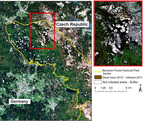
The study area covers the upper part of the Bavarian Forest National Park, the oldest national park in Germany, located at the eastern border of the federal state of Bavaria (49°3′19′′N, 13°12′49′′E) (Figure 1). This park, together with the adjacent Šumava National Park in the Czech Republic, forms one of the most extensive and contiguous forest landscapes in Central Europe. The elevation gradient spans over 800 m of montane and high montane areas (from 650 to 1453 m a.s.l.) with dominant southwest slopes (Bässler et al. 2009). The annual precipitation (mostly snowfall during winter) varies between 1200 and 1800 mm, and the average annual temperature ranges from 3.8°C (higher montane areas) to 5.8°C (hillsides) to 5.1°C (valleys) (Bässler, Müller, and Dziock 2010). The main forest communities include species occurring in the sub-alpine domain (Picea abies L. Karst and Sorbus aucuparia L.), on slopes (P. abies L., Abies alba Mill., Fagus sylvatica L., and Acer pseudoplatanus L.), and in valleys (P. abies L., S. aucuparia L., Betula pendula Roth, and Betula pubescens Ehrh.) (Cailleret, Heurich, and Bugmann 2014). The core zone of the national park is managed as a natural forest succession with a no-take policy (Müller et al. 2008). The forests were frequently affected by wind storms during the 1980s; wind-thrown Norway spruce trees provided habitat for the dispersal of the spruce bark beetle (I. typographus L.). In this study, we masked all other deciduous and mixed-forest types using the vector-based forest habitat type map provided by the national park administration to minimize the mixed tree species effect on spectral signatures and focused solely on spruce stands as the main hosts of spruce bark beetles.

Figure 1. Natural-color RapidEye scene of the study area in Germany. Brown indicates the dead trees (infested with bark beetles in 2011) extracted by the analysis of aerial photographs from 2012. White shading around brown areas indicates buffer zones of variable size around each infested area. The red box indicates a zoomed-in subset of the study area.

2.2. Remote sensing and reference disturbance data

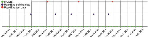
We used two series of remote sensing data, namely 8-day composites of MODIS reflectance acquired throughout the year 2011 and discrete acquisitions of multispectral RapidEye data for the available dates during the same year (Figure 2). The 8-day composites of MODIS (MOD09Q1) with a spatial resolution of 250 m were downloaded from the National Aeronautics and Space Administration (NASA) Land Processes Distributed Active Archive Center (https://lpdaac.usgs.gov/). The 8-day surface reflectance data consist of pixel values representing the best possible observation during the 8 days; these values are corrected for atmospheric gases and aerosols and are based on high observation coverage, low view angle, and absence of clouds or cloud shadow (Vermote, Roger, and Ray 2015). We used red and NIR bands to derive NDVI trajectories.

Figure 2. Overview of the data acquisition times in 2011. The green dots are the 8-day MODIS reflectance composites, purple dots are the RapidEye data used for training the data fusion, and red dots are the RapidEye data used as independent validation datasets.

RapidEye is a constellation of five similarly constructed satellites that enable frequent revisits over a given area. Each sensor consists of five spectral bands in blue, green, red, red edge, and NIR domains (Borg et al. 2013). We acquired level 3A RapidEye data, which includes radiometrically calibrated and orthorectified data at a spatial resolution of 5 m (Chander et al. 2013). Only scenes without cloud cover over the study area were selected for model training. We corrected the scenes atmospherically and topographically using ATCOR-3 (Richter and Schläpfer 2012) by applying a shuttle radar topography mission digital terrain model with a spatial resolution of 90 m.

Annual, vector-based reference datasets of disturbance history within the national park manually interpreted from film photographs (1988–2003) and digital orthophotos (2004 onwards) are available. The aerial images are products of flight campaigns carried out during the peak of vegetation activity during July each year. Infested forest patches comprising more than five trees at the red and gray stages of mortality were delineated by stereo photogrammetry. The resulting datasets cover all tree groups that show visible symptoms of disturbance each year and currently serve as the main management tools for bark beetle management (Heurich et al. 2010a; Latifi et al. 2014b). The reader is referred to Heurich et al. (2010a) for further descriptions of photogrammetric analysis of the orthophotos. We extracted polygons of infested trees in Norway spruce stands in 2012 from the dataset; the polygons ranged in size from ca. 30 m² to 24,661 m².

It has been reported that adult I. typographus individuals start swarming at the end of April and beginning of May each year (Lausch, Fahse, and Heurich 2011, Abdullah et al. 2017). However, there is an average 2–3 month time lag between the onset of the attack and changes in the spectral signature of the canopy that are visible in multispectral data (Kautz et al. 2014). Since these changes unlikely lead to red-stage tree mortality by the time the aerial surveys are conducted, we assumed that the delineated polygons of dead trees in 2012 are those in which infestations initiated in 2011. These polygons were then taken as inputs in the subsequent buffer analysis.

2.3. Methods

2.3.1. Buffer analysis

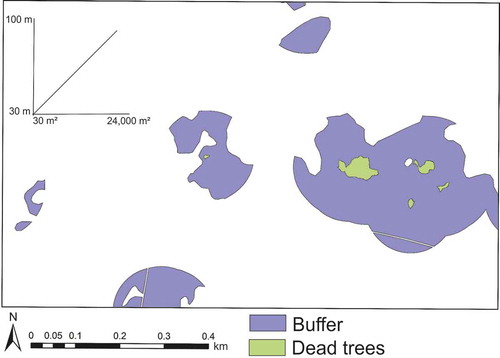
It has been reported that in bark-beetle-infested spruce stands the trees surrounding those felled by windthrows or those infested in an older attack are more vulnerable to subsequent infestations (Fahse and Heurich 2011; Kautz et al. 2011). The distance to the nearest infested patches is one of the crucial factors affecting bark beetle dispersal in the Bavarian Forest National Park and the neighboring Šumava National Park (Lausch, Fahse, and Heurich 2011; Hais et al. 2016). Owing to the absence of observation data of early phases of tree mortality within the Bavarian Forest National Park, we inserted buffers around the dead tree patches as a proxy zone, where a subsequent infestation is most likely be happen. With regard to the working spatial resolution of our study (5 m), we considered the infested patches extracted from aerial imagery (as described in Section 2.2) as the core units of forest disturbance and inserted buffer zones of the same shape around each patch as the zone in which the likelihood of beetle dispersal and new infestations is highest. Owing to the substantially variable sizes of the infested patches (ranging from 30 to >24,000 m²), we implemented variable buffer sizes; we simply used radii that increased in a linear ratio proportional to the size of the infested spruce patches. This resulted in radii surrounding the infested patches ranging from 30 m (for a 30 m² infested patch) to 100 m (for a 24,661 m² infested patch), which is roughly analogous to the concept of source and sink cells in infestation dynamics (Chen and Walton 2011). Similar to the stand selection noted above, the buffer zones were also constrained by the surrounding Norway spruce stands (Figure 3). By doing this, we assumed these buffer zones are the spatial domains of potential invasion of any upcoming beetle disturbance, and thereby excluded the newly opened windthrow areas from which additional attacks could be started. The relationship can be quantified as , with being the buffer radius and being the size of infested spruce patches.

Figure 3. An example of variable buffers (purple) inserted around polygons of dead trees (green) of 2012. The linear relationship between the polygon and buffer sizes is shown in the upper-left corner.

2.3.2. Spatiotemporal data fusion

In recent years, the remote sensing community has increasingly become interested in fusing spatiotemporal characteristics of different image datasets to generate synthetic data with fine resolutions (Camps-Valls et al. 2008; Huang and Song 2012; Chen and Xu 2014; Gao et al. 2015; Chen, Huang, and Xu 2016). In our context, the synthetic time series generated by such methods can be further used to imitate the phenology of forest stands throughout the growing season by means of original reflectance or the derived vegetation indices, from which diverse phenology metrics can be derived (Jönsson and Eklundh 2002; Buma, Pugh, and Wessman 2013).

Several data fusion algorithms exist, including the construction-based methods STARFM and ESTARFM, in which the synthetic imagery is generated by a weighted sum of the neighboring spectrally similar pixels from higher spatial resolution data with lower temporal resolution and lower spatial resolution data with higher temporal resolution (Gao et al. 2015). Another category includes the unmixing-based models (Chen, Huang, and Xu 2016), in which the focus is on preserving the spectral richness and conformity with unmixing techniques that downscale the lower spatial resolution data to higher resolution synthetic data. The FSDAF (Zhu et al. 2016) is a state-of-the-art example of such methods, in which a spectral unmixing and a thin plate spline (TPS) interpolation are combined. The method enables a simultaneous prediction of changes in gradual phenology and type, with motivations for further tests and validations in varying domains (Chen, Huang, and Xu 2016). The method might be useful for further tests across heterogeneous image scenes (Knauer et al. 2016), and the method has been mathematically described by Zhu et al. (2016). Briefly, it works as follows (Figure 4).

Figure 4. The workflow of FSDAF image fusion. The abbreviations t1 and t2 have been explained in Section 2.3.2.

The algorithm consists of six steps: (1) classification of the fine-resolution image at the initial time step (t1); (2) estimation of the temporal change of each class in the coarse-resolution image from the initial to the prediction time steps (t2); (3) prediction of the fine-resolution image at t2 using the class-level temporal change, followed by calculation of residuals at each coarse pixel; (4) prediction of the fine-resolution image from the coarse image at t2 with a TPS interpolation; (5) distribution of residuals based on TPS prediction; and (6) final prediction of the fine-resolution image using information from the neighborhood.

We applied the synthetic 8-day RapidEye-like composites of MODIS band 1 and band 2 to derive the NDVI curve (8-day temporal resolution) throughout the year 2011, which resulted in a total of 46 input variables for the subsequent classification. The NDVI values were extracted at the locations of each infested spruce patch in 2011 and from the surrounding infestation-likelihood buffer to form binary classes for classification.

For the dates for which both RapidEye and MODIS reflectance data were available (blue and red dots in Figure 2), we divided the number of RapidEye data points into five training and three independent hold-out test datasets, and correlated the real and the synthetic reflectance to the hold-out validation datasets.

2.3.3. Classification of synthetic data

We applied a random forest approach based on conditional inference trees (cforest) to explore all possible 8-day NDVI time points for separating the infested and the surrounding buffer classes. cforest copes with correlated input variables (the common case in remote sensing-assisted models), which might bias the classical random forest variable importance (Strobl et al. 2007). This is crucial, particularly when applying random forest in causal analyses, where the main aim is to select variables (here image dates) that best separate binary classes. In such analyses, the input spectral parameters are usually highly correlated (Dahms et al. 2016).

The classification was conducted with all 46 synthetic NDVI time steps as input variables and an iterative process of 100 repetitions. The results were cross-validated by a fivefold cross-validation, in which accuracy diagnostics, i.e., overall accuracy, P-values of overall accuracy, and McNemar’s test, were calculated. The selected results were extrapolated using random forest over the entire study area to provide wall-to-wall maps of infested and possibly infested areas. Random forest was chosen for the final mapping because of its slightly higher predictive performance compared to conditional inference trees. Furthermore, class-specific conditional probability surfaces of the positive class allocation were also mapped by taking the fraction of votes received for each class (Breiman 2002; Latifi et al. 2014b). The entire processing chain (image fusion, NDVI, sampling, classification, and validation) was implemented in an open-source domain in R (R Development Core Team 2017) using the R packages party (for conditional inference trees), randomForest (for random forest classification), and caret (for cross-validation).

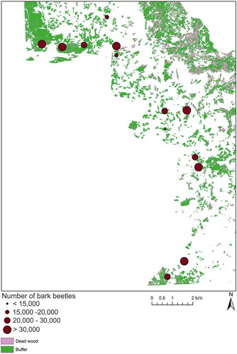
As an additional quantitative validation, we compared a portion of the classification results against the overlapping bark beetle trapping data along 13 sampling stations in which the sampled beetles were counted for a time period between 1 April and 30 September 2011. The data originally stemmed from a 5-year monitoring inside the management zone of the national park and the surrounding commercial forests (Lobinger 2016). Theyson-type pheromone traps with PHEROPRAX® (BASF) lures were mounted in forest gaps more than 30 m away from the next forest edge to avoid trap-induced green attacks (Schlyter 1992). The distance between single traps was about 1000 m, which took a critical radius of infestation of 500 m from infestation spots (Angst, Rüegg, and Forster 2012; Stadelmann et al. 2014).

We aggregated trap data from 13 stations overlapping with a portion of our study site and compared the beetle counts in traps against the area classified as dead trees (i.e., potentially infested in 2011) within a buffer of 100 m around the trapping stations (Figure 5). The 100 m buffer was selected based on existing reports on the zone of influence of bark beetles around their emerging spatial domains of infestation (Wichmann and Ravn 2001; Stadelmann et al. 2014). Unfortunately, common remote sensing time series from RapidEye data do not provide the desired temporal resolution. By contrast, synthetically generated time series provide much more frequent data for missing time points and thus allow a more precise determination of the influence of bark beetle infestation on forest stands.

Figure 5. Location of the pheromone traps overlapping a portion of the study site and the density of sampled beetles overlaid on a classification of synthetic RapidEye NDVI.

3. Results

3.1. Validation of synthetic reflectance from FSDAF method

We determined the correlations between the synthetic data and the hold-out independent validation RapidEye data for three selected dates throughout the growing season (Figure 6). On 19 April (leaf unfolding), 12 July (peak of growth period), and 22 October 2011 (autumn coloring), r² = 0.54, 0.53, and 0.53, respectively; root mean square error = 0.13, 0.13, and 0.13, respectively; and mean absolute error = 11.53, 11.44, and 11.59, respectively. Overall, only a marginally higher r² was observed at the leaf unfolding/beginning of flowering phase compared to the peak of growth period/mature leaf and the autumn coloring phases.

Figure 6. Scatterplots showing the correlation between the original independent validation and synthetic RapidEye data using the FSDAF method for 19 April (a), 12 July (b), and 22 November 2011. The 1:1 lines are dashed; the regression lines are solid. See text for values.

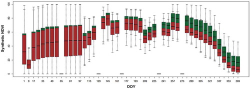
We compared NDVI curves derived from synthetic RapidEye data with 8-day temporal resolution in 2011 across infested spruce patches and the variable buffer zones of 2012 (Figure 7). The comparison clearly showed an increasing difference between the spectral responses of the two classes that starts approximately on the composite generated on day 209 of the year (28 July) and continues almost constantly until the end of the year.

Figure 7. The NDVI range from 8-day composites of synthetic RapidEye data for 2011 overlaid on the locations of dead tree polygons (red) and buffered polygons (green) in 2012. On the missing dates, no cloud-free MODIS data were available. DOY refers to “day of year.”

3.2. Selection of crucial dates and classification

The results of cforest classification applied on the input synthetic NDVI datasets results complemented the visual observations shown in Figure 7. The mean decrease error for 100 repetitions of cforest classification revealed multiple days throughout the year on which the dead wood and buffer (not infested) classes can be separated, with some important dates distributed throughout the year (e.g., days 137, 145, 161, and 249 of the year). However, the most important date for separating the classes was on day 281 of the year (8 October). This specific peak cannot be observed by only comparing the two NDVI curves (Figure 8), but it is unveiled by the cforest variable importance (Figure 8) and can be further considered for early detection of bark beetle mortality in the preceding year.

Figure 8. Results of conditional variable importance as mean decrease in accuracy of input image dates based on 100 repetitions of cforest.

When we tested the different numbers of variables randomly sampled at each split (mtry) values, the stability of the random forest classification was revealed. By selecting a range of values including mtry = 2 (smallest number of predictors), mtry = 46 (maximum number of predictors), and mtry = 24 (half of the number of predictors), both extreme and average numbers of randomly sampled variables at each split were covered. The classification results obtained by all three values did not significantly differ.

The overall accuracy of cforest ranged between 0.61 for mtry (input candidate variables at each node) = 2 and 0.67 for mtry = 24 or 46. Since random forest classification was associated with slightly higher predictive accuracy than cforest (Table 1), we used random forest for wall-to-wall mapping.

Table 1. Accuracy assessment of the random forest classification of binary classes.

		Reference data
		Dead trees	Buffered zone	Sum classified
Data	Dead trees	303	197	500
	Buffered zone	103	397	500
	Sum reference	406	594

The classes include dead trees and variable buffered zones from 2012, and the independent variables include NDVI image dates from 46 synthetic RapidEye data made throughout 2011.

Overall accuracy = 0.70, overall accuracy P-value = 8.832839e-38, McNemar’s test P-value = 7.901764e-08.

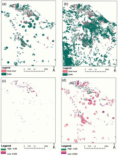
The wall-to-wall random forest map of mean classification results, map of early-infested patches, and class-specific classification probabilities for both disturbance classes showed varying degrees of probabilities for separating the tree mortalities in advanced and early stages (Figure 9). The general tendency was toward more confident classification of larger and more spectrally homogenous patches.

Figure 9. Examples of random forest maps of predicted classes and their classification probabilities. (a) Polygon-based classification, (b) wall-to-wall classification, (c) polygon-based classification probability of dead tree class, and (d) polygon-based classification probability of buffered zones. For clarity, all maps show only a subset of the entire study site.

When we compared the classification with bark beetle trapping data, we observed a significant positive correlation between the aggregated number of captured beetles per trap per year and the area classified as dead trees within its surrounding buffer (Pearson correlation = 0.57, P-value = 0.041, P ≤ 0.05) (Table 2). Most stations in which >30,000 beetles were counted showed a large share of trees classified as dead in their surroundings.

Table 2. Aggregated numbers of beetles counted per trap between 1 April and 30 September 2011 compared with the area classified as dead trees from synthetic RapidEye data in a buffer zone of 100 m radius around each trap.

Trap ID	Area classified as dead trees (m^2)	Beetle count in traps
1	8175	34,988
2	3150	31,488
3	6300	27,736
4	13,275	32,975
5	2625	19,408
6	950	24,249
7	575	13,464
8	150	24,909
9	4100	38,801
10	12,250	35,227
11	6725	22,908
12	1750	18,512
13	6050	42,630

4. Discussion

We derived a synthetic remote sensing time series by blending MODIS and RapidEye data and assessed its applicability for tree mortality mapping within a workflow based on remote sensing. One main objective was to identify the time steps in a remote sensing time series that are most important for classifying bark beetle infestation before the consequent dead trees are captured during the next year’s aerial survey. The most important time step as shown by cforest variable importance was at the beginning of October. This date might not be early enough to plan an effective infestation management for the upcoming year, compared to an ideal, but infeasible, early detection in July. Nevertheless, the date helps to map the areas most likely infested and in earlier stages of tree mortality, and it is earlier than when areas can be identified by aerial surveys in the following July or August.

Concerning the first research question, the results of our synthetic RapidEye data validated against independent validation data showed comparatively lower accuracies than a number of recent studies that blended MODIS with higher resolution data, such as RapidEye (Tewes et al. 2015) and SPOT 5 (Zheng et al. 2016). The performance of our validation stems most likely from differences in the spectral behavior of land-cover types in the study sites. We tested data fusion over heterogeneously structured spruce stands of the national park and achieved correlations of up to 0.54; other studies achieved an average r² of 0.85 and 0.79 over semi-arid rangelands (Tewes et al. 2015) and agricultural croplands (Zheng et al. 2016), respectively, both of which used reconstruction-based fusion methods that require a large amount of input data. By contrast, the FSDAF method has been distinguished for its flexibility in terms of limited input data and for being able to predict both gradual and land-cover type changes (Zhu et al. 2016). The latter work is a comparative study in which FSDAF exceeded both STARFM and unmixing-based data fusion for blending Landsat with MODIS data over a terrain consisting of croplands and natural vegetation, but no heterogeneous forest. Thus, we think that the results achieved in our implementation are realistic with regard to the challenging and mixed terrain with which we dealt. Comparative studies of different fusion methods were beyond the scope of our study, but might be beneficial in the future. In the context of FSDAF, we used an unsupervised ISODATA classification to estimate the temporal change of each class. Future work could use a supervised classification to obtain the temporal changes in each thematic class (e.g., different tree species or land-cover types).

The straightforward vegetation metric NDVI largely serves as a proxy that reflects the status of vegetation photosynthetic activity and amount of chlorophyll (Gamon et al. 1995; Gamon et al. 2015); it is thus assumed that the NDVI is affected by tree mortality. Coops et al. (2006) observed a significant difference between QuickBird’s high-resolution NDVI values of non-infested trees to those of advanced (i.e., red and gray) stages of tree mortality induced by the mountain pine beetle, but in a monotemporal context. Concerning the second research question, our approach revealed that at a spatial resolution of 5 m of synthetic RapidEye data in a given year, it might be possible to track the spectral behavior of infested stands by looking at the locations of dead trees and their surroundings in the following year. As shown here, increasing discrepancies between the spectral signals within pure spruce stands can be observed in the period following the peak vegetation activity until the end of the year. Such trends cannot be easily revealed in the presence of temporally discrete but spatially higher-resolution data; the trends depend on the frequency and chronological distribution of the available cloud-free data. By contrast, temporally continuous MODIS data enable such trends to be tracked. MODIS-based time series are successful in detecting large-scale disturbance locations but not in estimating the disturbance intensity when classification is the main goal (Eklundh, Johansson, and Solberg 2009). They also suffer from their insufficient spatial resolution for landscape-level analysis.

Following the highest level of epidemic bark beetle infestations in the mid-1990s in the national park, both the total extension of infested areas and size of individual patches have decreased since 2007 (Lausch, Heurich, and Fahse 2013), which resulted in a very patchy distribution of smaller infested areas. The infested patches of Norway spruce stands started at the size of a single Landsat pixel (30 × 30 m) and mostly included small segments that cannot be captured by Landsat-like data (see an overview in Figure 1). Therefore, we focused on producing RapidEye-like data with higher spatial resolution. We tried to incorporate the Norway spruce phenology and the peak level of insect damage in the timing of data acquisition (i.e., five RapidEye scenes for training and three scenes for testing), as according to Gärtner, Förster, and Kleinschmit (2016) and Meigs, Kennedy, and Cohen (2011).

However, it should not be considered as a typical means of obtaining high-resolution base images for fusion purposes since factors such as cloud cover, haze, and snow could seriously constrain their availability. We were constrained by RapidEye image availability throughout consecutive years, which obliged us to focus on one year, namely 2011, in which the highest number of appropriate data could be found. This is not a major issue for a study at the experimental level, but it can be prohibitive for practical and long-term applications. Blending RapidEye data with other high-resolution Earth observation products, such as Copernicus Sentinel-2 data (spatial resolutions starting from 10 m) and Landsat 8 data (spatial resolution of 30 m) can supposedly provide better results. This is, however, constrained by, e.g., extensive cloud cover over mountainous forest areas and the size of infested patches. Alternatives could be the combining of higher-resolution imagery from multiple sensors, such as RapidEye (constellation, 5.5 days revisit time) + Sentinel-2 (5 days revisit time), to reach the desired frequency and distribution of datasets used for training throughout the years. This would extend the current methodology by using longer time series, which would provide results beyond a single, inter-annual context.

Although information derived from remote sensing expands the scale of phenological observations beyond those that are possible via traditional field-based methods (Tang et al. 2016), validating satellite-based products with field-based phenology is generally challenged by the limited number or lack of observations for specific forest types, e.g., infested spruce stands in the International Phenological Gardens. Because of this general shortage and/or infeasibilities of field-based phenological observations with high temporal resolution over forested areas (Denny et al. 2014), we focused on implementing a workflow that largely relied on remote sensing data by using continuous MODIS and discrete RapidEye acquisitions.

The NDVI curves of our fused data well reflect the common phenological behavior of spruce stands throughout the year. For example, they are consistent with the common bud break of Norway spruce stands in the test site, which normally occurs on approximately day 120 of the year and thus leads to an increase in the amount of NDVI. When we overlaid the locations of dead tree and buffer regions from 2012 on the 2011 image time series, the difference between the NDVI values of the two classes became larger as the growing season advanced after the bud break, and led to the most important separation point on day 281 of the year, as shown by cforest variable importance. Although no similar study of insect disturbances was available for comparison with our study, that of, e.g., Van Leeuven et al. (2010), which used dense MODIS time series at lower spatial resolution, pointed out similar differences in metrics, such as peak and end-of-season activities between undisturbed stands and stands disturbed by wildfire.

The results of variable selection presented here can be potentially useful for assessing the best point of time at which the visual symptoms of infestation appear on the tree crowns. When this framework is used to extrapolate results to the entire area (Figure 9(a,b)), the results can be used as a proxy to delineate the expected infested areas of the following year. In addition, comparison of classification results with beetle-trap data suggested a reasonable agreement between sampled beetle count and tree mortality in the following year. This supports the use of our workflow for guiding future fieldwork monitoring within potentially vulnerable spruce stands. Despite this promising observation, mark-release-recapture experiments using pheromone traps are only partially able to reflect the true distribution of individual beetles (Kautz et al. 2016). In our particular context, (1) the observed association does not mean an unconditional dependence of infestation on the sampled number of caught beetles, and (2) beetles dispersed from the surrounding (but masked out) mixed stands might also contribute to the sampled number at each trap located in a spruce stand.

Last but not least, although this solely NDVI-based approach yielded satisfactory mapping accuracies, our visual comparisons of the classified infestations with those delineated as dead trees on 2012 aerial photographs showed that the RapidEye-based approach results in a considerable number of false-positive classifications. That is, some areas that are not seen on the aerial photos of the following year are falsely classified as infested, although most of the areas classified as infested in 2011 synthetic data exactly matched those delineated as dead trees in 2012 aerial photographs. We acknowledge that an approach solely based on NDVI is not enough to fully reflect infestation dynamics, as many other climatic and topographic drivers and some unknown factors are involved in spatiotemporal patterns of I. typographus in the national park (see Lausch, Heurich, and Fahse 2013 for an in-depth analysis). However, such remote sensing products can aid forest managers in guiding more in-depth disturbance field observations in subsequent years to identify specific time spans and locations (Frantz et al. 2017), which would result in saving costs and logistics.

5. Conclusions

This study was mainly motivated by the mostly site-specific earlier results of classical supervised classification of passive optical data for the detection of tree mortality, which were challenged mainly because of inconsistencies between field- and image-based disturbance classes and the time lag between satellite and aerial reference data (see Section 1). We applied an FSDAF data fusion approach to blend MODIS and RapidEye reflectance and created 8-day composites of synthetic RapidEye-like NDVI data for analyzing Norway spruce mortality induced by bark beetles. The fusion results moderately correlated with independent validation data from real RapidEye datasets, mainly because of the complexities of land-surface and heterogeneous forest structures across the Bavarian Forest National Park. We assumed that the dead trees delineated on 2012 aerial photographs were those in which infestations initiated in 2011. Variable buffers around the dead trees in 2012 combined with conditional inference variable selection showed that spectral information after the peak of the growth season in preceding year (2011) can be used to discriminate between infested trees and their surroundings. Also the significant correlations of classification data with field-based beetle count data confirmed the results. This experimented approach enables delineation of the infested areas before they are delineated as dead trees on aerial photos around 1 year later. The results offer potential implications for rapid and cost-effective monitoring of bark beetle outbreaks using satellite data, which is of great interest for both landscape-level administrative and research tasks.

Highlights

• Forest disturbance data combined with synthetic optical data identified stands vulnerable to bark beetle infestation.

• We fused RapidEye and MODIS data to create synthetic intra-annual NDVI data at a spatial resolution of 5 cm.

• Day 281 of the year was the most critical date for recognizing infestation in the previous year.

• Dates selected based on trajectories of NDVI data were significantly correlated with field-based beetle count data.

Acknowledgements

MODIS products were provided by the USGS and NASA. Daniel Baron and Philipp Glaser contributed to an earlier preliminary study dealing with the phenology of infested stands that was funded by a research grant of the Faculty of Philosophy, University of Würzburg. We acknowledge the support of the Data Pool Initiative for the Bohemian Forest Ecosystem. The Bavarian Forest National Park financed a professional English proofreading of the revised manuscript.

Disclosure statement

No potential conflict of interest was reported by the authors.

Additional information

Funding

The study was facilitated by the provision of RapidEye data by the German Aerospace Center (Deutsches Zentrum für Luft- und Raumfahrt e.V.) as part of the RapidEye Science Archive (Proposal ID 00207).

References

- Aakala, T., T. Kuuluvainen, T. Wallenius, and H. Kauhanen. 2011. “Tree Mortality Episodes in the Intact Picea Abies-Dominated Taiga in the Arkhangelsk Region of Northern European Russia.” Journal of Vegetation Science 22 (2): 322–333. doi:10.1111/jvs.2011.22.issue-2.
- Abdullah, H., R. Darvishzadeh, A.K. Skidmore, T.A. Groen, and M. Heurich. 2017. “European Spruce Bark Beetle (Ips Typographus, L.) Green Attack Affects Foliar Reflectance and Biochemical Properties.”international.” International Journal Of Applied Earth Observation and Geoinformation" 64: 199-209. doi: 10.1016/j.jag.2017.09.009.
- Angst, A., R. Rüegg, and B. Forster. 2012. “Declining Bark Beetle Densities (Ips Typographus, Coleoptera: Scolytinae) from Infested Norway Spruce Stands and Possible Implications for Management.” Psyche: A Journal of Entomology 2012: 321084.
- Bässler, C., B. Förster, B. C. Moning, and J. Müller. 2009. “The Bioklim Project: Biodiversity Research between Climate Change and Wilding in a Temperate Montane Forest: The Conceptual Framework.” Forest Ecology, Landscape Research and Nature Conservation 7: 21–34.
- Bässler, C., J. Müller, and F. Dziock. 2010. “Detection of Climate-Sensitive Zones and Identification of Climate Change Indicators: A Case Study from the Bavarian Forest National Park.” Folia Geobotanica 45 (2): 163–182. doi:10.1007/s12224-010-9059-4.
- Borg, E., H. Daedelow, K.-D. Missling, and M. Apel. 2013. “RapidEye Science Archive: Remote Sensing Data for the German Scientific Community.” In: 5th RESA Workshop “Data for Science: From the Basics to the Service”: 5–20, Neustrelitz, 20.–21.3.2012, Eds. E. Borg, H. Daedelow, and R. Johnson, GITO mbH Verlag, Berlin. ISBN 978-3-95545-002-1.
- Breiman, L. 2002. “Manual on Setting Up, Using and Understanding Random Forests V3.1.” http://oz.berkeley.edu/users/breiman/Using_random_forests_V3.1.pdf.
- Buma, B., E. T. Pugh, and C. A. Wessman. 2013. “Effect of the Current Major Insect Outbreaks on Decadal Phenological and LAI Trends in Southern Rocky Mountain Forests.” International Journal of Remote Sensing 34 (20): 7249–7274. doi:10.1080/01431161.2013.817717.
- Cailleret, M., M. Heurich, and H. Bugmann. 2014. “Reduction in Browsing Intensity May Not Compensate Climate Change Effects on Tree Species Composition in the Bavarian Forest National Park.” Forest Ecology and Management 328: 179–192. doi:10.1016/j.foreco.2014.05.030.
- Camps-Valls, G., L. Gomez-Chova, J. Munoz-Mari, J. L. Rojo-Alvarez, and M. Martinez-Ramon. 2008. “Kernel-Based Framework for Multitemporal and Multisource Remote Sensing Data Classification and Change Detection.” IEEE Transactions on Geoscience and Remote Sensing 46 (6): 1822–1835. doi:10.1109/TGRS.2008.916201.
- Chander, G., M. O. Haque, A. Sampath, A. Brunn, G. Trosset, D. Hoffmann, and C. Anderson. 2013. “Radiometric and Geometric Assessment of Data from the RapidEye Constellation of Satellites.” International Journal of Remote Sensing 34 (16): 5905–5925. doi:10.1080/01431161.2013.798877.
- Chen, B., B. Huang, and B. Xu. 2016. “A Hierarchical Spatiotemporal Adaptive Fusion Model Using One Image Pair.” International Journal of Digital Earth. doi:10.1080/17538947.2016.1235621.
- Chen, B., and B. Xu. 2014. “A Unified Spatial-Spectral-Temporal Fusion Model Using Landsat and MODIS Imagery.” In: The 3rd International Workshop on Earth Observation and Remote Sensing Applications (EORSA), 2014. 11-14 June 2014, Changsha, China.
- Chen, H., and A. Walton. 2011. “Mountain Pine Beetle Dispersal: Spatiotemporal Patterns and Role in the Spread and Expansion of the Present Outbreak.” Ecosphere 2: 1–17. doi:10.1890/ES10-00172.1.
- Chytry, M., and L. Tichý. 1998. “Phenological Mapping in a Topographically Complex Landscape by Combining Field Survey with an Irradiation Model.” Applied Vegetation Science 1: 225–232. doi:10.2307/1478952.
- Coggins, S., N. Coops, and M. Wulder. 2010. “Estimates of Bark Beetle Infestation Expansion Factors with Adaptive Cluster Sampling.” International Journal of Pest Management 57 (1): 11–21. doi:10.1080/09670874.2010.505667.
- Coops, N. C., M. Johnson, M. A. Wulder, and J. C. White. 2006. “Assessment of QuickBird High Spatial Resolution Imagery to Detect Red Attack Damage Due to Mountain Pine Beetle Infestation.” Remote Sensing of Environment 103: 67–80. doi:10.1016/j.rse.2006.03.012.
- Dahms, T., S. Seissiger, E. Borg, H. Vajen, B. Fichtelmann, and C. Conrad. 2016. “Important Variables of a RapidEye Time Series for Modelling Biophysical Parameters of Winter Wheat.” Photogrammetrie, Fernerkundung, Geoinformation 2016 (5–6): 285–299. doi:10.1127/pfg/2016/0303.
- Denny, E. G., K. L. Gerst, A. J. Miller-Rushing, G. L. Tierney, T. M. Crimmins, C. F. E. Enquist, P. Guertin, et al. 2014. “Standardized Phenology Monitoring Methods to Track Plant and Animal Activity for Science and Resource Management Applications.” International Journal of Biometeorology 58: 591–601. doi:10.1007/s00484-014-0789-5.
- Eklundh, L., T. Johansson, and S. Solberg. 2009. “Mapping Insect Defoliation in Scots Pine with MODIS Time-Series Data.” Remote Sensing of Environment 133: 1566–1573. doi:10.1016/j.rse.2009.03.008.
- Fahse, L., and M. Heurich. 2011. “Simulating and Analysing Outbreaks and Management of Bark Beetle Infestations on a Stand Level.” Ecological Modelling 222: 1833–1846. doi:10.1016/j.ecolmodel.2011.03.014.
- Fassnacht, F., H. Latifi, A. Ghosh, P. Joshi, and B. Koch. 2014. “Assessing the Potential of Hyperspectral Imagery to Map Bark Beetle-Induced Tree Mortality.” Remote Sensing of Environment 140: 533–548. doi:10.1016/j.rse.2013.09.014.
- Fassnacht, F., H. Latifi, and B. Koch. 2012. “An Angular Vegetation Index for Imaging Spectroscopy Data – Preliminary Results on Forest Damage Detection in the Bavarian National Park, Germany.” International Journal of Applied Earth Observation and Geoinformation 19: 308–321. doi:10.1016/j.jag.2012.05.018.
- Frantz, D., A. Röder, M. Stellmes, and J. Hill. 2017. “Phenology-Adaptive Pixel-Based Compositing Using Optical Earth Observation Imagery.” Remote Sensing of Environment 190: 331–347. doi:10.1016/j.rse.2017.01.002.
- Gamon, J. A., C. B. Field, M. L. Goulden, K. L. Griffin, A. E. Hartley, G. Joel, J. Penuelas, and R. Valentini. 1995. “Relationships between NDVI, Canopy Structure, and Photosynthesis in Three Californian Vegetation Types.” Ecological Applications 5 (1): 28–41. doi:10.2307/1942049.
- Gamon, J. A., O. Kovalchuck, C. Y. S. Wong, A. Harris, and S. R. Garrity. 2015. “Monitoring Seasonal and Diurnal Changes in Photosynthetic Pigments with Automated PRI and NDVI Sensors.” Biogeosciences 12: 4149–4159. doi:10.5194/bg-12-4149-2015.
- Gao, F., J. Masek, M. Schwaller, and H. Hall. 2006. “On the Blending of the Landsat and MODIS Surface Reflectance: Predicting Daily Landsat Surface Reflectance.” IEEE Transactions on Geosciences and Remote Sensing 44: 2207−2218.
- Gao, F., T. Hilker, X. Zhu, M. Anderson, J. Masek, P. Wang, and P. Yang. 2015. “Fusing Landsat and MODIS Data for Vegetation Monitoring.” IEEE Geoscience and Remote Sensing Letters 3 (3): 47–60. doi:10.1109/MGRS.2015.2434351.
- Gärtner, P., M. Förster, and B. Kleinschmit. 2016. “The Benefit of Synthetically Generated RapidEye and Landsat 8 Data Fusion Time Series for Riparian Forest Disturbance Monitoring.” Remote Sensing of Environment 177: 237–247. doi:10.1016/j.rse.2016.01.028.
- Goodwin, N. R., S. Magnussen, N. C. Coops, and M. A. Wulder. 2010. “Curve Fitting of Time Series Landsat Imagery for Characterising a Mountain Pine Beetle Infestation Disturbance.” International Journal of Remote Sensing 31 (12): 3263–3271. doi:10.1080/01431160903186277.
- Hais, M., J. Wild, J. Berec, J. Brůna, R. Kennedy, J. Braaten, and Z. Brož. 2016. “Landsat Imagery Spectral Trajectories—Important Variables for Spatially Predicting the Risks of Bark Beetle Disturbance.” Remote Sensing (8): 687. doi:10.3390/rs8080687.
- Heurich, M., T. Ochs, T. Andersen, and T. Schneider. 2010a. “Object-Orientated Image Analysis for the Semi-Automatic Detection of Dead Trees following a Spruce Bark Beetle (Ips Typographus) Outbreak.” European Journal of Forest Research 129: 313–324. doi:10.1007/s10342-009-0331-1.
- Hilker, T., M. A. Wulder, N. C. Coops, J. Linke, G. McDermid, J. G. Masek, F. Gao, and J. C. White. 2009. “A New Data Fusion Model for High Spatial- and Temporal-Resolution Mapping of Forest Disturbance Based on Landsat and MODIS.” Remote Sensing of Environment 113: 1613–1627. doi:10.1016/j.rse.2009.03.007.
- Huang, B., and H. Song. 2012. “Spatiotemporal Reflectance Fusion via Sparse Representation.” IEEE Transactions on Geoscience and Remote Sensing 50 (10): 3707–3716. doi:10.1109/TGRS.2012.2186638.
- Jactel, H., and F. Vodde 2011. “Prevalence of Biotic and Abiotic Hazards in European Forests.” Tech. Rep. 86, EFI Technical Report 66, European Forest Institute. Accessed 21 Sep 2015. http://www.efi.int/files/attachments/publications/eforwood/efi_tr_66.pdf
- Jönsson, P., and L. Eklundh. 2002. “Seasonality Extraction by Function Fitting to Time-Series of Satellite Sensor Data.” IEEE Transactions on Geoscience and Remote Sensing 40 (8): 1824–1832. doi:10.1109/TGRS.2002.802519.
- Kautz, M. 2014. “On Correcting the Time-Lag Bias in Aerial-Surveyed Bark Beetle Infestation Data.” Forest Ecology and Management 326: 157–162. doi:10.1016/j.foreco.2014.04.010.
- Kautz, M., K. Dworschak, A. Gruppe, and R. Schopf. 2011. “Quantifying Spatio-Temporal Dispersion of Bark Beetle Infestations in Epidemic and Non-Epidemic Conditions.” Forest Ecology and Management 262 (4): 598–608. doi:10.1016/j.foreco.2011.04.023.
- Kautz, M., M. A. Imron, K. Dworschak, and R. Schopf. 2016. “Dispersal Variability and Associated Population-Level Consequences in Tree-Killing Bark Beetles.” Movement Ecology 4 (9): doi:10.1186/s40462-016-0074-9.
- Kautz, M., R. Schopf, and M.A. Imron. 2014. “Individual Traits as Drivers Of Spatial Dispersal and Infestation Patterns in a Host–bark Beetle System.” Ecological Modelling 273: 264–276. doi: 10.1016/j.ecolmodel.2013.11.022.
- Klein, W. 1982. “Estimating Bark Beetle-Killed Lodgepole Pine with High Altitude Panoramic Photography.” Photogrammetric Engineering and Remote Sensing 48: 733–737.
- Knauer, K., U. Gessner, R. Fensholt, and C. Kuenzer. 2016. “An ESTARFM Fusion Framework for the Generation of Large-Scale Time Series in Cloud-Prone and Heterogeneous Landscapes.” Remote Sensing 8: 425. doi:10.3390/rs8050425.
- Kulakowski, D., R. Seidl, J. Holeksa, T. Kuuluvainen, T. A. Nagel, M. Panayotov, M. Svoboda, et al. 2017. “A Walk on the Wild Side: Disturbance Dynamics and the Conservation and Management of European Mountain Forest Ecosystems.” Forest Ecology and Management 388: 120–131. doi:10.1016/j.foreco.2016.07.037.
- Latifi, H., B. Schumann, M. Kautz, and S. Dech. 2014a. “Spatial Characterization of Bark Beetle Infestations by a Multi-Date Synergy of SPOT and Landsat Imagery.” Environmental Monitoring and Assessment 186: 441–456. doi:10.1007/s10661-013-3389-7.
- Latifi, H., F. E. Fassnacht, B. Schumann, and S. Dech. 2014b. “Object-Based Extraction of Bark Beetle (Ips Typographus L.) Infestations Using Multi-Date Landsat and SPOT Satellite Imagery.” Progress in Physical Geography 38 (6): 755–785. doi:10.1177/0309133314550670.
- Lausch, A., L. Fahse, and M. Heurich. 2011. “Factors Affecting the Spatio-Temporal Dispersion of Ips Typographus (L.) In Bavarian Forest National Park: A Long-Term Quantitative Landscape-Level Analysis.” Forest Ecology and Management 261: 233–245. doi:10.1016/j.foreco.2010.10.012.
- Lausch, A., M. Heurich, and L. Fahse. 2013. “Spatio-Temporal Infestation Patterns of Ips Typographus (L.) In the Bavarian Forest National Park, Germany.” Ecological Indicators 31: 73–81. doi:10.1016/j.ecolind.2012.07.026.
- Lobinger, G. 2016. “Borkenkäfer-Monitoring Im Umfeld Des NP Bayerischer Wald.” AFZ-DerWald 12/2016: 48–52 (In German).
- Meigs, G. W., R. E. Kennedy, and W. B. Cohen. 2011. “A Landsat Time Series Approach to Characterize Bark Beetle and Defoliator Impacts on Tree Mortality and Surface Fuels in Conifer Forests.” Remote Sensing of Environment 115: 3707–3718. doi:10.1016/j.rse.2011.09.009.
- Menzel, A., and P. Fabian. 1999. “Growing Season Extended in Europe.” Nature 397: 659. doi:10.1038/17709.
- Müller, J., H. Bußler, M. Goßner, T. Rettelbach, and P. Duelli. 2008. “The European Spruce Bark Beetle Ips Typographus in a National Park: From Pest to Keystone Species.” Biodiversity and Conservation 17: 2979–3001. doi:10.1007/s10531-008-9409-1.
- Nielsen, M. M., M. Heurich, B. Malmberg, and A. Brun. 2014. “Automatic Mapping of Standing Dead Trees after an Insect Outbreak Using the Window Independent Context Segmentation Method.” Journal of Forestry 112 (6): 564–571.
- R Development Core Team. 2017. R: A Language and Environment for Statistical Computing. R Foundation for Statistical Computing. Vienna, Austria. Accessed 25 July 2015. http://www.R-project.org
- Raffa, K. F., B. H. Aukema, B. J. Bentz, A. L. Carroll, J. A. Hicke, M. G. Turner, and W. H. Romme. 2008. “Cross-Scale Drivers of Natural Disturbances Prone to Anthropogenic Amplification: The Dynamics of Bark Beetle Eruptions.” BioScience 58: 501–517. doi:10.1641/B580607.
- Richter, R., and D. Schläpfer. 2012. Atmospheric/Topographic Correction for Satellite Imagery: ATCOR- 2/3 Ver. 8.2 Beta User Guide. Accessed 25 July 2015. http://www.dlr.de/eoc/Portaldata/60/Resources/dokumente/5_tech_mod/atcor3_manual_2012.pdf.
- Schlyter, F. 1992. “Sampling Range, Attraction Range, and Effective Attraction Radius: Estimates of Trap Efficiency and Communication Distance in Coleopteran Pheromone and Host Attractant Systems.” Journal of Applied Entomology 114: 439–454. doi:10.1111/jen.1992.114.issue-1-5.
- Senf, C., R. Seidl, and P. Hostert. 2017. “Remote Sensing of Forest Insect Disturbances: Current State and Future Directions.” International Journal of Applied Earth Observation and Geoinformation 60: 49–60. doi:10.1016/j.jag.2017.04.004.
- Skakun, R., M. A. Wulder, and S. Franklin. 2003. “Sensitivity of the Thematic Mapper Enhanced Wetness Difference Index to Detect Mountain Pine Beetle Red Attack Damage.” Remote Sensing of Environment 86 (4): 433–443. doi:10.1016/S0034-4257(03)00112-3.
- Stadelmann, G., H. Bugmann, B. Wermelinger, and C. Bigler. 2014. “Spatial Interactions between Storm Damage and Subsequent Infestations by the European Spruce Bark Beetle.” Forest Ecology and Management 318: 167–174. doi:10.1016/j.foreco.2014.01.022.
- Strobl, C., A. L. Boulesteix, A. Zeileis, and T. Hothorn. 2007. “Bias in Random Forest Variable Importance Measures – Illustrations, Sources and a Solution.” BioMed Central Bioinformatics 8 (1): 307.
- Studer, S., R. Stöckli, C. Appenzeller, and P. L. Vidale. 2007. “A Comparative Study of Satellite and Ground-Based Phenology.” International Journal of Biometeorology 51: 405–414. doi:10.1007/s00484-006-0080-5.
- Tang, J., C. Körner, H. Muraoka, S. Piao, M. Shen, S. J. Thackeray, and X. Yang. 2016. “Emerging Opportunities and Challenges in Phenology: A Review.” Ecosphere 7 (8): e01436. doi:10.1002/ecs2.1436.
- Tewes, A., F. Thonfeld, M. Schmidt, R. J. Oomen, X. Zhu, O. Dubrovyk, G. Menz, and G. Schellberg. 2015. “Using RapidEye and MODIS Data Fusion to Monitor Vegetation Dynamics in Semi-Arid Rangelands in South Africa.” Remote Sensing 2015 (7): 6510–6534. doi:10.3390/rs70606510.
- Thom, D., and R. Seidl. 2016. “Natural Disturbance Impacts on Ecosystem Services and Biodiversity in Temperate and Boreal Forests.” Biological Reviews 91 (3): 760–781.
- Van Leeuwen, W. J. D., G. M. Casady, D. G. Neary, S. Bautista, J. A. Alloza, Y. Carmel, L. Wittenberg, D. Malkinson, and B. J. Orr. 2010. “Monitoring Post-Wildfire Vegetation Response with Remotely Sensed Time-Series Data in Spain, USA and Israel.” International Journal of Wildland Fire 19: 75. doi:10.1071/WF08078.
- Vermote, E. F., J. C. Roger, and J. P. Ray. 2015. MODIS Surface Reflectance User’s Guide (Collection 6). MODIS Land Surface Reflectance Science Computing Facility. http://modis-sr.ltdri.org
- Wichmann, L., and H. P. Ravn. 2001. “The Spread of Ips Typographus (L.) (Coleoptera, Colytidae) Attacks Follow-Ing Heavy Windthrow in Denmark, Analysed Using GIS.” Forest Ecology and Management 148: 31–39. doi:10.1016/S0378-1127(00)00477-1.
- Wulder, M., J. C. White, A. L. Carroll, and N. C. Coops. 2009. “Challenges for the Operational Detection of Mountain Pine Beetle Green Attack with Remote Sensing.” The Forestry Chronicle 85: 32–38. doi:10.5558/tfc85032-1.
- Zheng, Y., B. Wu, M. Zhang, and H. Zeng. 2016. “Crop Phenology Detection Using High Spatio-Temporal Resolution Data Fused from SPOT5 and MODIS Products.” Sensors 2016 (16): 2099. doi:10.3390/s16122099.
- Zhu, X., E. H. Helmer, F. Gao, D. Liu, J. Chen, and M. A. Lefsky. 2016. “A Flexible Spatiotemporal Method for Fusing Satellite Images with Different Resolutions.” Remote Sensing of Environment 172: 165–177. doi:10.1016/j.rse.2015.11.016.
- Zhu, X., J. Chen, F. Gao, X. Chen, and J. G. Masek. 2010. “An Enhanced Spatial and Temporal Adaptive Reflectance Fusion Model for Complex Heterogeneous Regions.” Remote Sensing of Environment 114: 2610–2623. doi:10.1016/j.rse.2010.05.032.