Supervised classification of electric power transmission line nominal voltage from high-resolution aerial imagery

Abstract

For many researchers, government agencies, and emergency responders, access to the geospatial data of US electric power infrastructure is invaluable for analysis, planning, and disaster recovery. Historically, however, access to high quality geospatial energy data has been limited to few agencies because of commercial licenses restrictions, and those resources which are widely accessible have been of poor quality, particularly with respect to reliability. Recent efforts to develop a highly reliable and publicly accessible alternative to the existing datasets were met with numerous challenges – not the least of which was filling the gaps in power transmission line voltage ratings. To address the line voltage rating problem, we developed and tested a basic methodology that fuses knowledge and techniques from power systems, geography, and machine learning domains. Specifically, we identified predictors of nominal voltage that could be extracted from aerial imagery and developed a tree-based classifier to classify nominal line voltage ratings. Overall, we found that line support height, support span, and conductor spacing are the best predictors of voltage ratings, and that the classifier built with these predictors had a reliable predictive accuracy (that is, within one voltage class for four out of the five classes sampled). We applied our approach to a study area in Minnesota.

Keywords:

• electricity
• transmission network
• machine learning
• GIS
• open data
• voltage ratings

1. Introduction

A significant shift has occurred with respect to the accessibility of geospatial energy data for the United States. Access to open data provides numerous benefits to researchers, government agencies, and emergency responders (Murray-Rust 2008; Donker, van Loenen, and Bregt 2016; Goodchild and Glennon 2010). Prior to 2017, however, public access to quality energy sector datasets was limited. While available in various forms from numerous data providers, ranging from government agencies to volunteered geographic information (VGI) platforms, the quality and accessibility of these data varied greatly. The US Energy Information Administration (EIA), for example, has a mandate to collect and publish a wide variety of energy data – particularly about electric power generation – for public use (Ambite et al. 2001). Public access to US electric power transmission data, however, has been more restrictive until recently. As of June 2017, the EIA hosted a selection of transmission line data provided by Ventyx, a private entity, on their website for public viewing. Due to license restrictions, however, these transmission line data did not include voltage information, and the viewing scale was limited. While still available from Ventyx directly, the cost associated with acquiring these data can be prohibitive for many users, and after having gained access, users are bound by the commercial license, which restricts data sharing.

As with the EIA, some electric utilities use the data acquired from commercial vendors to visualize and monitor their electric grid networks, such as Texas Entergy, Inc., a part of the Entergy Corporation, which, as of 6 June 2017 also cites Ventyx as the data source in the project maps listed on their website. Though some utilities publish project maps that include generalized representations of their infrastructure components with limited attribution on their website (examples include Tennessee Valley Authority, Xcel Energy Inc., and American Electric Power), the geospatial data displayed in these maps is rarely made available to users outside their respective organizations.

In contrast to the commercial and utility datasets, the OpenStreetMap (OSM) project allows unrestricted access to its database of transmission lines, but the quality of these data can be uncertain. The issue stems from the volunteered nature of the data, which are collected by volunteers with varying amounts of local knowledge and experience with data collection (Kerski and Clark 2012). As of 19 April 2017, to help the contributors determine line voltages, the OSM Wiki provides the following simple, yet problematic metric: “the length of the isolator (separating wires from tower) is 1 meter per 100,000 Volt.” Aside from the potential error involved in estimating these measurements from the ground, the metric stated above is not valid. The rating of an insulator depends on its design, material, and configuration, not its length directly (Shoemaker and Mack 2002, 13.13–13.24; CSEWEC 1964, 596). Therefore, in the absence of local knowledge or access to an alternate, authoritative source, the reliability of the voltage data in OSM is uncertain.

In 2017, the first government-owned alternative to the aforementioned datasets was made available to the public. In an effort to provide a shareable and reliable alternative to existing transmission datasets, the US Government sponsored Oak Ridge National Laboratory, Idaho National Laboratory, Los Alamos National Laboratory, and Argonne National Laboratory to develop foundation-level energy infrastructure data. As of 27 February 2018, this dataset remains available to the public via the Homeland Infrastructure Foundation-Level Data (HIFLD) Open platform (Oak Ridge National Laboratory Geographic Information Science and Technology Group et al. 2017). As of December 2017, the EIA’s US Energy Mapping System includes this dataset in lieu of the commercial dataset. Compared to alternatives, this government-off-the-shelf (GOTS) energy infrastructure dataset is more accessible and less costly than commercial products, and has more robust quality assurance and control measures when compared to VGI products (Oak Ridge National Laboratory Geographic Information Science and Technology Group et al. 2017). However, a review of this dataset found that 52% of transmission features were missing nominal voltage data (HIFLD Electric). The problem of missing data is not uncommon in open data and it presents a significant hindrance to data utility (Janssen, Charalabidis, and Zuiderwijk 2012). Geospatial transmission line data, particularly nominal voltage, are an important resource for data users. Transmission lines are designed to transmit energy over long distances through the “flow an electrical current against an electric potential,” or voltage (Kirtley 2010, 1). The nominal voltage of a transmission line is the voltage at which the line is designed to operate. A transmission dataset without nominal voltage data has limited utility for research and analysis because they are an essential input for power flow modeling and simulation (Simpson-Porco, Dörfler, Bullo 2016; Wang and Barnes 2014). Likewise, these data are valuable in the event of a natural disaster or power supply-related emergency, because they provide emergency planners and responders with a metric to gauge of the relative importance of transmission infrastructure assets.

This study draws from electric power systems, remote sensing, and machine learning disciplines to address the problem of missing nominal voltage data in open geospatial datasets. Supervised classification techniques have been applied to many problems in earth sciences and remote sensing literature (Li et al., 2013; Hong et al. 2015; Pham et al. 2016). However, the literature has yet to address the issue of missing nominal voltage data as a classification problem. In this study, we confront this problem by identifying and collecting predictors of nominal voltage, and developing and testing a methodology to estimate these data using a supervised classifier. Despite the limited availability of voltage data, inferences can be made about the nominal voltage of a transmission line based on its visual characteristics. Steel towers, for example, typically support very high voltage lines, while wood poles typically support lower voltage lines (Shoemaker and Mack 2002, 7.2, 8.1–8.10; Short 2004, 22). Likewise, right of ways are typically wider and support structures are usually taller when accommodating higher voltage transmission lines (Shoemaker and Mack 2002, 4.21; Rustebakke 1983, 131). We hypothesized that characteristics of transmission lines could be quantified as predictors of nominal voltage and collected using high-resolution aerial imagery. Once collected, these predictors were used to train a tree-based classifier, which was then tested using a validation set. Therefore, our contributions in this paper include: (i) identification of nominal voltage predictors and (ii) a novel application of supervised classification methods to estimate nominal voltage data.

The remainder of this paper is organized as follows. In Section 2, we present a detailed description of the data and the methods used. In Section 3, we present the results and discuss our findings. A short summary concludes the paper in Section 4.

2. Data and methods

2.1. Study area and source data

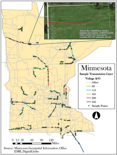
This study focused on a selection of transmission lines in the state of Minnesota (MN). There are five commonly used transmission voltages in Minnesota – namely, 69 kV, 115 kV, 161 kV, 230 kV, and 345 kV. The reason for selecting this study area was pragmatic, since it was the only area where authoritative transmission data could be acquired. Training data were created from data provided by the Minnesota Geospatial Information Office, which included a shapefile of three-thousand five-hundred twenty-eight transmission line features for the state of Minnesota (Minnesota Geospatial Information Office 2014). In this study, a selection of 56 transmission lines was used for training and testing purposes (see #1 and #2 in Figure 1). Predictors were collected via image interpretation and measurements from a combination of 1-meter and 0.3-meter resolution panchromatic imagery from ESRI’s World Imagery Service and DigitalGlobe (see #6 and #7 in Figures 1 and 3).

Figure 1. Workflow diagram of the methodology outlined in this study, including predictor collection, tree-based classification on sample points, validation set generalization, and final classification result.

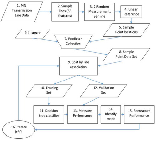
Figure 2. Map of electric power transmission lines in the state of Minnesota symbolized by nominal voltage, which were used to train and test the classifier in this study (adapted from Schmidt 2016, figure 8).

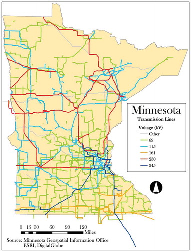
Figure 3. Map of electric power transmission lines used in this study symbolized by nominal voltage along with the location of their corresponding sample points. The inset shows a large-scale view of a sample line, sample points, and imagery that was used in this study (adapted from Schmidt 2016; figure 1).

2.2. Training data selection

The selection of training features was made based on voltage, spatial distribution, and positional accuracy. Of the total features in the Minnesota dataset, 3457 features belong to one of the five voltages used in this study: 69 kV, 115 kV, 161 kV, 230 kV, and 345 kV. A map of all transmission lines in this dataset – symbolized by voltage – is shown in Figure 2. Other voltages in the shapefile include 34 kV, 42 kV, 138 kV, 250 kV, 400 kV, and 500 kV, but these voltages were excluded from the study due to their rarity. At least eight features were selected as training lines for each voltage to adequately represent each voltage class. Table 1 shows the number of original line features in the Minnesota dataset by voltage class. Likewise, training features were selected from across the entire state to capture the effect of differing geographies on transmission line characteristics. For example, some transmission line owners may prefer using wood supports for 115 kV lines while others may favor steel supports for the same voltage. Furthermore, the training selection was limited to features with good positional accuracy, i.e., line features that were positioned near their corresponding transmission lines when examined against aerial imagery. Upon closer examination of the original dataset, numerous line features were excluded because their corresponding transmission lines could not be identified from aerial imagery.

Table 1. Count of Minnesota transmission line features, circuits, and sample lines by nominal voltage (reprinted from Schmidt 2016, table 1).

Voltage (kV)	Original line features	Original circuits	Sample lines
69	2218	503	13
115	785	287	14
161	152	30	10
230	176	42	11
345	126	24	8
Total	3457	886	56

From the sample of 56 transmission lines, a random sample of seven locations, hereafter referred to as sample points, were selected along each line feature (see #3 in Figure 1). For a given line, the location of these points was selected by generating seven random digits between zero and the total length of the line. The locations associated with these measurements are then georeferenced via linear referencing. These data were stored as point features in the file geodatabase. Predictor measurements, detailed below, were made in ArcMap software at each of these locations – 392 in total. A map of the sample lines and sample points used in this study is shown in Figure 3.

2.3. Predictor identification and collection

The predictors of nominal voltage identified and collected in this study were: support height, support span, conductor spacing, right of way width, insulator type, support type, construction material, number of circuits, and bundled conductors. These predictors were chosen based on information found in lineman guides and what could be feasibly identified from aerial imagery. All predictor measurements were collected and recorded manually within the ArcMap environment at each sample point location by overlaying the sample points on the aerial imagery and using the measuring tools or image interpretation techniques.

Support height was collected because higher voltage lines require greater clearances between the ground, or other obstacles, and the conductors, which necessitates taller supports (Shoemaker and Mack 2002, 36.28; Rustebakke 1983, 131). Support height was determined from 1-meter resolution aerial imagery from DigitalGlobe using mensuration tools available in ArcMap by measuring the support shadow from the center of the base of the support to the cross-section or post-insulator with the lowest conductor, rather than the top of the structure. These measurements required images with precise metadata on the date and time of collection since this information is necessary to determine the sun angle, which – when used in conjunction with the shadow length – can estimate the height of the structure.

The support span, conductor spacing, and right of way predictors were collected using the measuring tool in ArcMap. Support span was measured as the average distance between the support and the closest supports on the circuit. The conductor spacing, or phase spacing, predictor was measured as the average distance between each conductor of the circuit. Higher voltage lines require greater spacing between conductors to ensure insulation standards are met (CSEWEC 1964, 7–8, 34–37; Rustebakke 1983, 131–132). These measurements could not be collected for the sample points with vertically aligned conductors. The right of way width predictor was measured as the distance between the tree line on either side and perpendicular to the circuit. Typically, utilities maintain wider cuts through trees and vegetation to accommodate higher voltage lines and reduce the risk of circuit failure due to falling trees (Rustebakke 1983, 127; Shoemaker and Mack 2002, 4.21). An obvious constraint of this predictor is that it could not be collected in areas without trees or tall vegetation.

Insulator type, support type and material, bundled conductors, and multi-circuits were identified from electric power systems literature as possible predictors of nominal voltage. Post-insulators, as opposed to the string variation, are typically used on lower voltage transmission lines with lighter conductors (Shoemaker and Mack 2002, 13.13), making them a suspected predictor of voltage. Likewise, single pole supports are used in the construction of lower voltage transmission lines (Shoemaker and Mack 2002, 7.6), while H-frame and tower supports more commonly bear higher voltage lines due to their greater mechanical strength (7.9; 8.8). Wood-pole supports are generally most economical for lines up to 230 kV (Shoemaker and Mack 2002, 7.1–7.2) while the mechanical strength of concrete and especially metal makes them optimal for higher voltage lines (8.1–8.10). Some transmission line supports are designed to accommodate more than one transmission circuit, and based on observations of transmission lines in the MnGeo dataset, these multi-circuit supports appeared to be more prevalent among some voltage classes. Finally, bundled conductors are commonly used on high voltage transmission lines to reduce corona discharge, whereby the air surrounding an energized conductor is ionized, resulting in power loss (Shoemaker and Mack 2002, 4.22; Rustebakke 1983, 134–135).

These binary predictors were collected manually using image interpretation. Insulators were identified as being either string insulators, which are suspended beneath a cross-section or arm of the support, or post-insulators, which are attached above a cross-section or mounted perpendicularly to a single pole support. Generally, insulator type was determined by first identifying the support type or by examining the support shadow. The support type were identified as ether a single pole or a double pole/tower. The support material was categorized as wood or metal/concrete. The predictor for bundled conductors indicated whether each phase of the current was carried by more than one conductor. Ideally, this variable would be measured on a continuous scale, since the number of bundled conductors tends to increase with higher voltage (Shoemaker and Mack 2002, 4.10), but making this distinction was infeasible using 0.3-meter imagery so a binary measurement was used. More detailed information about the proposed methodology is described by Schmidt (2016).

All predictors were evaluated according to their mean variable importance rank – a normalized goodness measure of all partitions where the predictor was used as a primary or surrogate variable (Therneau and Atkinson 2017). For each tree, variable importance was sorted and ranked between 1 and 9, with lower ranks corresponding to greater variable importance in that model.

2.4. Classification

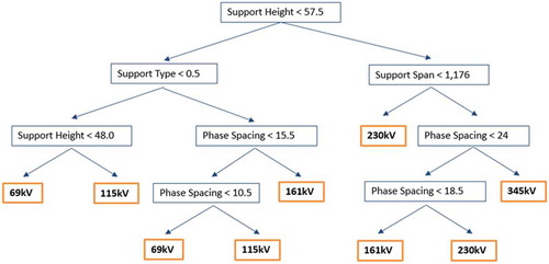
This study employed classification trees due to their simplicity and suitability for qualitative variables. Although decision tree-based methods do not perform as well as other classifiers (Amancio et al. 2014; Singh et al. 2012), they can be interpreted easily due to their transparent segmenting process (Quinlan 1986). Likewise, classification trees are well-suited for both continuous and discrete variables (James et al. 2013; Quinlan 1986), of which there were many in this study. For the purposes of this foundational study, weaker performance was an acceptable trade-off for greater transparency. This study was primarily concerned with a new application of classification methods, and therefore, the framework of the overall voltage classification method must be affirmed before additional, more complex classifiers are introduced. An example of a classification tree produced in this study can be seen in Figure 4.

Figure 4. An example of a classification tree produced during this study using the rpart package in R software (reprinted from Schmidt 2016, figure 2).

Classification trees in this study were created with the R software using the rpart package. The rpart module uses a recursive partitioning method that repeatedly partitions observations using maximal impurity reduction criteria, or rules that attempt to split the data such that the impurity, or heterogeneity, of nodes are minimized. To avoid overfitting a model to the training data, rpart prunes the tree by calculating a complexity parameter (cp), or cost associated with adding additional partitions to the tree. A lower cp results in more splits and increased risk of overfitting the training data, so rpart also performs 10-fold cross-validation for each additional split (Therneau and Atkinson 2017). Selecting the complexity parameter tied to the lowest cross-validation error is an attempt to parse the tree to a size that adequately classifies the observations without overfitting the training set.

To train and test the tree, the sample point dataset was divided into a training dataset and a validation dataset. At the sample line level, the data were divided into two equal halves with 196 sample points from 28 sample lines in each half. The first half was used to train the classification tree (see #10 in Figure 1), while the other half was set aside to test the performance of the tree (see #12 in Figure 1). Since the performance of the classification depends greatly on which samples were used in training and which were set aside for testing, this splitting process was performed randomly in 30 iterations (see #16 in Figure 1). In this way, sample points from the same sample line were not used to both train and test the classification; rather, all sample points belonging to each individual sample line were either used for training or testing purposes.

To measure the performance of the classifier (see #13 in Figure 1), the predictive accuracy and Kappa-coefficient were calculated and recorded for each validation set iteration. Likewise, the user accuracy and producer accuracy were calculated for each class in each iteration.

Finally, as a part of the post-processing, the output of the classifier was aggregated to the line features. Each line was assigned to the class with the highest frequency based on the mode of its sample points (see #14 in Figure 1). As an example, if four out of seven sample points associated with a single transmission line feature were predicted to be from the 161 kV class while the remaining three, the 230 kV class, the sample transmission line would be classified as the 161 kV class. In this way, outlier sample points that were misclassified can be smoothed over in the final cluster classification. The performance metrics were then re-measured to assess the impact of the mode identification on the classification (see #15 in Figure 1).

3. Results and discussion

3.1. Continuous predictor signatures

An examination of the predictors revealed a distinct signature, of varying strengths, with respect to voltage, especially among the continuous predictors. Support height, support span, and conductor spacing exhibit a distinct, positive relationship to voltage, as shown in Figure 5. The median of these predictors is higher with each consecutively higher voltage. The lowest median in each of these variables is found in the lowest voltage, 69 kV, while the highest median was associated with 345 kV, the highest voltage. To a degree, the right of way predictor shares this trend, but the signature was less distinct, which could be traced to numerous missing measurements as reported in Table 2.

Table 2. Summary statistics of continuous predictors by nominal voltage for sample points (adapted from Schmidt 2016, table 2).

	69 kV	115 kV	161 kV	230 kV	345 kV	Total
Sample points	91	98	70	77	56	392
Support height
Nulls	0	0	3	0	0	3
Support span
Nulls	0	0	0	0	0	0
Conductor spacing
Nulls	80	24	30	7	26	167
Right of way width
Nulls	65	60	67	47	48	287

Figure 5. Box plots of support height (upper left), support span (upper right), conductor spacing (lower left), and right of way width (lower right) symbolized by nominal voltage for sample points collected in this study.

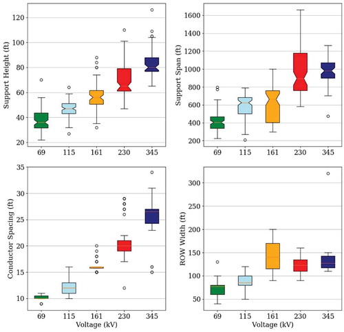
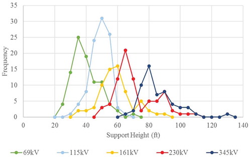
Furthermore, the variation of continuous predictor values differed notably across and within voltage classes. Compared to the 69 kV, 115 kV, and 345 kV classes, the 161 kV and 230 kV classes had much larger quartiles in the support span metric, suggesting that these latter classes have more variation than the former classes, as shown in Figure 5. With respect to support height, the differing shapes and widths of frequency curves in Figure 6 also illustrates intra-class variation. The 115 kV class has a narrow, near-normal curve while the 345 kV class features a wide, positively skewed shape. The 161 kV class, in contrast, is dispersed – lacking any strong clustering or dominance anywhere on graph; instead, the 115 kV and 230 kV signatures overshadow the 161 kV signature. After investigating, we found a geographic explanation for this problem.

Figure 6. Frequency plot of the support height predictor symbolized by nominal voltage for sample points collected in this study (adapted from Schmidt 2016, figure 3).

Figure 2 reveals a significant pattern in the distribution of transmission voltages within the state. The 161 kV class is only present in the southern part of the state, while the 230 kV class is only found in the middle and northern regions. Likewise, the 345 kV lines are predominantly located in the southern and middle regions, while the 115 kV class is most commonly found in the middle and northern regions. In short, there is little geographic overlap in the regions served by 161 kV and 345 kV lines and those served by 115 kV and 230 kV lines. The capacity of 161 kV lines makes them a middle ground between 115 kV and 230 kV lines, so the overlapping signatures of this class with the others should have been expected since the classification was performed at the state level. This suggests that careful consideration should be given to delineating the geographic region within which the classification is applied; by doing so, the total number of voltage classes considered in the classification would be fewer.

A regional approach is also supported by examining signatures of transmission lines belonging to the same voltage class in different parts of Minnesota. By exploring the support height of the 230 kV class, two very different signatures, evident by the two peaks in Figure 6, were found – one corresponded to lines in the middle part of the state, the other, to lines in the north. Therefore, in future applications and expansions on this methodology, it should not be assumed that the signature of a class as determined in one region necessarily applies to the same class in another region.

The collection of some predictor measurements was infeasible for many sample points. For example, Table 2 shows the width of right of way could not be collected for 237 sample points, or approximately 73% of observations due to the absence of a tree line or tall vegetation. Likewise, 167 conductor spacing values, or 42% of observations could not be measured because the conductors were vertically aligned.

3.2. Binary predictor signatures

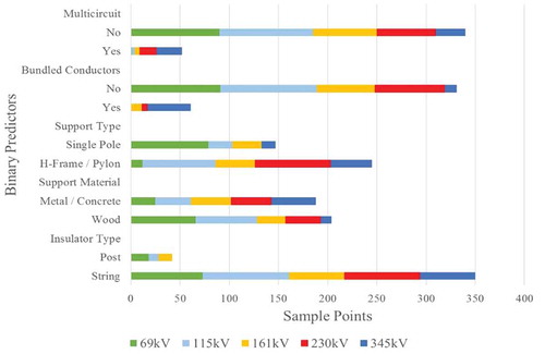
Signatures of voltage were less apparent among the binary predictors but visible, regardless. Most of the predictors displayed some distinctly lopsided classes, particularly for the lower and higher classes, as shown in Figure 7. The support type of the 69 kV class, for example, were mostly single poles, while the 115 kV class was mostly H-frames or pylons. Likewise, the 230 kV class was made up of exclusively H-frames or pylons. Similarly, bundled conductors were most commonly found in the 345 kV class, rarely in the 230 kV class, and never in the 69 kV and 115 kV classes. The 69 kV class was made up of mostly wooden supports, while the 345 kV class was mostly metal or concrete. Signatures in the middle classes were less distinct. For example, the 161 kV class fails to clearly stand out in any predictor. In the support type variable, the class was nearly split evenly. In the insulator type and multi-circuit variables, it resembled lower classes. In bundled conductors and support type variables, 161 kV displayed patterns similar to higher classes.

Figure 7. Bar chart of binary predictors symbolized by nominal voltage for sample points collected in this study.

3.3. Predictor performance

Out of all continuous predictors identified and collected, the height of transmission supports and span between supports were found to be the most effective for classifying voltage, followed by the spacing between conductors. Conductor spacing, support height, and support span were used as a primary variable for at least one partition in 29, 27, and 24 out of 30 model iterations, respectively, as shown in Table 3. These predictors also performed best in terms of their average variable importance rank, which is found in column two of Table 3. By this metric, support height and support span were most effective in the classification, followed by conductor spacing, with mean values of 3.55, 1.60, and 1.60, respectively. On the other hand, the right of way width performed the worst of the predictors. As shown by the “Null” mean variable importance rank, and 0 primary split shore, it was never used as a primary or surrogate variable, likely due to wide variation and numerous missing values.

Table 3. Predictor performance in tree construction over 30 iterations as shown by the count of tree where the predictor was use as a primary split and its mean variable importance rank (reprinted from Schmidt 2016, table 4).

	Total trees as primary split	Mean variable importance rank
Conductor spacing	29	3.55
Support height	27	1.60
Support span	24	1.60
Bundled conductors	15	4.18
Support type	14	4.10
Multi-circuit	1	6.12
Support material	0	6.25
Insulator type	0	6.71
Right of way	0	Null

Performance of the binary predictors was mixed. Bundled conductors and support type were used as primary splits in 15 and 14 trees out of 30, respectively. The only other binary predictor used as a primary variable was multi-circuit, and only once. The remaining variables were never used for a primary split, but they served as surrogate variables, as indicated by their mean variable importance ranks of 4.18 and 4.10, respectively. Based on these two metrics, bundled conductors and support type performed best among the binary predictors.

3.4. Classification accuracy

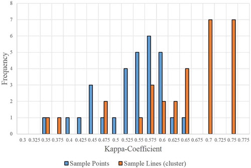
The tree-based classification used in this study yielded fair classification results. The mean predictive accuracy of the sample points classification after 30 iterations was 62.1%. The results varied greatly depending on how the samples were divided for testing and training, which is shown by the wide range of predictive accuracies in Table 4. The worst tree had a predictive accuracy of only 45.4% and the best tree, 70.9%. However, the overall distribution of the predictive accuracies was slightly negatively skewed by the 45.4% outlier, as Figure 8 suggests. The frequency plot shows that most of the trees produced predictive accuracies between 60% and 70%. While some trees yielded accuracies below 50%, the majority correctly classified 60% or more observations. The Kappa-coefficient showed a more conservative assessment of overall performance. Figure 9 shows a similar frequency plot of Kappa-coefficient for the 30 iterations. The mean Kappa-coefficient was 0.523, and most trees produced scored greater than 0.5.

Table 4. Summary classification statistics across 30 iterations, including prediction accuracy and Kappa for the sample points classification and sample lines (mode) classification, user accuracy and producer accuracy for each nominal voltage, and the number of primary splits (adapted from Schmidt 2016, table 6).

	Min.	Mean	Median	Std. Dev.	Max.
Prediction accuracy	45.4%	62.1%	64.3%	5.9%	70.9%
Kappa	0.332	0.523	0.536	0.069	0.632
Prediction accuracy (mode)	46.4%	70.1%	71.4%	8.4%	78.6%
Kappa (mode)	0.346	0.623	0.639	0.103	0.729
User accuracy
69 kV	0.396	0.682	0.679	0.146	0.962
115 kV	0.311	0.635	0.639	0.152	0.960
161 kV	0.000	0.483	0.471	0.179	1.000
230 kV	0.000	0.705	0.747	0.197	0.931
345 kV	0.282	0.665	0.697	0.203	1.000
Producer accuracy
69 kV	0.408	0.740	0.806	0.173	1.000
115 kV	0.286	0.620	0.639	0.176	0.898
161 kV	0.000	0.397	0.405	0.176	0.714
230 kV	0.000	0.684	0.750	0.230	1.000
345 kV	0.095	0.746	0.779	0.163	0.952
No. of primary Splits	3	5.9	6	1.5	8

Figure 8. Bar graph comparing the frequency of predictive accuracy for sample points and sample lines from 30 tree-based model iterations (adapted from Schmidt 2016, figure 5).

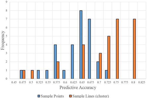
Figure 9. Bar graph comparing the frequency of Kappa-coefficient for sample points and sample lines from 30 tree-based model iterations (adapted from Schmidt 2016, figure 6).

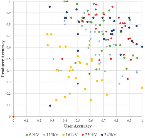
In testing, the producer and user accuracy of the each model vis-à-vis individual classes varied with each iteration, but the models consistently performed most poorly with respect to the 161 kV class. As evident by the clustering of yellow points in the middle of the graph in Figure 10, the 161 kV scores were consistently lower than those of other classes. Given the weak signatures of the 161 kV class compared to other classes, the trees had difficulty parsing it from other classes, particularly 115 kV and 230 kV, which negatively impacted their overall predictive accuracy. Thus, the trees developed in this study consistently yielded lower user and producer accuracies for that class, often mistakenly labeling observations as 161 kV and classifying 161 kV observations as other classes.

Figure 10. Scatter plot of producer and user accuracy results symbolized by nominal voltage from 30 tree-based model iterations. The random splitting process used to separate training and testing data resulted in underrepresented classes in some iterations, which accounts for outliers in the lower left of the plot (reprinted from Schmidt 2016, figure 7).

However, examination of the average classification rate showed that most misclassified observations were only one class higher or lower than the true class. Given the ordinal structure of voltage classes, the trees in this study performed better than the overall predictive, producer, and user accuracy suggests. In practice, a classification would not be performed with so few observations in the training dataset, as was the case for some trees included above. For this reason, trees with fewer than four sample lines, or 28 sample point observations, per class in the training dataset were excluded from the following tabulation. The confusion matrices of the remaining 17 trees were normalized by row, or actual class, and corresponding records across all matrices were summed, and then divided by 17 to produce the average classification rate for each class, as shown in Table 5. This table shows that on average the clear majority of observations were classified within one position of their true class. For example, an average of 0.966 69 kV observations, seen in the first row, were either classified as 69 kV or one class higher, 115 kV. On average, far fewer observations were classified as 161 kV, fewer as 230 kV, and even fewer, as 345 kV. This trend can be seen in all classes, wherein the classification rate declines in positions further from the true class, apart from the 161 kV class, which has a nearly even rate beyond the true class. Table 6, a confusion matrix from one of the best performing trees (shown in Figure 4), highlights a similar pattern.

Table 5. Two confusion matrices of average classification rate for select iterations where columns are predicted classes and rows are actual classes. The classification result for the sample points is on the left, and on the right, the result when aggregated to the sample lines where the class mode is identified for each line (adapted from Schmidt 2016, table 7).

	Sample points					Sample lines (mode)
	69 kV	115 kV	161 kV	230 kV	345 kV	69 kV	115 kV	161 kV	230 kV	345 kV
69 kV	0.791	0.175	0.023	0.009	0.001	0.858	0.142	0	0	0
115 kV	0.264	0.595	0.136	0.005	0	0.222	0.657	0.121	0	0
161 kV	0.162	0.192	0.393	0.116	0.136	0.157	0.201	0.422	0.102	0.118
230 kV	0	0.006	0.139	0.668	0.186	0	0	0.088	0.776	0.137
345 kV	0	0.002	0.04	0.179	0.779	0	0	0.029	0.088	0.882

Table 6. Two confusion matrices from one of the best models (as shown in Figure 4) where columns are predicted classes and rows are actual classes. The classification result of the sample points is on the left, and on the right, the final classification result where the mode from the sample points is identified for each line (adapted from Schmidt 2016, table 5).

	Sample points					Sample lines (mode)
	69 kV	115 kV	161 kV	230 kV	345 kV	69 kV	115 kV	161 kV	230 kV	345 kV
69 kV	44	5	0	0	0	7	0	0	0	0
115 kV	10	23	2	0	0	1	4	0	0	0
161 kV	9	11	20	2	0	2	1	3	0	0
230 kV	0	0	14	28	0	0	0	1	5	0
345 kV	0	0	3	8	17	0	0	0	1	3

Identifying the mode in the post-processing step significantly improved the overall performance of the final classification. As shown in Figure 11 example, identifying the mode, or most frequently predicted voltage from the sample points as the most likely voltage of the transmission line, smoothed over misclassifications and increased overall accuracy. The mean predictive accuracy of the sample lines classification after 30 iterations was 70.1%, as shown in Table 4. While the producer accuracy improved only slightly, the user accuracy increased greatly since many misclassified 161 kV sample points were smoothed over. Likewise, some misclassifications in the 69 kV, 115 kV, and 345 kV classes were smoothed over. Furthermore, the confusion matrices in Tables 5 and 6 show that misclassifications by more than one class position were reduced while misclassifications by more than two-class positions were eliminated. The distribution of orange bars in Figures 8 and 9 show that most trees had a predictive accuracy greater than 70% and up to 78.6% in the final classification – a significant improvement over the sample point classification.

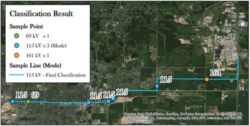
Figure 11. Large-scale map of the classification result from a single model (shown in Figure 4 and Figure 6) of one sample transmission line and its corresponding sample points. Five sample points were correctly classified as 115 kV, one as 69 kV, and one as 161 kV. Since the mode of the sample points is 115 kV, the final classification for the line shown is 115 kV.

3.5. Novelty, limitations, and future work

This study developed and tested a novel methodology to classify nominal transmission line voltage using predictor measurements taken from aerial imagery. Using the methods outlined in this study, predictors of voltage were successfully measured from aerial imagery using imagery interpretation and mensuration techniques. This methodology could be used to fill missing nominal voltage data, thereby improving the overall quality of geospatial electric power transmission datasets.

Despite its novelty, there are some key limitations to this methodology. While there is no other literature on nominal voltage classification with which to compare these results, the overall accuracy achieved in this study is considerably lower than classification results in other studies (Amancio et al. 2014; Pham et al. 2016; Torbick and Corbiere 2015). Likewise, the process of manually collecting predictor measurements from aerial imagery is time-intensive, which hinders the scalability of this methodology. These limitations provide opportunities for future work.

To improve the accuracy of this study, future work could be devoted to testing alternate classifiers, identifying additional predictors, and controlling the number of classes. Classifications trees were used in this study primarily for their transparency when compared to other classifiers, which was important for the purposes of this study given its foundational nature. However, more robust classifiers, such as support vector machines or neural networks could improve overall accuracy. Likewise, identifying and including additional predictors of nominal voltage could increase the overall predictive capacity of this method. Though this study identified predictors that were effective, there are likely other predictors that were not captured in this work. Other possible predictors, such as land cover or slope could be programmatically extracted using remote sensing techniques. Accuracy could also be improved by merging voltages into generalized classes, such as “below 100 kV,” “115–161 kV,” “230–287 kV,” etc. This approach would generate a less precise, more conservative estimate of nominal voltage, while still offering a degree of distinction between features in a geospatial transmission line dataset.

Furthermore, the scalability of this work is limited by the time-intensive nature of manually collecting predictor measurements from aerial imagery. As a result of this lengthy process, the sample size used for training and testing in this study was small, which in turn could have an impact on the overall accuracy of the results. To address this issue, future work could focus on leveraging non-imagery datasets to extract key predictors identified in this study. For example, collecting support span and support height measurements – the latter in particular – was time-intensive using the methods in this study. Capturing the support height predictor required imagery with precise metadata about date and time, which can be difficult to acquire. However, both predictors could hypothetically be extracted from vertical aeronautical obstruction data collected by the Federal Aviation Administration, since transmission line supports fall under this designation.

4. Conclusion

This paper presents a foundational methodology that draws knowledge from the electric power systems, remote sensing, and machine learning disciplines to address a significant problem in open geospatial datasets of US electric power transmission lines – missing nominal voltage data. Of all predictors examined in this study, we found that support height, span, and conductor spacing are the strongest predictors of nominal voltage. By leveraging these predictors in a tree-based supervised classification, nominal voltage can be reliably classified within one voltage class for four out of the five classes in this study. We have developed an open source, data-driven, and repeatable methodology to address the problem of missing voltage data in an effort to improve a historically restricted, valuable dataset for research and analysis.

Notice of copyright

This manuscript has been authored by UT-Battelle, LLC under Contract No. DE-AC05-00OR22725 with the U.S. Department of Energy. The United States Government retains and the publisher, by accepting the article for publication, acknowledges that the United States Government retains a non-exclusive, paid-up, irrevocable, worldwide license to publish or reproduce the published form of this manuscript, or allow others to do so, for United States Government purposes. The Department of Energy will provide public access to these results of federally sponsored research in accordance with the DOE Public Access Plan (http://energy.gov/downloads/doe-public-access-plan).

Acknowledgements

Content, Tables, and Figures in this paper were derived, in part, from the primary author’s master’s thesis (Schmidt 2016). The authors thank Olufemi A. Omitaomu for his constructive suggestions and assistance in finalizing this manuscript.

Disclosure statement

No potential conflict of interest was reported by the authors.

Additional information

Funding

This research was sponsored by the U.S. Department of Defense at U.S. Department of Energy's (DOE) Oak Ridge National Laboratory, under DOE contract number DE-AC05-00OR22725.

References

- Amancio, D. R., C. H. Comin, D. Casanova, G. Travieso, O. M. Bruno, F. A. Rodrigues, and L. F. Costa. 2014. “A Systematic Comparison of Supervised Classifiers.” PLos ONE 9 (4): e94137. doi:10.1371/journal.pone.0094137.
- Ambite, J. L., Y. Arens, E. Hovy, A. Philpot, L. Gravano, V. Hatzivassiloglou, and J. Klavans. 2001. “Simplifying Data Access: The Energy Data Collection Project.” Computer 34 (2): 47–54. doi:10.1109/2.901167.
- Central Station Engineers of the Westinghouse Electric Corporation (CSEWEC). 1964. Electrical Transmission and Distribution Reference Book. West Pittsburgh, PA: Westinghouse Electric Corporation.
- Donker, F. W., B. van Loenen, and A. K. Bregt. 2016. “Open Data and Beyond.” International Journal of Geo-Information 5 (4): 48. doi:10.3390/ijgi5040048.
- Goodchild, M. F., and J. A. Glennon. 2010. “Crowdsourcing Geographic Information for Disaster Response: A Research Frontier.” International Journal of Digital Earth 3 (3): 231–241. doi:10.1080/17538941003759255.
- Hong, H., B. Pradhan, X. Chong, and D. T. Bui. 2015. “Spatial Prediction of Landslide Hazard at the Yihuang Area (China) Using Two-Class Kernel Logistic Regression, Alternating Decision Tree and Support Vector Machines.” Catena 133: 266–281. doi:10.1016/j.catena.2015.05.019.
- James, G., D. Witten, T. Hastie, and R. Tibshirani. 2013. An Introduction to Statistical Learning with Applications in R. New York: Springer.
- Janssen, M., Y. Charalabidis, and A. Zuiderwijk. 2012. “Benefits, Adoption Barriers and Myths of Open Data and Open Government.” Information Systems Management 29 (4): 258–268. doi:10.1080/10580530.2012.716740.
- Kerski, J. J., and J. Clark. 2012. The GIS Guide to Public Domain Data. Redlands: ESRI Press.
- Kirtley, J. L. 2010. Electric Power Principles: Sources, Conversion, Distribution and Use. West Sussex: John Wiley and Sons.
- Li, M., J. Im, and C. Beier. 2013. “Machine Learning Approaches for Forest Classification and Change Analysis Using Multi-Temporal Landsat TM Images over Huntington Wildlife Forest.” GIScience and Remote Sensing 50: 361–384.
- Minnesota Geospatial Information Office. 2014. “Electric Transmission Lines and Substations, 60 Kilovolt and Greater, Minnesota.” Accessed 25 September 2014. https://catalog.data.gov/dataset/electric-transmission-lines-and-substations-60-kilovolt-and-greater-minnesota-2014.
- Murray-Rust, P. 2008. “Open Data in Science.” Serials Review 34 (1): 52–64. doi:10.1016/j.serrev.2008.01.001.
- Oak Ridge National Laboratory Geographic Information Science and Technology Group, Los Alamos National Laboratory, Idaho National Laboratory, National Geospatial-Intelligence Agency, Homeland Security Infrastructure Program Team. 2017. “Electric Power Transmission Lines.” (dataset). Homeland Infrastructure Foundation-Level Data Open. Accessed 5 February 2018. https://hifld-geoplatform.opendata.arcgis.com/datasets/electric-power-transmission-lines.
- Pham, B. T., D. Tien Bui, M. B. Dholakia, I. Prakash, and H. V. Pham. 2016. “A Comparative Study of Least Square Support Vector Machines and Multiclass Alternating Decision Trees for Spatial Prediction of Rainfall-Induced Landslides in A Tropical Cyclones Area.” Geotechnical and Geological Engineering 34 (6): 1807–1824. doi:10.1007/s10706-016-9990-0.
- Quinlan, J. R. 1986. “Induction of Decision Trees.” Machine Learning 1 (1): 81–106. doi:10.1007/BF00116251.
- Rustebakke, H. M., ed. 1983. Electric Utility Systems and Practices. 4th ed. New York: John Wiley & Sons.
- Schmidt, E. H. 2016. “Classifying Nominal Voltage of Electric Power Transmission Lines Using Remotely-Sensed Data.” Master’s Thesis, University of Tennessee. http://trace.tennessee.edu/utk_gradthes/3807
- Shoemaker, T. M., and J. E. Mack. 2002. The Lineman’s and Cableman’s Handbook. 10th ed. New York: McGraw-Hill Companies.
- Short, T. A. 2004. Electric Power Distribution Handbook. Boca Raton, FL: CRC Press.
- Simpson-Porco, J. W., F. Dörfler, and F. Bullo. 2016. “Voltage Collapse in Complex Power Grids.” Nature Communications 7. doi:10.1038/ncomms10790.
- Singh, K. K., J. B. Vogler, D. A. Shoemaker, and R. K. Meentemeyer. 2012. “LiDAR-Landsat Data Fusion for Large-Area Assessment of Urban Land Cover: Balancing Spatial Resolution, Data Volume and Mapping Accuracy.” ISPRS Journal of Photogrammetry and Remote Sensing 74: 110–121. doi:10.1016/j.isprsjprs.2012.09.009.
- Therneau, T. M., and E. J. Atkinson. 2017. “An Introduction to Recursive Partitioning Using the RPART Routines.” Cran.R-Project. Accessed 12 March. https://cran.r-project.org/web/packages/rpart/vignettes/longintro.pdf.
- Torbick and Corbiere. 2015. “Mapping Urban Sprawl and Impervious Surfaces in the Northeast United States for the past Four Decades.” GIScience and Remote Sensing 52: 746–764. doi:10.1080/15481603.2015.1076561.
- Wang, W., and M. Barnes. 2014. “Power Flow Algorithms for Multi-Terminal VSC-HVDC WithDroop Control.” IEEE Transactions on Power Systems 29 (4): 1721–1730. doi:10.1109/TPWRS.2013.2294198.