Estimation of soil moisture using deep learning based on satellite data: a case study of South Korea

Abstract

The Korea Meteorological Administration uses soil moisture (SM) observed by the Advanced Microwave Scanning Radiometer-2 (AMSR2) to monitor drought. However, it may not be appropriate for monitoring drought in South Korea due to significant underestimation of SM. In this study, we used a deep learning method that performs better than traditional statistical and physical models for reliable estimation of SM based on remotely sensed satellite data. For estimating SM, we carefully selected input variables that exhibit a feedback loop with SM. To build an effective deep learning model, we examined the influences of sampling criteria and input parameters as well as the accuracy of several deep neural networks. The selected model was cross-validated to determine its stability. The estimated SM using deep learning had a high correlation coefficient (R) of 0.89 and a low root mean square error (RMSE; 3.825%) and bias (−0.039%) compared to in-situ measurements. A time series analysis using dynamic time warping was conducted which showed that the estimated SM was almost similar to the in-situ SM. In order to investigate the improvement in SM estimation using our method, it was compared with the Global Land Data Assimilation System and AMSR2. Significant improvements in R and a reduction in error values by more than half were achieved using our method. The estimated SM has finer spatial resolution at 4 km, and it can be rapidly produced, which will be useful for drought monitoring over the Korean Peninsula in near-real-time.

Keywords:

• soil moisture
• deep learning
• South Korea
• dynamic time warping

1. Introduction

Soil moisture (SM) influences vegetation growth and weather by controlling the heat and water budget between the surface and atmosphere (Srivastava et al. 2013a; Jiang and Weng 2016; Lee et al. 2017) and directly affects the exchange of trace gases on land (Seneviratne et al. 2010). SM is an indicator of water stress for vegetation and is used for monitoring agricultural drought (Bolten et al. 2010; Mao et al. 2017; Padhee et al. 2017). There are various means of observing surface SM, such as in-situ measurement by gravimetric or time domain reflectometers, remote sensing by satellites, and land-surface or hydrologic modelling (Bi et al. 2016). In-situ measurements can directly obtain steady and accurate values of SM but cannot represent a large area spatially. Furthermore, these ground measurements consume time and labour, and it is expensive to maintain both the quality and dense network of the observations (Chang and Islam 2000; Elshorbagy and Parasuraman 2008). Numerical models can regularly simulate SM at global or local scales but have limits associated with the uncertainty of complex calculations, coarse spatial resolutions for local areas, and excessive calculation times. Microwave remote sensing also provides SM observations by using large differences between the wet and dry soil dielectric properties with spatial consistency over a large area (Liang, Li, and Wang 2012). Microwave sensors can observe the surface under all weather conditions, including in the rain or with clouds. These have narrow spatial-temporal coverage and spatial resolution for a specific local area. Vegetation is a major disturbance for detecting signals of stored water within soil because vegetation attenuates soil emissions and adds its own emissions to the microwave signal (Liou, Liu, and Wang 2001). To avoid the effects of vegetation, low microwave frequencies (L-band, 1–2 GHz) have been used to measure SM, but they are affected by radio frequency interference over Northeast Asia (Oliva et al. 2012; Lee et al. 2017).

To monitor drought over the Korean Peninsula, the Korea Meteorological Administration (KMA) has used the Japan Aerospace Exploration Agency (JAXA) algorithm (Koike 2013) based on the Advanced Microwave Scanning Radiometer-2 (AMSR2) SM level 3 product with a three-day delay in delivery time and 0.1° resolution, averaged by a daily and seven-day moving window to reduce noise and missing areas of data. However, the AMSR2 SM still has low correlations with in-situ SM and significantly underestimates trends over the Korean Peninsula compared to in-situ observations during all observation periods (Cho, Moon, and Choi 2015; Lee et al. 2017). These differences make it difficult to use this method for reliable drought monitoring. Moreover, AMSR2 has a coarse spatial resolution (greater than 10 km) and uncertainty in near-shore areas, similar to other microwave sensors.

Deep learning is a machine learning method that has shown better performance compared to other traditional statistical and physical methods to estimate surface parameters such as soil moisture, evapotranspiration, leaf area index, and solar insolation (Liou, Liu, and Wang 2001; Elshorbagy and Parasuraman 2008; Yeom and Han 2010; Menzies et al. 2013; Yeom et al. 2015). Machine learning methods, such as support vector machines (SVMs), random forest (RF), and artificial neural networks (ANNs), have been applied in many studies. Studies involving SM based on remote sensing have been conducted by down-scaling the established SM or using improved accuracy based on data from microwave sensors (Liou, Liu, and Wang 2001; Ahmad, Kalra, and Stephen 2010; Srivastava et al. 2013b; Rodrigues-Fernandez et al. 2015; Im et al. 2016; Ma and Liu 2016). Furthermore, deep learning has advanced significantly based on ANNs and has the capacity to process complex input data and learning tasks (Ali et al. 2015).

Our goal in this study is to enable rapid, reliable, and spatially detailed drought monitoring by replacing AMSR2 SM with daily estimates of SM through deep learning with a 4-km spatial resolution on the Korean Peninsula. In addition, we use only level 2 products so that our method for estimating SM can be easily adapted to other satellites. Using input variables with hourly intervals for our study helps to estimate SM at finer temporal resolutions to identify diurnal variations that would be helpful in improving the performance of land-surface models (Song, Gua, and Zhang 2009).

2. Materials for deep learning and spatial-temporal coverage

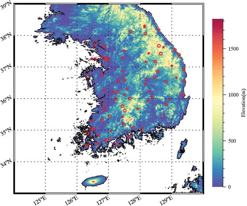
Figure 1 indicates the study area with elevation information and the location of in-situ measurements (stars and pentagon symbols in red, respectively). As shown in Figure 1, over 70% of the Korean Peninsula consists of mountainous areas. The temporal period was set from 2014 to 2016, and we excluded data in certain periods, such as in winter and early spring (from January to March and from November to December). The weather on the Korean Peninsula during winter is so cold and dry that stored water is frozen within the soil layer. This makes it difficult to obtain accurate soil moisture readings through ground-based observations. The characteristics of the material used for deep learning are summarized in Table 1.

Table 1. Summary of materials used.

Parameter	Sensor	Resolution (spatial/temporal)	Pre-process	Reference
Outgoing Longwave Radiation (OLR)	COMS/MI	4 km/15 min	Calculating daily min/max/mean	Inoue and Ackerman (2002)
Insolation (INS)	COMS/MI	4 km/15 min	Calculating daily min/max/mean	Kawamura, Tanahashi, and Takahashi (1998)
Accumulated Precipitation for 12 h (Pr12h)	Rain gauge of AWS	Point/10 min	IDW Interpolation with 12-km moving window at 4-km resolution
Accumulated Precipitation for 24 h (Pr24h)	Rain gauge of AWS	Point/10 min	IDW Interpolation with 12-km moving window at 4-km resolution
Albedo (Al)	MODIS	0.05°/daily	Nearest neighbourhood interpolation for 4-km grid	Strahler et al. (1999b)
Normalized Difference Vegetation Index (NDVI)	MODIS	500 m/16 days	Low peak correction and spline interpolation to daily	Didan et al. (2015)
2-m air temperature (Ta)	Thermometer of AWS	Point/10 min	Kriging interpolation at 4-km resolution, daily min/max/mean/standard deviation
2-m relative humidity (Hm)	Hygrometer of AWS	Point/10 min	Kriging interpolation at 4-km resolution, daily min/max/mean/standard deviation
Yearly land cover (LC)	MODIS	500 m/year	Calculating land-cover fraction according to four modified land types (high density, low density, crop, urban and barren) within a 4-km grid	Strahler et al. (1999a)
Topology (DEM, Slope)		1 km	Calculating mean, standard deviation, and nearest value within 4-km grid
Precipitation of IMERG	Multi-sensors including MW, IR	0.1°/d	Nearest neighbourhood interpolation on a 4-km grid	Huffman et al. (2017)
GLDAS (Noah)		0.25°/3 h	Calculating daily mean	Rodell et al. (2004)
AMSR2 (JAXA)	GCOM-W1/AMSR2	0.1°/twice per day	Calculating daily mean	Fujii, Koike, and Imaoka (2009)
Soil moisture	CS615/CS616	10 cm depth/10 min		Scientific (1996) Scientific (2016)

Figure 1. Elevation map of South Korea and the location of soil moisture in-situ observations (star: target observation site, pentagon: excluding observation site).

2.1. Input satellite data

Naturally, SM is influenced by energy, mass flux, and the effects of vegetation. Therefore, we collected various surface and thermal variables from satellites, such as solar insolation (INS), outgoing longwave radiation (OLR), broadband albedo (AL), normalized difference vegetation index (NDVI), and the integrated multi-satellite retrievals for global precipitation measurement (IMERG). The INS and OLR products were obtained from the Communication, Ocean, and Meteorological Satellite (COMS)/Meteorological Imager (MI) of KMA, calculated by a modified physical model (Kawamura, Tanahashi, and Takahashi 1998) and a split-window method (Inoue and Ackerman 2002), respectively. NDVI, land cover (LC), and AL were provided by the moderate-resolution imaging spectroradiometer (MODIS). NDVI reflects the vitality of vegetation, but it cannot provide any information on LC and vegetation type, such as crop, forest, grass, etc. We also used LC because it influences SM along with vegetation type (Crow et al. 2012; Petropoulos 2013).

NDVI (MOD13A1) was obtained as the maximum value composite (MVC) during a 16-day period with a 500-m resolution that reduced the missing area and minimized the bi-direction reflectance distribution function (BRDF) effects (Didan et al. 2015). The MODIS albedo product (MCD43C3) provided seven spectral and three broadband albedos, and we used three broadband albedos (vis 0.3–0.7 µm, near-infrared 0.7–5.0 µm, and total shortwave 0.3–5.0 µm) to consider the solar energy absorbed into the canopy. These broadband albedos, which represent the ratio of incident solar radiation to the radiation reflected by the Earth’s surface, were calculated using the following procedures: atmospheric correction, BRDF modelling, and narrow-to-broadband conversion (Strahler et al. 1999b).

IMERG precipitation was developed to compensate for the lack of spatial-temporal coverage of single low-Earth-orbit satellites by adding all available satellites that include geosynchronous-Earth-orbit IR sensors. The IMERG algorithm can be briefly described by the following procedures: 1) inter-calibration of the microwave estimate, 2) Lagrangian time interpolation and Kalman filtering, 3) filling of “holes” in the passive microwave constellation using microwave-calibrated IR estimates, and 4) controlling bias by incorporating gauge data for post-research (Huffman et al. 2017). From the various temporal resolutions, such as 30 min, 3 h, daily, and monthly IMERG, we selected daily precipitation to consider the daily SM. IMERG has various versions, such as early, late, and final runs, with different latencies of 6 h, 18 h, and 4 months, respectively. We used the late-run version to estimate SM for a near-real-time operation that adopted forward and backward morphing to be suitable for daily and longer composite period applications (Huffman, Bolvin, and Nelkin 2017).

2.2. In-situ measurement and auxiliary data

To train and validate, we also collected ground measurement observations from the Rural Development Administration (RDA) of Korea. Since 2000, the RDA has observed SM at the near-surface level (~10 cm depth) and operates 72 observation sites throughout the Korean Peninsula. The in-situ SM has been measured using SM probes having accuracies of ±3 and 2.5% (Scientific 1996, 2016). Precipitation is crucial as a major source of stored water in soil layers; therefore, we collected 12-h and 24-h accumulated precipitation (mm/12 h or 24 h) data from Automatic Weather System (AWS) measurements operated by the KMA. Since precipitation penetrates the soil and is stored between soil particles for several days, we used precipitation data from seven days before the present day (Lee et al. 2017). This also applied to the IMERG data. The 2-m air temperature (Ta) and relative humidity (Hm) observed by the AWS were also collected because they affect SM through transpiration between the surface and atmosphere. Currently, the AWS has observed climatic variables at 10-min intervals at 692 sites. The measurements of the AWS were added to establish the reference accuracy and were removed or replaced by other satellite products.

Elevation and slope information from the Global 30 Arc-Second Elevation (GTOP30) of the USGS with 1-km resolution was collected because these variables influence SM content through infiltration, runoff, and drainage (Giraldo, Madden, and Bosch 2013; Petropoulos 2013).

2.3. Soil moisture observed by GLDAS and AMSR2

The Global Land Data Assimilation System (GLDAS) was developed jointly by the National Aeronautics and Space Administration (NASA) Goddard Space Flight Center (GSFC) and the National Oceanic and Atmospheric Administration (NOAA) National Centers for Environmental Prediction (NCEP) (Rodell et al. 2004). GLDAS yields various surface parameters, including soil properties, heat fluxes, snow properties, canopy conductance, and transpiration, by forcing a land-surface model using nine observation networks and several data assimilation techniques (Rodell et al. 2004). It was used as a reference to validate or train the status of land and water/energy flux variables because of its relatively high stability and accuracy compared to the assessment of SM by satellite (Park and Choi 2014; Cho, Moon, and Choi 2015; Bi et al. 2016; Fang et al. 2016; Lee et al. 2017). GLDAS provides SM using models (Noah, Mosaic, Variable Infiltration Capacity, and the community land model) and has a 1° resolution, except for when using the Noah model (0.25°). According to Bi et al. (2016), four models captured the temporal variation well compared with in-situ SM measurements, and Noah has the second-highest performance with a high R (greater than 0.57) and low RMSE (less than 0.169 m³/m³). We used the SM from Noah because it has the finest spatial resolution.

AMSR2 is onboard the Global Change Observation Mission (GCOM-W1) to observe water cycles and provides a variety of information on water flux, such as integrated water vapor, sea surface temperature, sea surface wind speed, snow depth, and SM, as it ascends to a crossing time of 13:30 local time (JAXA 2013). It employs a look-up table method from a brightness temperature of 10 and 36 GHz (Fujii, Koike, and Imaoka 2009). This algorithm adopts MODIS NDVI to consider the water content of vegetation, which influences the remotely sensed observations of microwave sensors. According to AMSR2 validation results (Kaichi et al. 2013), the SM of AMSR2 has a release accuracy of ±10%, but it shows lower accuracy on the Korean Peninsula (Lee et al. 2017). The SM values from GLDAS and AMSR2 were used as comparisons to assess the performance of the deep learning model developed herein.

3. Methodology

3.1. Pre-processing of input data

First, we removed several in-situ measurements according to the surrounding environment when the ground station was located in the middle of an urban area or when a river, lake, or reservoir was within a 2-km radius. Urban areas have unnatural SM due to artificial surfaces and rain drainage facilities. Since most satellite data have spatial resolutions greater than a few kilometres, the presence of water resources such as rivers, streams, or reservoirs near the observation site may cause errors in estimating SM. After this filtering, more than half of the station data were excluded. Then, 33 stations were selected to train the deep learning model.

We unified all satellite data to the same projection and spatial resolution as a cylindrical (equirectangular) map projection with a 4-km resolution. To reduce the difference by distance between the location of each AWS and RDA station, we converted the daily precipitation, Ta, and Hm to a grid format. Ta and Hm were gridded using kriging interpolation; however, precipitation data were calculated using the inverse distance weighting (IDW) method within the 12.5-km moving window used by the AMSR2 correction (Lee et al. 2017). The kriging method gave better results for the interpolation of air temperature, as reported by Li, Cheng, and Lu (2005) and Mahdian et al. (2009). Nguyen et al. (2015) also interpolated Ta and Hm using a kriging method with low error (RMSE: 2.195% and 7.155%, respectively). In this study, we validated interpolated variables using 10% of the total observations that were randomly selected. As a result of the validation, Ta was 1.392°C, Hm was 8.217%, and the 12-h and 24-h precipitation had RMSE values of 3.83 mm/12 h and 10.64 mm/24 h respectively. The precipitation fluctuated more than Ta and Hm did and could not be detected under 0.1 mm due to rain gauge limitations. Furthermore, non-physical negative precipitation values were calculated in clear areas (non-precipitation areas) due to the nature of the kriging method that produced spatially continuous values.

Products, such as OLR and INS from COMS/MI, were used to calculate the daily minimum, maximum, and average to consider the variations in the energy flux. There were significant altitude differences within the 4-km grid, because the Korean Peninsula is mountainous, as shown in Figure 1. Therefore, the topology data, such as the digital elevation model (DEM) and slope, were calculated by the average, standard deviation, and nearest value within the 4-km grid, to include input variables.

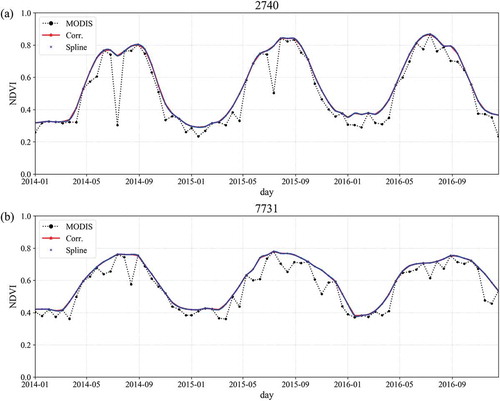
Although the MVC was used to avoid error, the NDVI product still had a low peak problem, a rapid decrease in index, and short recovery in vegetation (black dashed line with a circle in Figure 2). We corrected NDVI to assess the water stress of vegetation indirectly. If the low peaks could not be corrected, incorrect signals regarding the vegetation were entered, and the error would increase. In addition, identical values were used for 16 days; therefore, the variation in vegetation status was not considered in the SM estimate. To correct this noise, we used an iteration of the multinomial regression referred to by Yeom, Han, and Kim (2006). This method selected higher values between the original NDVI value and the simulated value by multinomial regression to correct for noise. The corrected NDVI was converted from 16-day to daily NDVI using spline interpolation. Figure 2 provides the time series graphs of MODIS NDVIs, corrected by multinomial regression and interpolated by a spline. According to the results from the correction and the interpolation to daily values, the corrected NDVI (red line in Figure 2) was reconstructed well by correcting the low peaks of MODIS NDVI. The daily interpolated NDVI (blue point in Figure 2) simulated smoothly the temporal changes between the 16-day intervals.

Figure 2. Comparison of temporal variations between MODIS (black circle), corrected (red solid), and daily interpolated (blue point) NDVI at Stations 2740 and 7731 during 2014 to 2016.

The LC has been calculated using a variety of variables, such as enhanced vegetation index, surface temperature, and adjusted reflectance, but there is still a significant difference when compared to the results of field-based surveys (Cho et al. 2014). Therefore, we modified the existing land type in the study area from the original 16 types of land cover to four simple categories: “high density” (evergreen broadleaf forest, evergreen needleleaf forest, deciduous broadleaf forest, deciduous needleleaf forest, and mixed forest); “low density” (closed shrub, open shrub, savannas, grass); “crop;” and “urban and barren.” We then calculated the fractional coverage according to each modified land type to consider its effect.

3.2. Configuration of the deep neural network

Deep learning is a machine learning method that emulates the decision making of the human brain. In this study, the H2O package of the R studio was used for building an SM estimation model by using remotely sensed satellite data. The deep learning of H2O is a supervised learning method with a feed forward network and error back propagation. Therefore, it needs a true value to calculate errors, which are used to control the weighting of each node in the hidden layers. The deep neural network consists of one input layer, a response variable (in-situ SM by RDA), several hidden layers with a number of nodes, and an output variable (estimated SM by deep learning), as in Zhang et al. (2017). We set the default deep neural network as 3-hidden-layer, 300-node, and 3000-epoch with the “Rectifier” function among the six activation functions as follows: “Tanh,” “TanhWithDropout,” “Rectifier,” “RectifierWithDropout,” “Maxout,” and “MaxoutWithDropout.” The “Rectifier” activation function has become widely used in deep learning models and is able to accelerate the convergence of the stochastic gradient descent because “Rectifier” is a non-saturating nonlinearity function (Nair and Hinton 2010; Krizhevsky, Sutskever, and Hinton 2012). Conversely, the traditional “sigmoid” or “Tanh” function easily saturates, slowing the training procedure when applied to deep neural networks. To select input variables, we examined the accuracy of the trained model by removing several input variables with a default deep neural network. Various deep neural networks were examined for accuracy to identify the optimal deep neural network structure. As in prior analyses, the selected model was evaluated by cross-validation (k-folds) to examine its stability. The k-folds randomly divided a whole dataset into n parts, and each part was then assigned as a validation or training dataset. For example, 3-folds divided an entire dataset into three parts. The first two parts were assigned as training, and the other was used to validate. Next, the middle part was assigned as training, and the others were used to validate. Finally, the first part was assigned as training, and the others were used to validate. If the n-number was large, the model was more stable and needed a longer calculation time.

3.3. Similarity measure of soil moisture time series using dynamic time warping

Dynamic time warping (DTW) is a method for measuring the similarity of data from two different time series and was introduced for comparing speech recognition by Sakoe and Chiba (1978). DTW can be applied to diverse remote-sensing research studies, such as change detection, classification of LC, and analysis of the similarity of trajectories (Petitjean, Inglada, and Gancarski 2012; Guan et al. 2016; Sharif and Alesheikh 2017). The method used for DTW followed the procedure given by various researchers (Muller 2007; Jeong, Jeong, and Omitaomu 2011; Guan et al. 2016). We assumed that we have two different time series datasets, such as A with length m and B with length n. First, we created a distance matrix D with an array. The D matrix was composed of as each element. Then, an accumulated cost matrix D_ac was calculated using the D matrix in the following Equation (1):

(1)

Second, a warping path was determined by calculating Equation (2) based on D_ac as follows:

(2)

Establishment of the optimal warping path needed to satisfy three conditions:

• Boundary condition: and .

• Monotonicity condition: and .

• Step-size condition: for .

The determined warping path represented the DTW distance between time series A and B. In this study, we compared the similarity of each SM using deep learning, AMSR2, and the GLDAS time series to in-situ measurements.

4. Results and analysis

4.1. Analysis of sampling criteria

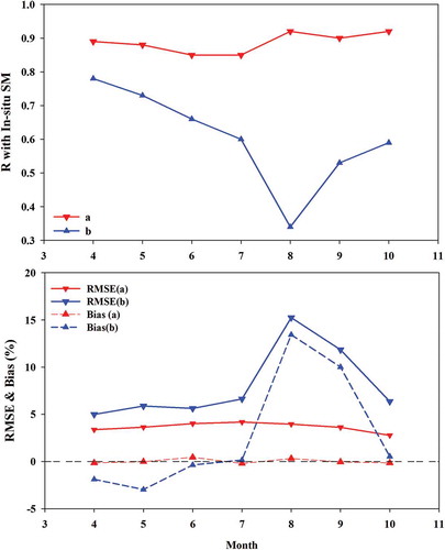
The collected dataset was divided into two categories: training and validation. First, we divided the dataset according to year: the first two years were assigned to training, and the last year was assigned to validation. Next, we divided the dataset through random selection with a ratio of 75% training and 25% validation. The former was strictly a dividing method and was more suitable for operational purposes than the latter. A well-built model does not require an additional training procedure due to it perfectly dividing the validation and training datasets. The latter method has an advantage in that it can reflect the characteristics of a whole dataset because it samples by order during the entire period. However, the model may need training to reflect changes in the environment. Figure 3 shows the scatter and density plots of each trained model by the sampling method. The trained model by percentage sampling (Figure 3(b,d)) had higher correlation coefficients (R) for the in-situ measurements and lower RMSE and bias than the trained model by yearly sampling (Figure 3(a,c)). We examined the variations in R, RMSE, and bias by month (Figure 4). The estimated SM by percentage sampling showed a steady, high R and low error value. In contrast, the SM using annual sampling tended to fluctuate unstably with the R and error values by month.

Figure 3. Scatter (a, b) and density (c, d) plots of estimated SM using deep learning according to two samplings (a, c: yearly/b, d: percentage).

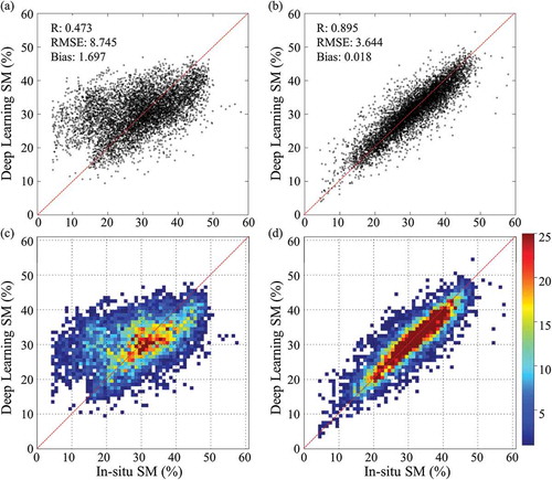
Figure 4. Variations in R, RMSE, and bias according to month (a: percentage sampling, b: yearly sampling).

To identify the cause of the errors, we selected time series data by annual sampling in accordance with the two stations that show the lowest R (Station 6732: 0.08; Station 7731: −0.04) and the highest RMSE (Station 6732: 9.803%; Station 7731: 9.542%) values compared with the in-situ SM. In Figure 5 (a,b), both time series plots had similar difference trends that dramatically increased during the summer. In-situ SM during August and September decreased, while the estimated SM by annual sampling increased as often as precipitation occurred. As shown in Figure 5 (c–e), the average daily precipitation in August steadily decreased over three years. In addition, unlike in 2014, the spatial distribution in 2016 is non-smooth and discontinuous. These graphs demonstrated changes in the precipitation pattern where precipitation occurred more commonly in a small area. Interpolated daily precipitation of the AWS was not sufficient to reflect this recently changing pattern of precipitation because AWS precipitation was interpolated by a 12-km moving window that referred to the mean distance between AWS sites. Therefore, we selected the percentage sampling method for the entire period.

4.2. Training parameters analysis

In total, 62 types of input parameters were selected to train the deep learning model to estimate SM. We tested the accuracy of each model, which was trained by excluding several parameters (Table 2). Overall, the entire trained model showed a high R (greater than 0.87) and a low RMSE (less than 4.15%). When removing NDVI, DEM and slope (topography), and LC fraction, the accuracy of the trained models decreased slightly. At all stages of parameter removal, the accuracy of the training model was slightly reduced. The decrease in accuracy was largest when precipitation was excluded from the input parameters. These results indicated that precipitation was a major parameter for estimating SM. Topography and surface status, such as NDVI and LC fractions, were also major influencers for SM. The columns in Table 2, indicated as 0.1 and 0.2 dropped nodes, tested the accuracy of the trained model by randomly dropping 10% and 20%, respectively, of the nodes of each hidden layer using the “RectifierWithDropout” activation function. Some parameters, such as OLR, AL, and Hm, had little influence on the accuracy of training the model even after the removal stage. Both trained models with randomly dropped nodes showed almost similar accuracy as the prototype. These results were likely due to the appropriate selection of input parameters to estimate SM. When Ta and Hm were removed, there was less change in the accuracy than expected. The observation net for interpolation was spatially inhomogeneous and was influenced by errors. According to Ryu, Han, and Park (2013), the accuracy of reanalysis Ta based on in-situ measurements fluctuated according to the variation in elevation. The decrease in accuracy was not significant even when precipitation was removed, likely due to the uncertainty of interpolation, similar to that for Ta and Hm, notwithstanding the superiority of deep learning.

Table 2. The accuracy summary of each trained deep learning model by 1st removing variables.

Removing variables	None	OLR	INS	AL	NDVI	AWS precipitation	AWS Ta	AWS Hm	Dem, Slope	Land-cover fraction	0.1 drop	0.2 drop
R	0.89	0.89	0.88	0.89	0.88	0.87	0.88	0.89	0.87	0.87	0.89	0.89
RMSE (%)	3.644	3.893	3.958	3.854	4.019	4.233	4.088	3.933	4.050	4.150	3.834	3.912
Bias (%)	0.018	−0.245	0.002	−0.039	−0.310	−0.062	−0.479	−0.078	0.055	0.112	−0.570	−0.585

As mentioned in the Introduction, one goal of this study was estimating SM using only satellite products. We therefore examined the accuracy of the trained models, with the exception of Ta and Hm, with the remaining variables removed one-by-one (Table 3). According to the results of this examination, the accuracy of the training model repeats the pattern of incrementing and decrementing each time the variable was removed. Unlike the previous analysis, when Ta and Hm were removed together, the accuracy tended to decrease, and other variables showed similar trends. When only one variable was removed, the effect of the removal was compensated for by the other variables, but when multiple variables were removed, there was decreased accuracy. When removing satellite variables (when AL, INS, and OLR are removed together), the accuracy tended to be slightly higher than when just AL and INS were removed. These results may have been a result of the absence of input or output energy information. INS represented incoming solar radiation, OLR provided emitted radiation by the surface (longwave), and AL indicated reflected solar energy by the surface (shortwave). Removing just the incoming or outgoing energy flux resulted in lower accuracy than when all information regarding the energy flux was removed due to the disturbance of the energy balance. The 0.1 and 0.2 dropped nodes in Table 3 were calculated through a process similar to that used to obtain the values in Table 2, and the Ta and Hm were removed before the random drop. The accuracy of the randomly dropped models was slightly reduced compared to the prototype. This indicated that the selection of the input variables had a similar accuracy when compared to that of the random drop. As the result of input parameter analysis, AL, INS, and OLR were included as energy flux parameters in the trained model. Lastly, accumulated precipitation for 12 and 24 h of the AWS were replaced by IMERG daily accumulated precipitation to result in the use of satellite data only. Finally, AL, INS, OLR, NDVI, topology, and IMERG precipitation (in total, 38 types of parameters) were selected for the trained model, which had similar accuracy (R: 0.87, RMSE: 4.102, bias: 0.064) compared to the trained model that excluded only Ta and Hm.

Table 3. The accuracy summary of each trained deep learning model by 2nd removing variables.

Removing Variables	None	Ta, Hm	AL, Ta, Hm	AL, Ta, Hm, INS	AL, Ta, Hm, INS, OLR	0.1 drop	0.2 drop
R	0.89	0.88	0.87	0.85	0.86	0.88	0.87
RMSE (%)	3.644	3.937	4.189	4.401	4.274	3.958	4.093
Bias (%)	0.018	0.113	−0.220	−0.057	−0.037	−0.123	−0.359

4.3. Analysis of a deep neural network to select an optimal structure

It was important to determine the number of hidden layers and nodes for the optimal structure of the neural network because the structure of a deep neural network influences the accuracy and time for training. Therefore, we selected the number of hidden layers and nodes using a comparison between several structures of the deep neural network. Early-stopping was applied to avoid over-fitting the training data and to reduce meaningless training time. We established a threshold of 0.5% Mean Squared Error (MSE),) and determined the last three averages and the prior three trials. If the average improvement in the last three rounds did not exceed 0.5%, the training procedures would be stopped. As the learning process progressed, as shown in Figure 6, the performance of the trained model repeatedly increased and decreased slightly. Therefore, we set up the average of the three rounds as the criteria for comparison to fully develop the learning model.

Figure 5. Time series plots of estimated SM (blue circle), in-situ SM (black cross), difference (lower bar), and daily precipitation (upper bar) at two stations and a map of mean daily precipitation for August from 2014 to 2016 (c: 2014, d: 2015, e: 2016).

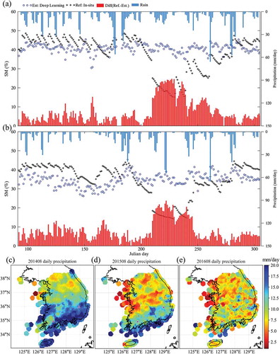
Figure 6. Variations in accuracy according to epochs (blue: training dataset, red: validation dataset).

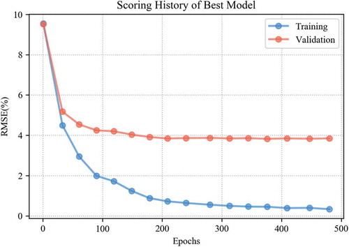
We set up a total of 25 models, as indicated in Table 4, which shows the summarized results of the grid search by accuracy in descending order. The results of the analysis indicated that a trained model with four hidden layers with 600 nodes each provided the most accurate result. Notably, the complexity of the neural network structure and the number of epochs were not directly proportional to accuracy. The simplest neural network had the lowest accuracy, while the most complicated neural network did not have the best accuracy. Likewise, there was not a linear relationship between the number of epochs for training and accuracy. According to the results, we selected four hidden layers of 600 nodes each as the best model to estimate SM. Figure 6 shows how to saturate the accuracy variation of the best model. Although there were some gaps in quantity, the variation trends in validation and training were quite similar. The errors tended to decrease sharply until the 90th learning time, and the error values tended to become somewhat flat after the 200th learning time.

Table 4. Summary of results by grid search.

Hidden Layer	R	R^2	RMSE	Epochs
[600, 600, 600, 600]	0.8918	0.7953	3.8246	480
[700, 700, 700, 700]	0.8895	0.7911	3.8633	582
[700, 700, 700]	0.8891	0.7904	3.8698	477
[600, 600, 600]	0.8887	0.7899	3.8750	429
[500, 500, 500, 500]	0.8884	0.7892	3.8809	435
[600, 600, 600, 600, 600]	0.8884	0.7892	3.8810	353
[300, 300, 300, 300, 300]	0.8855	0.7840	3.9284	491
[600, 600, 600, 600, 600, 600]	0.8854	0.7839	3.9294	564
[500, 500, 500]	0.8844	0.7822	3.9456	659
[400, 400, 400, 400]	0.8836	0.7807	3.9590	413
[500, 500, 500, 500, 500]	0.8832	0.7801	3.9639	372
[700, 700, 700, 700, 700, 700]	0.8831	0.7798	3.9669	317
[700, 700, 700, 700, 700]	0.8826	0.7790	3.9736	396
[400, 400, 400, 400, 400]	0.8825	0.7788	3.9760	379
[400, 400, 400]	0.8808	0.7759	4.0020	546
[300, 300, 300, 300]	0.8808	0.7758	4.0023	370
[700, 700, 700, 700, 700, 700, 700]	0.8772	0.7695	4.0581	333
[400, 400, 400, 400, 400, 400, 400]	0.8771	0.7693	4.0602	249
[400, 400, 400, 400, 400, 400]	0.8764	0.7680	4.0716	339
[500, 500, 500, 500, 500, 500]	0.8761	0.7675	4.0757	343
[600, 600, 600, 600, 600, 600, 600]	0.8760	0.7674	4.0773	414
[300, 300, 300, 300, 300, 300]	0.8736	0.7632	4.1134	329
[500, 500, 500, 500, 500, 500, 500]	0.8730	0.7621	4.1235	304
[300, 300, 300, 300, 300, 300, 300]	0.8717	0.7599	4.1418	295
[300, 300, 300]	0.8707	0.7581	4.1574	493

We conducted cross-validation (i.e. k-folds) to examine the stability of the selected neural network structure. Cook (2016) explained that 5 and 10 are common settings for n-folds; therefore, we set 10 as the n-number. Table 5 shows the detailed results of the k-folds process. All the results indicated high R values greater than 0.81 and low RMSE values less than 4.93. According to the results of cross-validation, the selected neural network structure had a low perturbation of 2% (R) and 4% (RMSE).

Table 5. The cross-validation metrics summary for estimated SM using a deep learning model.

	Mean	Std. Dev.	CV1	CV2	CV3	CV4	CV5	CV6	CV7	CV8	CV9	CV10
MAE	3.0467	0.1912	3.0124	2.8469	3.0446	3.0255	3.8062	2.9875	3.1152	2.8702	2.9734	2.7849
R	0.8630	0.0210	0.8714	0.8822	0.8626	0.8423	0.8106	0.8698	0.8568	0.8828	0.8700	0.8796
R^2	0.7448	0.0251	0.7593	0.7782	0.744	0.7095	0.6571	0.7565	0.7341	0.7793	0.7569	0.7737
RMSE	4.275	0.2086	4.1429	3.959	4.2341	4.6019	4.9309	4.1943	4.4901	3.9361	4.0766	4.183

4.4. Validation and comparison with other products

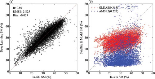
The SM calculated by the selected deep learning model was validated using a comparison to in-situ measurements. To assess the improvement by the deep learning model, we compared the accuracy of each SM dataset from AMSR2, GLDAS, and the deep learning model (Figure 7). The accuracy of the estimated SM using only the validation dataset shows a high R value (0.89) and low errors (RMSE: 3.825%, bias: −0.039%). The other SM products showed low R values (GLDAS: 0.365, AMSR2: 0.223) and relatively high RMSE (GLDAS: 9.030%, AMSR2: 20.622%) and bias (GLDAS: −4.201, AMSR2: −17.725). Furthermore, AMSR2 yielded a significantly lower SM, and GLDAS showed a relatively flat slope when compared with in-situ SM. In Figure 7, scatter plots of GLDAS and AMSR2 have different numbers of points (~ 3800 and 5100, respectively) because GLDAS regards the locations of the nine ground stations near the coast line as ocean surface due to its coarse spatial resolution of 0.25°.

Figure 7. Accuracy of the estimated SM using deep learning (a, black circle), GLDAS (b, red circle) and AMSR2 (b, blue cross) (each number beside the legend represents R).

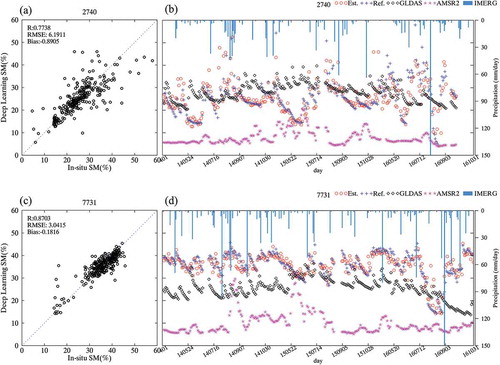
To examine the agreement in the time series, we compared the estimated SM in accordance with the two selected station locations (Figure 8) and in-situ measurements. Stations 2740 (R: 0.773, RMSE: 6.1911%, bias: −0.8905%) and 7731 (R: 0.8703, RMSE: 3.0415%, bias: −0.1816%) were selected as those with the lowest and highest accuracy, respectively. In Figure 8(b), the estimated SM shows a very similar variation trend and domain compared to those of the in-situ SM, except for several overestimations and underestimations after 16 July 2014, before 22 May 2015, and around 3 September 2016. Most of these errors were within a relatively high SM domain of over 35%, as shown in Figure 8(a). These errors may have been caused by concentrated heavy rain within a narrow spatial/temporal range not reflected in the satellite data because most of the errors occurred near rainfall. Furthermore, Station 2740 was in the middle of a mountainous area and had a large variation in DEM at a 4-km resolution (Std. Dev. of DEM: 61.29 m). Although there were several gaps in the estimated SM, it still had better performance than the SM of GLDAS (black diamond) and AMSR2 (violet star). In the case of Station 7731, the estimated SM had a significant agreement with the in-situ SM. AMSR2 had a steady low value and often an unusually high value by sensitively reflecting some rainfall (before 14 July 2015 in Figure 8(b) and after 22 May 2015 in Figure 8(d)). In the case of GLDAS, relatively similar variation trends were observed, but there was a constant gap with in-situ SM, as highlighted in Figure 8(d). Some sections around 24 May 2014 and 22 May 2015 had different variation trends and values regardless of the in-situ SM, as observed in Figure 8(b).

Figure 8. Scatter and time series plots to reveal variations between in-situ SM (blue cross) and other SM (deep learning: red circle, GLDAS: black diamond, AMSR2: violet star) with precipitation from IMERG (blue bar) for the highest (c and d: 7731) and lowest (a and b: 2740) accuracy stations.

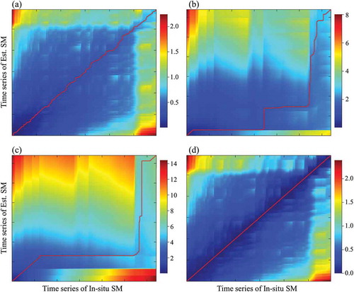
We tested the DTW of each SM time series to enhance intuitive analysis and comprehension of the similarities of each SM (Figures 9 and 10). DTW provided a more flexible comparison for similarities between the two time series than the traditional Euclidean method because it was calculated using Equations (1) and (2), as mentioned in Section 3.3. Figures 9(d) and 10(d) present the ideal result for DTW for in-situ measurements, establishing the reference result. As the two time series data became more similar, the D_ac had a more complete symmetry, and the warping path was closer to the diagonal position, as in Figures 9(d) and 10(d). Both warping paths of the SM from deep learning were nearly perfectly located at the diagonal position. Furthermore, the pattern and values of D_ac also showed strong similarities with both Figure 9(d) and 10(d). There was minimal fluctuation on the warping path, which was slightly different when other results were compared. The GLDAS warping path had more similarity with that of the in-situ SM than did AMSR2 at Station 2704. The warping paths of GLDAS (Figure 9(b)) and AMSR2 (Figure 9(c) and 10(c)) had trends leaning toward the x-axis because elements of D_ac were calculated by summing itself and its adjacent differences. The in-situ SM had a small range of fluctuations that occurred frequently, but there was little variation in the AMSR2, though large fluctuations occurred sometimes. Therefore, the warping path was shifted to one side during the process of finding similar fluctuations. In the variation of GLDAS, in-situ SM increased, but the GLDAS decreased after 24 May 2014 and the GLDAS repeatedly increased and decreased during one large fluctuation of in-situ SM before 20 May 2015 and 12 July 2016 (Figure 8(d)).

Figure 9. DTW results of each SM estimated using deep learning, GLDAS, and AMSR2 with in-situ SM for Station 2740 (a: deep learning, b: GLDAS, c: AMSR2, d: in-situ).

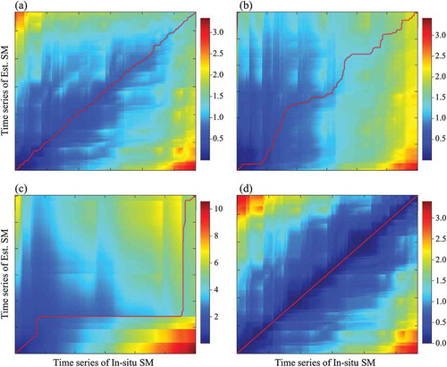
Figure 10. DTW results of each SM estimated using deep learning, GLDAS, and AMSR2 with in-situ SM in for Station 7731 (a: deep learning, b: GLDAS, c: AMSR2, d: in-situ).

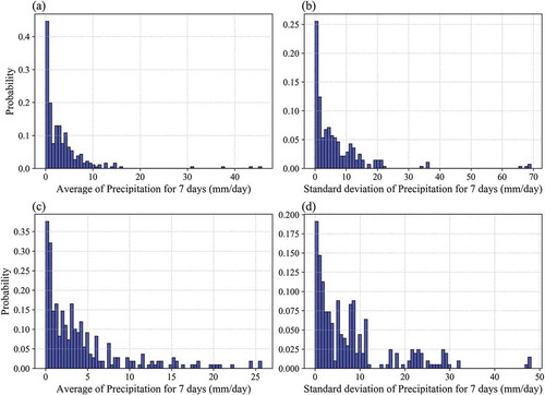
Finally, we analysed error trends in the estimated SM according to all input parameters except LC, because there were only four categories and their ranges were limited (Figure 11). Generally, the error patterns did not indicate bias from specific conditions and showed stable variations, except in precipitation. Most of the interquartile range (IQR) existed within ± 5%, and the mean values (asterisks) were located around the median line, indicating that the trained model reflected the variation of input parameters well. The errors of the estimated SM were uniformly distributed in a narrow area without being deflected to either plus or minus. In the precipitation graphs, the average precipitation for seven days increased, and the slight overestimation tendency was shown. However, for the last section in Figure 11(g) (~ 40–52 mm/day), the estimation was considerably underestimated. Due to the pattern of large amounts of precipitation in a small area, as mentioned in Section 4.1, IMERG precipitation with a relatively low resolution was considered to have underestimated the SM during rainfall above a certain level by inputting more rainfall than actually occurred (Figure 11(g)). Regarding the standard deviation of the precipitation (Figure 11(h)), the IQR of the error increased as the value of the interval increased, and it fluctuated in the positive and negative directions. The large standard deviation indicated that low and heavy rainfall coexisted for 7 days, and the mean increased and was overestimated. The results of analysis implied that our estimated SM accounted for the variation in input parameters, but the values for precipitation needed improvement regarding spatial resolution, because the precipitation values used in the model had relatively low spatial resolution and did not consider the recent pattern of precipitation with heavy rain in narrow areas. In Figure 12(c,d), Station 7731 shows relatively low average and standard deviation values of less than 25 and 50 mm/d, respectively. Station 2740, however, has high average and standard deviation values greater than 30 and 60 mm/day, respectively, in Figure 12(a,b). These differences lead to increasing errors, and these results are well matched to Figure 11 and the demonstrated effects of precipitation.

Figure 11. Boxplots of discrepancies in SM according to input variables (a: INS, b: OLR, c: NDVI, d: AL VIS, e: AL NIR, f: DEM, g: average of precipitation during seven days, i: standard deviation of precipitation during seven days).

Figure 12. The histogram of the average and standard deviation in IMERG precipitation during seven days (a: average of Station 2740, b: standard deviation of Station 2740, c: average of Station 7731, b: standard deviation of Station 7731).

5. Conclusion

We tested the training procedures of the deep learning model by reviewing sampling criteria, analysing the accuracy of the input variables, and assessing the stability of the model. Based on this analysis, we selected the model with the best performance. From the results of the cross-validation, our model has high R (0.86) and low RMSE (4.27) with a low fluctuation of 2% and 4%, respectively.

Our study indicated remarkably improved accuracy compared to the established SM values from satellites and models. Moreover, the bias was close to zero. The time series analysis revealed that the estimated SM showed the best performance with high agreement and similar values for the entire analysis period. In addition, we tested the similarity of three types of SM values to the in-situ SM using DTW. Results of the DTW analysis showed that the estimated SM was in near-perfect agreement with the in-situ SM.

The main advantage of our study is the improved reliability of drought monitoring. From a disaster prevention perspective, the estimated SM has relatively high spatial resolution compared to GLDAS (0.25°) and AMSR2 (0.1°), allowing for more detailed monitoring and improved notifications for residents. Moreover, since daily data production is possible, it can provide alerts and respond to droughts or a lack of SM faster than GLDAS (monthly) and AMSR2 (three-day delay). Although the data used to create a completely independent model covers only a short period, this can be overcome by the fusion of identical products from different satellites using cumulative distribution matching or optimal interpolation. This will be part of a future study. The suggested input parameters in this study can be easily adapted to other satellites and areas because it only uses level 2 products, and it reduces blank areas mainly using geostationary satellite data. The results of this study indicate that the spatial resolution can be improved using Himawari/AHI-8 or GK-2A/AMI data.

Acknowledgements

The authors acknowledge the National Institute of Agricultural Sciences, Rural Development Administration in Korea (http://rda.go.kr) for providing in-situ soil moisture data.

Disclosure statement

No potential conflict of interest was reported by the authors.

Additional information

Funding

This work was supported by the National Meteorological Satellite Center [Project No. 3137-305-210-13].

References

- Ahmad, S., A. Kalra, and H. Stephen. 2010. “Estimating Soil Moisture Using Remote Sensing Data: A Machine Learning Approach.” Advances in Water Resources 33: 69–80. doi:10.1016/j.advwatres.2009.10.008.
- Ali, I., F. Greifeneder, J. Stamenkovic, M. Neumann, and C. Notarnicola. 2015. “Review of Machine Learning Approaches for Biomass and Soil Moisture Retrievals from Remote Sensing Data.” Remote Sensing 7: 16398–16421. doi:10.3390/rs71215841.
- Bi, H., J. Ma, W. Zheng, and J. Zeng. 2016. “Comparison of Soil Moisture in GLDAS Model Simulations and in Situ Observations over the Tibetan Plateau.” Journal of Geophysical Research: Atmospheres 121 (6): 2658–2678. doi:10.1002/2015JD024131.
- Bolten, J. D., W. T. Crow, X. Zhan, T. J. Jackson, and C. A. Reynolds. 2010. “Evaluating the Utility of Remotely Sensed Soil Moisture Retrievals for Operational Agricultural Drought Monitoring.” IEEE Journal of Selected Topics in Applied Earth Observations and Remote Sensing 3 (1): 57–66. doi:10.1109/JSTARS.2009.2037163.
- Chang, D.-H., and S. Islam. 2000. “Estimation of Soil Physical Properties Using Remote Sensing and Artificial Neural Network.” Remote Sensing of Environment 74 (3): 534–544. doi:10.1016/S0034-4257(00)00144-9.
- Cho, E., H. Moon, and M. Choi. 2015. “First Assessment of the Advanced Microwave Scanning Radiometer 2 (AMSR2) Soil Moisture Contents in Northeast Asia.” Journal of Meteorological Society of Japan 93 (1): 117–129. doi:10.2151/jmsj.2015-008.
- Cho, J., Y.-W. Lee, P. J.-F. Yeh, K.-S. Han, and S. Kanae. 2014. “Satellite-Based Assessment of Large-Scale Land Cover Change in Asian Arid Regions in the Period of 2001-2009.” Environmental Earth Science 71 (9): 3935–3944. doi:10.1007/s12665-013-2778-0.
- Cook, D. 2016. Practical Machine Learning With H2O. Sebastopol, CA: O’Reilly.
- Crow, W. T., A. A. Berg, M. H. Cosh, A. Loew, B. P. Mohanty, R. Panciera, P. de Rosnay, D. Ryu, and J. P. Walker. 2012. “Upscaling Sparse Ground-Based Soil Moisture Observations for the Validation of Coarse-Resolution Satellite Soil Moisture Products.” Reviews of Geophysics 50: RG2002. doi:10.1029/2011RG000372.
- Didan, K., A. B. Munoz, R. Solano, and A. Huete, 2015. “MODIS Vegetation Index User’s Guide (MOD13 Series) Version 3.00.” Tucson, AZ: University of Arizona. https://vip.arizona.edu/documents/MODIS/MODIS_VI_UserGuide_June_2015_C6.pdf
- Elshorbagy, A., and K. Parasuraman. 2008. “On the Relevance of Using Artificial Neural Networks for Estimating Soil Moisture Content.” Journal of Hydrology 362 (1–2): 1–18. doi:10.1016/j.jhydrol.2008.08.012.
- Fang, L., C. R. Hain, X. Zhan, and M. C. Anderson. 2016. “An Inter-Comparison of Soil Moisture Data Products from Satellite Remote Sensing and a Land Surface Model.” International Journal of Applied Earth Observation and Geoinformation 48: 37–50. doi:10.1016/j.jag.2015.10.006.
- Fujii, H., T. Koike, and K. Imaoka. 2009. “Improvement of the AMSR-E Algorithm for Soil Moisture Estimation by Introducing a Fractional Vegetation Coverage Dataset Derived from MODIS Data.” Journal of Remote Sensing Society of Japan 29 (1): 282–292. doi:10.11440/rssj.29.282.
- Giraldo, M. A., M. Madden, and D. Bosch. 2013. “Land Use/Land Cover and Soil Type Covariation in a Heterogeneous Landscape for Soil Moisture Studies Using Point Data.” GIScience & Remote Sensing 46 (1): 77–100. doi:10.2747/1548-1603.46.1.77.
- Guan, X., C. Huang, G. Liu, X. Meng, and Q. Liu. 2016. “Mapping Rice Cropping Systems in Vietnam Using and NDVI-Based Time-Series Similarity Measurement Based on DTW Distance.” Remote Sensing 8 (1): 19. doi:10.3390/rs8010019.
- Huffman, G. J., D. T. Bolvin, D. Braithwaite, K. Hsu, R. Joyce, C. Kidd, E. J. Nelkin, S. Sorooshian, J. Tan, and P. Xie, 2017. “Algorithm Theoretical Basis Document (ATBD) Version 5.1 NASA Global Precipitation Measurement (GPM) Integrated Multi-satellitE Retrievals for GPM (IMERG), Global Precipitation Measurement (GPM) National Aeronautics and Space Administration (NASA).” https://pmm.nasa.gov/sites/default/files/document_files/IMERG_ATBD_V5.1_0.pdf
- Huffman, G. J., D. T. Bolvin, and E. J. Nelkin, 2017. “Integrated Multi-satellitE Retrievals for GPM (IMERG) Technical Documentation.” National Aeronautics and Space Administration Goddard Space Flight Center. http://pmm.nasa.gov/sites/default/files/document_files/IMERG_doc_171117b.pdf
- Im, J., S. Park, J. Rhee, J. Baik, and M. Choi. 2016. “Downscaling of AMSR-E Soil Moisture with MODIS Products Using Machine Learning Approaches.” Environmental Earth Sciences 75: 1120.
- Inoue, T., and S. A. Ackerman. 2002. “Radiative Effects of Various Cloud Types as Classified by the Split Window Technique over the Eastern Sub-Tropical Pacific Derived from Collocated ERBE and AVHRR Data.” Journal of Meteorological Society of Japan 80 (6): 1383–1394. doi:10.2151/jmsj.80.1383.
- JAXA Earth Observation Research Center. 2013. “Descriptions of GCOM-W1 AMSR2 Level 1R and Level 2 Algorithms.” https://suzaku.eorc.jaxa.jp/GCOM_W/data/doc/NDX-120015a.pdf
- Jeong, Y.-S., M. K. Jeong, and O. A. Omitaomu. 2011. “Weighted Dynamic Time Warping for Time Series Classification.” Pattern Recognition 44 (9): 2231–2240. doi:10.1016/j.patcog.2010.09.022.
- Jiang, Y., and Q. Weng. 2016. “Estimation of Hourly and Daily Evapotranspiration and Soil Moisture Using Downscaled LST over Various Urban Surfaces.” GIScience & Remote Sensing 54 (1): 95–117.
- Kawamura, H., S. Tanahashi, and T. Takahashi. 1998. “Estimation of Insolation over the Pacific Ocean off the Sanriku Coast.” Journal of Oceanography 54 (5): 457–464. doi:10.1007/BF02742448.
- Koike, T. 2013. “Soil Moisture Algorithm Descriptions of GCOM-W1 AMSR2 (Rev. A).” Earth Observation Research Center. Japan Aerospace Exploration Agency. http://suzaku.eorc.jaxa.jp/GCOM_W/data/doc/NDX-120015A.pdf
- Krizhevsky, A., I. Sutskever, and G. E. Hinton. 2012. “ImageNet Classification with Deep Convolutional Neural Networks.” In: Proceeding of Neural Information Processing Systems 25 (NIPS 2012), 1097-1105. Neveda, USA, December 3-8.
- Kaichi, M., K. Naoki, M. Hori, and K. Imaoka. 2013. “AMSR2 validation results.” In: Proceeding of IEEE International Geoscience Remote Sensing Symposium (IGARSS) 2013, 831-834. Melbourne, Canada, July 21-26.
- Lee, C. S., J. D. Park, J. Shin, and J.-D. Jang. 2017. “Improvement of AMSR2 Soil Moisture Products over South Korea.” IEEE Journal of Selected Topics in Applied Earth Observations and Remote Sensing 10 (9): 3839–3849. doi:10.1109/JSTARS.2017.273923.
- Li, X., G. Cheng, and L. Lu. 2005. “Spatial Analysis of Air Temperature in the Qinghai-Tibet Plateau.” Arctic, Antarctic, and Alpine Research 37: 246–252.
- Liang, S., X. Li, and J. Wang. 2012. Advanced Remote Sensing: Terrestrial Information Extraction and Application. 1st ed. Oxford, UK: Academic Press.
- Liou, Y.-A., S.-F. Liu, and W.-J. Wang. 2001. “Retrieving Soil Moisture from Simulated Brightness Temperatures by a Neural Network.” IEEE Transactions on Geoscience and Remote Sensing 39 (8): 1662–1672. doi:10.1109/36.942544.
- Ma, H., and S. Liu. 2016. “The Potential Evaluation of Multisource Remote Sensing Data for Extracting Soil Moisture Based on the Method of BP Neural Network.” Canadian Journal of Remote Sensing 42: 117–124.
- Mahdian, M. H., S. R. Bandarabady, R. Sokouti, and Y. N. Banis. 2009. “Appraisal of the Geostatistical Methods to Estimate Monthly and Annual Temperature.” Journal of Applied Sciences 9: 128–134.
- Mao, Y., Z. Wu, H. He, G. Lu, H. Xu, and Q. Lin. 2017. “Spatio-Temporal Analysis of Drought in a Typical Plain Region Based on the Soil Moisture Anomaly Percentage Index.” Science of the Total Environment 576: 752–765.
- Menzies, J., R. Jensen, E. Brondizio, E. Moran, and P. Mausel. 2013. “Accuracy of Neural Network and Regression Leaf Area Estimators for the Amazon Basin.” GIScience & Remote Sensing 44 (1): 82–92.
- Muller, M. 2007. Information Retrieval for Music and Motion. Heidelberg, Germany: Springer.
- Nair, V., and G. E. Hinton. 2010. “Rectified Linear Units Improve Restricted Boltzmann Machines.” In: Proceeding of the 27th International Conference on Machine Learning (ICML-10), 807–814. Haifa, Israel, June 21 –24.
- Nguyen, X. T., B. T. Nguyen, K. P. Do, Q. H. Bui, T. N. T. Hguyen, V. Q. Vuong, and T. H. Le. 2015. ““Spatial Interpolation of Meteorologic Variables in Vietnam Using the Kriging Method.” Journal of Information Processing System 11: 134–147.
- Oliva, R., E. Daganzo, Y. H. Kerr, S. Nieto, P. Richaume, and C. Gruhier. 2012. “SMOS Radio Frequency Interference Scenario: Status and Actions Taken to Improve the RFI Environment in the 1400-1427-Mhz Passive Band.” IEEE Transactions on Geoscience Remote Sensing 50 (5): 1427–1439. doi:10.1109/TGRS.2012.2182775.
- Padhee, S. K., B. R. Nikam, S. Dutta, and S. P. Aggarwal. 2017. “Using Satellite-Based Soil Moisture to Detect and Monitor Spatiotemporal Traces of Agricultural Drought over Bundelkhand Region of India.” GIScience & Remote Sensing 54 (2): 144–166.
- Park, J., and M. Choi. 2014. “Estimation of Evapotranspiration from Ground-Based Meteorological Data and Global Land Data Assimilation System (GLDAS).” Stochastic Environmental Research Risk Assessment 29 (8): 1963–1992. doi:10.1007/s00477-014-1004-2.
- Petitjean, F., J. Inglada, and P. Gancarski. 2012. “Satellite Image Time Series Analysis Under Time Warping.” IEEE Transactions on Geoscience and Remote Sensing 50 (8): 3081–3095. doi:10.1109/TGRS.2011.2179050.
- Petropoulos, G. P. 2013. Remote Sensing of Energy Fluxes and Soil Moisture Content. Florida, USA: CRC Press.
- Rodell, M., P. R. Houser, U. Jambor, J. Gottschalck, K. Mitchell, C.-J. Meng, K. Arsenault, et al. 2004. “The Global Land Data Assimilation System.” Bulletin of American Meteorological Society 85: 381–394. doi:10.1175/BAMS-85-3-381.
- Rodriguez-Fernandez, N. J., F. Aires, P. Richaume, Y. H. Kerr, C. Pregent, J. Kolassa, F. Cabot, C. Jimenez, A. Mahmoodi, and M. Drusch. 2015. “Soil Moisture Retrieval Using Neural Networks: Application to SMOS.” IEEE Transactions on Geoscience and Remote Sensing 53 (11): 5991–6007.
- Ryu, J.-H., K.-S. Han, and E.-B. Park. 2013. “Accuracy Evaluation of Near-Surface Air Temperature from ERA-interim Reanalysis and Satellite-Based Data according to Elevation.” Korea Society of Remote Sensing 29 (6): 595–600.
- Sakoe, H., and S. Chiba. 1978. “Dynamic Programming Algorithm Optimization for Spoken Word Recognition.” IEEE Transactions on Acoustics, Speech, and Signal Processing 26 (1): 43–49. doi:10.1109/TASSP.1978.1163055.
- Scientific, C., 1996. “Instruction Manual, CS615 Water Content Reflectometer, Version 8221-07.” Logan, UT: Campbell Scientific. http://s.campbellsci.com/documents/us/manuals/cs615.pdf
- Scientific, C., 2016. “Instruction Manual, CS616 and CS625 Water Content Reflectometers.” Logan, UT: Campbell Scientific. http://s.campbellsci.com/documents/us/manuals/cs616.pdf
- Seneviratne, S. I., T. Corti, E. L. Davin, M. Hirschi, E. B. Jaeger, I. Lehner, B. Orlowsky, and A. J. Teuling. 2010. “Investigating Soil Moisture-Climate Interactions in A Changing Climate: A Review.” Earth Science Reviews 99 (3–4): 125–161. doi:10.1016/j.earscirev.2010.02.004.
- Sharif, M., and A. A. Alesheikh. 2017. “Context-Awareness in Similarity Measures and Pattern Discoveries of Trajectories: A Context-Based Dynamic Time Warping Method.” GIScience & Remote Sensing 54 (3): 426–452. doi:10.1080/15481603.2017.1278644.
- Song, Y. M., W. D. Gua, and Y. C. Zhang. 2009. “Numerical Study of Impacts of Soil Moisture on the Diurnal and Seasonal Cycles of Sensible/Latent Heat Fluxes over Semi-Arid Region.” Advances in Atmospheric Sciences 26 (2): 319–326.
- Srivastava, P. K., D. Han, M. A. Ramirez, and T. Islam. 2013a. “Appraisal of SMOS Soil Moisture at a Catchment Scale in a Temperate Maritime Climate.” Journal of Hydrology 498: 292–304. doi:10.1016/j.jhydrol.2013.06.021.
- Srivastava, P. K., D. Han, M. R. Ramirez, and T. Islam. 2013b. “Machine Learning Techniques for Downscaling SMOS Satellite Soil Moisture Using MODIS Land Surface Temperature for Hydrological Application.” Water Resour Manage 27: 3127–3144.
- Strahler, A., D. Muchoney, J. Borak, M. Friedl, S. Gopal, E. Lambin, and A. Mody, 1999a. “MODIS Land Cover Product Algorithm Theoretical Basis Document (ATBD) Version 5.0 MODIS Land Cover and Land-Cover Change.” https://modis.gsfc.nasa.gov/data/atbd/atbd_mod12.pdf
- Strahler, A. H., J. P. Muller, W. Lucht, C. Schaaf, T. Tsang, F. Gao, X. Li, P. Lewis, and M. J. Barnsley. 1999b. “MODIS BRDF/albedo Product Algorithm Theoretical Basis Document Version 5.0.” MODIS Documentation 23 (4): 42–47. https://dratmos.geog.umd.edu/files/pdf/MODIS_BRDF.pdf.
- Yeom, J. M., C. S. Lee, S.-J. Park, -J.-J. Kim, H.-C. Kim, and K.-S. Han. 2015. “Evapotranspiration in Korea Estimated by Application of a Neural Network to Satellite Images.” Remote Sensing Letters 6 (6): 429–438. doi:10.1080/2150704X.2015.1041169.
- Yeom, J. M., and K.-S. Han. 2010. “Improved Estimation of Surface Solar Insolation Using a Neural Network and MTSAT-1R Data.” Computer & Geosciences 36 (5): 590–597. doi:10.1016/j.cageo.2009.08.012.
- Yeom, J. M., K.-S. Han, and Y. S. Kim. 2006. “Identification of Contaminated Pixels in 10-Day NDVI Image.” In: Proceedings of the Korean Society of Remote Sensing (KSRS) Spring C35Conference, 26-27. Dae-Jeon, South Korea, March 29-31.
- Zhang, D., W. Zhang, W. Huang, Z. Hong, and L. Meng. 2017. “Upscaling of Surface Soil Moisture Using a Deep Learning Model with VIIRS RDR.” ISPRS International Journal of Geo-Information 6 (5): 130.