Quality assessment of digital surface models extracted from WorldView-2 and WorldView-3 stereo pairs over different land covers

Abstract

Digital surface models (DSMs) extracted from very high resolution (VHR) satellite stereo images are becoming more and more important in a wide range of geoscience applications. The number of software packages available for generating DSMs has been increasing rapidly. The main goal of this work is to explore the capabilities of VHR satellite stereo pairs for DSMs generation over different land-cover objects such as agricultural plastic greenhouses, bare soil and urban areas by using two software packages: (i) OrthoEngine (PCI), based on a hierarchical subpixel mean normalized cross correlation matching method, and (ii) RPC Stereo Processor (RSP), with a modified hierarchical semi-global matching method. Two VHR satellite stereo pairs from WorldView-2 (WV2) and WorldView-3 (WV3) were used to extract the DSMs. A quality assessment on these DSMs on both vertical accuracy and completeness was carried out by considering the following factors: (i) type of sensor (i.e., WV2 or WV3), (ii) software package (i.e., PCI or RSP) and (iii) type of land-cover objects (plastic greenhouses, bare soil and urban areas). A highly accurate light detection and ranging (LiDAR) derived DSM was used as the ground truth for validation. By comparing both software packages, we concluded that regarding DSM completeness, RSP produced significantly (p < 0.05) better scores than PCI for all the sensors and type of land-cover objects. The percentage improvement in completeness by using RSP instead of PCI was approximately 2%, 18% and 26% for bare soil, greenhouses and urban areas respectively. Concerning the vertical accuracy in root mean square error (RMSE), the only factor clearly significant (p < 0.05) was the land cover. Overall, WV3 DSM showed slightly better (not significant) vertical accuracy values than WV2. Finally, both software packages achieved similar vertical accuracy for the different land-cover objects and tested sensors.

Keywords:

• DSM
• Worldview-2/3
• matching
• vertical accuracy
• completeness
• plastic greenhouse

1. Introduction

Digital Surface Models (DSMs) are one of the core products of very high resolution (VHR) satellite stereo photogrammetric imagery. Three-dimensional (3D) information plays a crucial role for many geospatial analysis (e.g. Maune 2007), adding accurate georeferenced datasets into Geographic Information Systems. With the development of spaceborne sensors, it is expected that VHR stereo data can be acquired in a timely and repeated manner for any region of interest, much more affordable than traditional aerial surveys. According to Noh and Howat (2015), the quality of stereoscopic DSMs depends on: (i) the radiometric and geometric quality of the imagery, (ii) the accuracy of the sensor model used to represent the relationship between image and object space, and (iii) the performance of the image matching algorithm.

Regarding radiometric and geometric quality of the imagery, the last investigations about extracting 3D information from VHR satellite stereo pairs are mainly focused on the new breed of DigitalGlobe’s VHR satellites such as GeoEye-1 and WorldView-1/2/3/4 (Aguilar, Saldaña, and Aguilar 2014; Noh and Howat 2015; Shean et al. 2016; Barbarella, Fiani, and Zollo 2017; DeWitt et al. 2017) which are capable of capturing panchromatic (PAN) imagery of the land surface with ground sample distance (GSD) even lower than 0.5 m. Others recently published works also pay attention to the capabilities of the PAN triplet from Pléiades-1 to generate DSMs (Poli et al. 2015; Di Rita, Nascetti, and Crespi 2017; Qin 2016).

The sensor model used at the stereo pair orientation phase can be particularly important for the DSM accuracy, and most of the state-of-the-art work take either the rigorous linear-array model or parametric rational polynomial function model (RPF) (Fraser, Baltsavias, and Gruen 2002; Toutin 2006; Capaldo et al. 2012; Crespi et al. 2012; Poli and Toutin 2012). As compared to rigorous model, the RPF model is concluded to be capable of achieving similar level of accuracy and being much more compatible across different sensors, thus nowadays is widely used as the standard geometric model for spaceborne optical images. The RPF builds the object-to-image space mapping through 78 parameters called RPC (rational polynomial coefficients). It should be noted that the initial RPC parameters derived from the satellite navigation system usually contain bias, thus the geo-referencing needs a bias-correction phase for generating precise epipolar images for dense image matching, which can be performed either using tie points (relative correction) or accurate ground control points (GCPs, for absolute correction) (Grodecki and Dial 2003; Fraser and Hanley 2003, 2005).

With regard to the image matching algorithm, there are many commercial software packages being able to procedure DSM from VHR stereo images such as MATCH-T, supplied by Trimble, LPS eATE, embedded into ERDAS, or Socet Set ATE, by BAE Systems. Among these, OrthoEngine, the photogrammetric module of Geomatica (PCI Geomatics), has been the most used in research works, serving as a benchmark for others packages in comparison tests (Capaldo et al. 2012; Fratarcangeli et al. 2016; Barbarella, Fiani, and Zollo 2017; Di Rita, Nascetti, and Crespi 2017). A few open source tools for DSMs generation from VHR satellite have become available such as Satellite Stereo Pipeline (S2P) (De Franchis et al. 2014), the NASA Ames Stereo Pipeline (ASP) (Shean et al. 2016), or Digital Automatic Terrain Extractor (DATE) (Di Rita, Nascetti, and Crespi 2017). In addition, RPC Stereo Processor (RSP) (Qin 2016) and the Surface Extraction with TIN-based Search-space Minimization (SETSM) (Noh and Howat 2017) represent other recently developed tools for DSM extraction. The aforementioned software packages use different image matching algorithms to find the corresponding image points. In that sense, Alobeid, Jacobsen, and Heipke (2010) concluded that the matching method for generating DSMs is crucial, especially in urban environments. They found that the area-based least squares matching is not able to generate sharp building outlines and strongly impacted by occlusions. On the other hand, semi-global matching (SGM) (Hirschmüller 2008) and dynamic programming matching method (Birchfield and Tomasi 1998) achieve better results working on urban areas.

It is important to note that DSM accuracy varies with the terrain surface roughness (Li 1992; Aguilar et al. 2005) and the target land-cover objects (Toutin 2006; Hobi and Ginzler 2012; Aguilar, Saldaña, and Aguilar 2014). A plethora of literature about DSMs generation from VHR satellite imagery over different study sites exists, including urban areas (Di Rita, Nascetti, and Crespi 2017), flat bare soil (Aguilar, Saldaña, and Aguilar 2014), mountainous areas (Fratarcangeli et al. 2016), densely vegetated deciduous forest (DeWitt et al. 2017), glaciated regions (Noh and Howat 2015) or over herb and grass land cover (Hobi and Ginzler 2012). However, to the best of our knowledge, few works have been specifically focused on greenhouse covered areas (Aguilar et al. 2014), where the different plastic materials with varying thickness, transparency, ultraviolet and infrared reflection and transmission properties, additives, age and colours are challenging for accurate 3D extraction. In recent years, plastic greenhouse mapping from remote sensing using spectral and texture features are receiving an increasing scientific interest (Aguilar et al. 2016; Novelli et al. 2016; Yang et al. 2017). As some of these works use VHR satellite imagery, the idea of adding 3D information (e.g., DSM or normalized digital surface model (nDSM)) to the classical spectral classification approach, can greatly improve the greenhouses mapping accuracy. In fact, it has already reported working with pixel-based and object-based supervised image classification algorithms (Aguilar et al. 2014; Celik and Koc-San 2018).

The vertical accuracy of a DSM generated from VHR satellite images is normally evaluated through highly accurate light detection and ranging (LiDAR) information as ground truth (Toutin 2006; Capaldo et al. 2012; Noh and Howat 2015). However, the generated DSM may not represent height for every single pixel due to matching errors provoked by insufficient texture, occlusions or radiometric artifacts. Therefore, DSM quality should also be evaluated using DSM completeness, defined as the percentage of correctly matched points over the area of interest (Höhle and Potuckova 2011).

The main objective of this paper is to evaluate and compare, exactly in the same conditions, the unfilled DSMs extracted from along-track WorldView-2 and WorldView-3 PAN VHR satellite stereo pairs over a very dense greenhouse covered area, also presenting mixed patches of bare soil and urban areas. Two software packages with two clearly different image matching approaches were also tested. In this sense, a DSM quality assessment, including both vertical accuracy and completeness, was performed to statistically analyse the effect of the following factors: (i) type of VHR sensor (i.e., WV2 or WV3), (ii) software package used (i.e., OrthoEngine or RSP) and (iii) type of land cover (plastic greenhouses, bare soil and urban areas).

2. Study sites

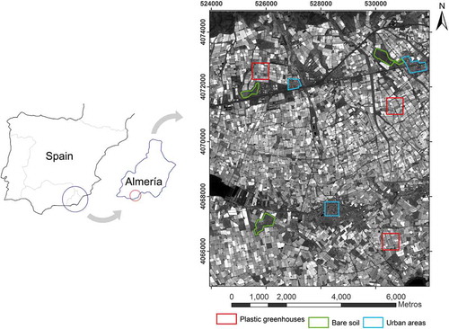
The study area is located in the province of Almeria (Southern Spain). It comprises an area of ca. 8000 ha centred on the geographic coordinates (WGS84) 36.7824°N and 2.6867°W (Figure 1). It is just at the core of the greatest concentration of greenhouses in the world, the so-called “Sea of Plastic” (Aguilar et al. 2015). This pilot area presents a smooth relief ranging between 152.6 and 214.8 m above mean sea level. Within the study area, nine sub-plots (red, green and blue polygons in Figure 1) with areas between 14 and 36 ha were selected according to their type of land cover. In fact, three sample areas of each land cover were selected so that they were representatives of plastic greenhouses, bare soil (practically without vegetation) and urban areas respectively.

Figure 1. Location of the study area in Almería (Spain). The nine selected subareas over plastic greenhouses, bare soil and urban areas are depicted as red, green and blue polygons respectively. Coordinate system: WGS84 UTM Zone 30N.

3. Datasets

3.1. WorldView-2 and WorldView-3 stereo pairs

A WorldView-2 (WV2) PAN along-track stereo pair was acquired on 5 July 2015 covering the study site (Table 1). It was collected in Stereo Ortho Ready Level-2A (StereoOR2A) format, presenting both radiometric and geometric corrections. StereoOR2A format is georeferenced to a cartographic projection using a surface of a constant height. It also counts on the corresponding RPC sensor camera model and metadata file. The delivered products were ordered with a dynamic range of 11 bits. The second stereo pair over the study site was collected on 11 July 2016. It was a PAN StereoOR2A product from WorldView-3 (WV3) with a dynamic range of 11 bits. The metadata including viewing geometry, sun positions and other acquisition parameters for both studied stereo pairs are shown in Table 1.

Table 1. Characteristics of panchromatic images from WorldView-2 (WV2) and WorldView-3 (WV3) stereo pairs.

Product	WV2 Stereo Pair		WV3 Stereo Pair
Images	WV2 Image 1	WV2 Image 2	WV3 Image 1	WV3 Image 2
Acquisition Date (D/M/Y)	5/7/2011	5/7/2011	11/07/2016	11/07/2016
Acquisition Time (GTM)	11:03	11:04	11:31	11:32
Scan direction	Forward	Forward	Forward	Forward
Off-Nadir View Angle	12.6º	24.6º	32.7º	22.2º
In-Track View Angle	8.3 º	−23.5 º	26.2 º	−2.8 º
Cross-Track View Angle	9.6 º	7.7 º	−20.3 º	−22.0 º
Satellite Azimuth	59.2º	172.7º	336.3º	273.6º
Collected GSD	0.484 m	0.550 m	0.422m	0.354 m
Product Pixel Size	0.5 m	0.5 m	0.3 m	0.3 m
Sun Azimuth	126.4º	126.9º	142.9º	143.5º
Sun Elevation	69.1º	69.3º	72.4º	72.5º

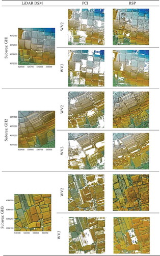
Figure 2. DSMs corresponding to the three subareas (samples) of greenhouse land cover (GH1, GH2 and GH3). First column: Original LiDAR (first and single returns). Second column: PCI derived DSMs from WV2 (1 m grid spacing) and WV3 (0.6 m grid spacing) stereo pairs. Third column: RSP derived DSMs from WV2 (1 m grid spacing) and WV3 (0.6 m grid spacing) stereo pairs.

3.2. Ground truth LiDAR data

The LiDAR data used as ground truth in this study was provided by the PNOA (National Plan of Aerial Orthophotograph of Spain) as a point cloud in LAS binary file, format v. 1.2 (Montealegre, Lamelas, and De La Riva 2015), containing easting and northing coordinates (UTM ETRS89 30N) and orthometric elevations (geoid EGM2008). It was captured on 23 September 2015, by a Leica ALS60 discrete return sensor with up to four returns measured per pulse and an average flight height of 2700 m. The registered point density of the test area, taking into account the overlapping, turned out to be 0.97 points/m² (all returns). The estimated vertical accuracy of the LiDAR data was computed on 131 GPS-RTK surveyed ground points evenly distributed over the whole study area. The standard deviation of the computed LiDAR vertical error, only including open terrain GCPs (Aguilar and Mills 2008), took a value of 0.14 m, meaning vertical accuracy higher than the 0.2 m nominal vertical error of PNOA LiDAR data (Montealegre, Lamelas, and De La Riva 2015).

The original density of the LiDAR point cloud was significantly reduced to extract a representative and yet manageable set of LiDAR points. In this sense, only single and first returns LiDAR points were used. Points from single return collect very well bare soil areas. However, the laser beam can capture several returns (on the top of the plastic cover, on the crop inside or on the bare soil) on plastic greenhouse. In that cases, in order to better represent the DSM ground truth from LiDAR data we selected the first return. After this, LiDAR data from the nine selected subareas were carefully edited by manually removing the points that did not belong to the DSM. This task was especially time consuming for the plastic greenhouse subareas where the first return LiDAR points sometimes and mainly depending on the plastic material, passed through the plastic sheet. It is important to note that if we want to obtain reliable results in the quality assessment of DSMs extracted from satellite stereo pairs, the LiDAR ground truth must represent in the best possible way the real DSM. Thus, the manually edition was extremely necessary, especially working with plastic greenhouses. Finally, a spatially oriented data thinning was carried out by sub-sampling the original point cloud using a minimum distance between points of 2 m. Following these steps, an evenly distributed ground truth LiDAR edited data over each study area of around 0.2 points/m² was obtained for validation.

4. Methodology

4.1. DSM Extraction from VHR Satellite Imagery

Two different software packages, based on different image matching approaches, were used to stereo-photogrammetrically generate the DSM from WV2 and WV3 stereo pairs.

OrthoEngine, the photogrammetric module of Geomatica v. 2013 software (PCI Geomatics, Richmond Hill, ON, Canada) was the first of the packages tested. OrthoEngine (PCI henceforth) matching algorithm is based on cross-correlation where an automated area-based matching procedure is performed on quasi-epipolar images. Specifically, this procedure utilizes a hierarchical sub-pixel mean normalized cross correlation matching method that generates correlation coefficients between zero and one for each matched pixel, where zero represents a total mismatch and one a perfect match. When the correlation coefficient of a matched point is lower than 0.5, this point is rejected and its height is not computed, meaning a gap and reducing the DSM completeness. Finally, a second-order surface is then fitted around the maximum correlation coefficients to find the match position to sub-pixel accuracy (Chen 2015).

RSP (RPC Stereo Processor) was the other software package tested in this work. RSP was initially developed by Qin (2014) for 3D change detection and land cover classification studies and it was further refined as a standalone software package that performs stereo matching on RPC modelled space-borne images producing mapping products such as DSM and orthophoto (Qin 2016). RSP implements a hierarchical SGM approach based on the widely known algorithm proposed by Hirschmüller (2008) to generate the disparity maps after applying an epipolar rectification process to the original stereo images.

The sensor orientation phase for both software packages was carried out by the empirical model based on a third-order 3-D rational functions with vendor’s RPCs data and refined by a zero-order polynomial adjustment (RPC0), following the block adjustment method published by Grodecki and Dial (2003) for image space. Although RPC0 requires only one GCP, and in order to have a better reliability, seven GPS-RTK surveyed ground points evenly distributed over the working area were used following the recommendations of Aguilar, Saldaña, and Aguilar (2013). It is important to keep in mind that the GCPs were only marked once on the image space of the PCI project, being later exported to be automatically marked in the RSP project in order to guarantee the same input. Exactly the same seven GCPs were used to perform the sensor orientation for WV2 and WV3.

After carrying out the sensor orientation phase, four grid spacing format DSMs for each subarea were stereo-photogrammetrically extracted by using different combinations of sensor (WV2 and WV3) and software packages (PCI and RSP). The DSMs were always computed in orthometric elevations using the EGM2008 geoid. The resolution of these DSMs was set to 0.6 m and 1 m for WV3 and WV2 respectively (two times of the image GSD). In the case of PCI, “hilly terrain” and “without filling blanks” (no interpolation) parameters were chosen. In the case of the RSP software, the DSM was also extracted without filling blanks. Finally, 36 unfilled DSMs were extracted (9 subareas × 2 software packages × 2 sensors).

4.2. Quality assessment of the extracted DSMs

The quality of the extracted DSMs was assessed by computing their completeness and vertical accuracy. As mentioned, the quality assessment was focused on different software packages, sensors and land covers. Thus, three samples of three types of land cover (plastic greenhouses, bare soil and urban areas) were considered within the study area, finally leading to the nine test subareas as shown in Figure 1.

The completeness of every DSM was computed for the different studied subareas as the ratio between the number of correctly matched points and the maximum possible number of points for the selected DSM grid spacing. Therefore, the completeness offers a quantitative measure about the influence of the different tested factors on the ability to extract local 3D information over the study area.

Regarding the accuracy of the stereo-photogrammetrically extracted DSMs from the WV2 and WV3 stereo pairs in the nine subareas, the 3D points from the manually edited LiDAR DSM were employed as independent check points (ICPs) for assessing the vertical accuracy (LiDAR ICPs), computing vertical residual (z-residual) at each corresponding point as photogrammetric height minus LiDAR height. It is important to note that each ICP will produce a z-residual if the area around the planimetric position of this ICP contains height information in the corresponding DSM. In this case, a bilinear interpolation was used to compute the value of that z-residual. For instance, in the case of the first repetition of plastic greenhouses land cover (area of 36 ha), 58,909 LiDAR ICPs were considered as ground truth. However, the total number of successfully extracted z-residuals was fewer in photogrammetrically derived DSMs due to matching algorithm failures (i.e., the completeness values of the DSMs for each subarea were always lower than 100%). In fact, for this subarea different numbers of total extracted z-residuals (Total z-residuals) were computed from PCI WV2 DSM (38,049), RSP WV2 DSM (52,084), PCI WV3 DSM (36,654) and RSP WV3 DSM (49,119). To fully complete the picture, the vertical accuracy assessment for each subarea was also performed only on those ICPs where z-residuals were available for all the sensors and software packages tested in each subarea (i.e., Common ICPs), thus reducing the number of ICPs but ensuring a fair play in the comparison on different factors. In our example corresponding to the first repetition of greenhouse land cover, the final number of ICPs at which z-residuals could be computed in all cases stood at 26,109 for PCI WV2 DSM, RSP WV2 DSM, PCI WV3 DSM and RSP WV3 DSM. In that sense, two strategies have been carried out in this work for assessing vertical accuracy from VHR satellite derived DSMs: (i) using all the ICPs from each subarea and combination of software/sensor, and (ii), for ensuring a fair comparison, using only those ICPs where the z-residuals were available for all the sensors and software tested in each subarea. After removing blunders from the z-residuals populations attained from both strategies by applying the widely known three-sigma rule (Daniel and Tennant 2001), statistics such as Mean, Standard Deviation (SD), vertical Root Mean Squared Error (RMSE) and 95th (LE95) percentile Linear Error were computed for the final vertical accuracy assessment. These statistics are usually adopted for the assessment of DSMs (Di Rita, Nascetti, and Crespi 2017).

The number of ICPs from the manually edited LiDAR point cloud, the total number of ICPs which produced z-residuals in each subarea and the number of z-residual attained on common ICPs are depicted in Table 2 for all the studied factors. It is worth noting that the figures depicted in Table 2 are the mean values of three samples.

Table 2. Number of ICPs from the manually edited LiDAR point cloud (LiDAR ICPs), number of all ICPs with z-residuals (Total z-residuals) and number of common LiDAR ICPs which produce z-residuals from the photogrammetrically derived DSMs (Common ICPs), for all the studied cases (i.e., land cover, sensor and software). The depicted figures are given as mean values of three samples or repetitions while the range (Minimum, Maximum) are presented in brackets and italic font.

		WV2			WV3
Type of land cover	No. ICPs and z-residuals	PCI	RSP		PCI	RSP
	LiDAR ICPs	55,609.7 (51,920, 58,909)	55,609.7 (51,920, 58,909)		55,609.7 (51,920, 58,909)	55,609.7 (51,920, 58,909)
Greenhouse	Total z-residuals	41,824.7 (38,049, 45,797)	53,018.3 (51,432, 55,539)		36,997 (33,557, 40,780)	49,304 (47,409, 51,384)
	Common ICPs	29,457.7 (26,109, 33,816)	29,457.7 (26,109, 33,816)		29,457.7 (26,109, 33,816)	29,457.7 (26,109, 33,816)
	LiDAR ICPs	41,050 (25,794, 50,679)	41,050 (25,794, 50,679)		41,050 (25,794, 50,679)	41,050 (25,794, 50,679)
Urban	Total z-residuals	22,346.3 (14,781, 26,167)	39,090.7 (24,798, 47,547)		24,514.7 (15,269, 29,955)	35,951.7 (22,876, 42,892)
	Common ICPs	14,419 (9246, 18,103)	14,419 (9246, 18,103)		14,419 (9246, 18,103)	14,419 (9246, 18,103)
	LiDAR ICPs	36,163.3 (20,588, 45,087)	36,163.3 (20,588, 45,087)		36,163.3 (20,588, 45,087)	36,163.3 (20,588, 45,087)
Bare Soil	Total z-residuals	34,654 (19,886, 43,032)	36,113.7 (20,560, 45,078)		35,621 (20,195, 44,495)	36,009.3 (20,445, 44,968)
	Common ICPs	34,082.7 (19,622, 42,658)	34,082.7 (19,622, 42,658)		34,082.7 (19,622, 42,658)	34,082.7 (19,622, 42,658)

In order to study the statistical influence on DSM quality attributed to the three factors studied in this work, an experimental design based on a factorial model with three samples was implemented. Since the residual populations (z-residuals at ICPs) did not always fit a normal distribution, the Kruskal-Wallis H test (Spurrier 2003), a well-known rank-based non-parametric test, was applied to determine if there were statistically significant differences (p < 0.05) between two or more groups of an independent variable or factor (land cover, software package or sensor) in relation to a quantitative dependent variable (DSM quality statistics such as Mean, SD, RMSE, LE95 and Completeness).

5. Results and discussion

5.1. Visual inspection

Figures 2, 3 and 4 show the three-dimensional shaded relief for the different satellite derived DSMs produced in this work. Overall, these figures visually show that RSP software package achieved better results (in terms of completeness) than PCI for both WV2 and WV3 satellites, especially on urban areas and plastic greenhouses. A more detailed analysis of each figure is presented in below.

Figure 3. DSMs corresponding to the three subareas (samples) of urban areas (UR1, UR2 and UR3). First column: Original LiDAR (first and single returns). Second column: PCI derived DSMs from WV2 (1 m grid spacing) and WV3 (0.6 m grid spacing) stereo pairs. Third column: RSP derived from WV2 (1 m grid spacing) and WV3 (0.6 m grid spacing) stereo pairs.

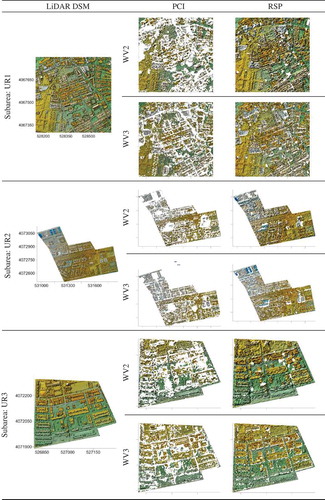
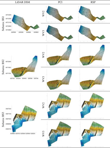
Figure 4. DSMs corresponding to the three subareas (samples) of bare soil land cover (BS1, BS2 and BS3). First column: Original LiDAR (first and single returns). Second column: PCI derived DSMs from WV2 (1 m grid spacing) and WV3 (0.6 m grid spacing) stereo pairs. Third column: RSP derived DSMs from WV2 (1 m grid spacing) and WV3 (0.6 m grid spacing) stereo pairs.

In Figure 2, the first column shows the original LiDAR data for the three samples of greenhouse land cover (subareas GH1, GH2 and GH3) with a grid spacing of 0.6 m. It is noteworthy that the little water irrigation ponds located at these agricultural areas did not have any first or single LiDAR return. Leica ALS60, as most of the LiDAR systems today, is set up to work over land using an infrared beam which tends to be absorbed by water, so over water bodies there are what are called data voids. These three LiDAR DSMs in Figure 2 can be visually compared to the DSMs derived from the WV2 and WV3 stereo pairs by using both PCI and RSP software packages. Through this visual inspection, the SGM implemented in RSP software achieved much better results than PCI algorithm for both WV2 and WV3 satellites in terms of the completeness. It is important to note that the WV2 DSMs over greenhouses seem to show a smaller number of missing image matching points than WV3 DSMs, although this fact should be statistically confirmed in the next section.

The DSMs of the three samples over urban areas (UR1, UR2 and UR3) are shown in Figure 3. Again, the completeness achieved by using RSP yielded much better results than PCI software for both WV2 and WV3 imagery.

Concerning the bare soil land cover (Figure 4), the quality of the DSMs derived from WV2 and WV3 stereo pairs appear similar to the quality of the LiDAR derived DSM in the three subareas (BS1, BS2 and BS3). The completeness was close to 100% for all the studied cases in Figure 4, although again RSP presented a slightly better rate of matching points than PCI.

5.2. DSM completeness

In this section we analysed the DSM completeness from a statistical point of view. Table 3 shows the completeness scores computed for all the 12 studied cases (i.e., three land covers, two sensors and two software packages). It should be noted that three samples for each case were considered (i.e., 36 VHR satellite derived DSMs). In order to summarize the results, the mean, maximum and minimum values of completeness are shown in Table 3. From the global statistical analysis of the completeness values using Kruskal-Wallis H test, it can be concluded that both land cover and software package factors turned out to be significant (p < 0.05).

Table 3. Mean and range of values (maximum and minimum) of completeness attained from the three samples per land cover. Different superscript letters between data along Completeness column indicate significant differences at a significance level p < 0.05.

Land Cover		Sensor	Software	Completeness (%)	Max. (%) – Min. (%)
Greenhouse		WV2	PCI	82.53^b	86.00 – 76.42
			RSP	97.92^de	99.06 – 95.66
		WV3	PCI	70.83^a	75.42 – 67.42
			RSP	91.49^cd	92.18 – 90.40
Urban	WV2		PCI	65.55^a	67.49 – 63.97
			RSP	94.83^cde	95.57 – 93.40
	WV3		PCI	66.39^a	69.21 – 63.67
			RSP	89.59^c	90.80 – 87.19
Bare Soil		WV2	PCI	97.83^de	98.85 – 96.75
			RSP	99.94^e	100.00 – 99.82
		WV3	PCI	99.27^e	99.40 – 99.17
			RSP	99.97^e	99.99 – 99.94

The land cover was the main contributing factor, presenting a partial eta-squared statistic (η_p²) of 64.18%, meaning that 64.18% of the completeness variance is statistically explained by the land cover factor. The best completeness score (p < 0.05) was achieved for bare soil with a mean value for the 12 cases shown in Figure 4 of 99.25%. The other two land covers did not present statistical significant differences (p < 0.05) with respect to mean values of completeness for the 12 DSMs shown in Figures 2 and 3 (mean completeness value of 85.69% for Greenhouse land cover and 79.09% for Urban land cover). Aguilar, Saldaña, and Aguilar (2014), in their previous study by using PCI software, reported DSM completeness values over urban areas of 63.23% and 78.83% working from GeoEye-1 and WV2 stereo pairs respectively. In the current study DSM completeness values by applying PCI provided scores of 65.55% and 66.39% from WV2 and WV3 stereo pairs respectively (Table 3).

Turning to the global statistical analysis, the portion of variance explained by the software package turned out to be much lower (η_p² = 26.36%). In this regards, the DSMs generated by RSP yielded a completeness mean value of 95.62%, whereas the DSMs produced through PCI software achieved a mean value of 80.40%. Overall, the improvement completeness by using RSP software package instead of PCI was about 2%, 18% and 26% for bare soil, greenhouses and urban areas respectively.

When per-class statistical analysis of completeness focusing on each land cover was performed, the software package factor proved to be significant (p < 0.05), with similar η_p² values of around 75.60% for each land cover studied. However, the difference in mean completeness values due to the software was very small for bare soil, while comparatively it was much more important in urban and greenhouse areas. In Table 3, mean values of completeness in the same column followed by different superscript letters are indicating significant differences at p < 0.05. Therefore, the four completeness scores attained on bare soil land cover for each combination of sensor and software were not significant since all the values were followed of the same “e” letter. In the case of greenhouse and urban land cover, RSP completeness values turned out to be significant better than PCI for the same land cover and sensor (Table 3). According to Alobeid, Jacobsen, and Heipke (2010), area-based matching algorithms (e.g., PCI software) usually present problems to generate clear building outlines on urban areas, while the SGM algorithm (e.g., RSP) achieves better results on the roof structures and boundaries.

Regarding sensor factor, the η_p²values were of 2.11%, 3.72% and 18.88% for bare soil, urban and greenhouse respectively. It is important to note that completeness values were only affected by the type of sensor in the case of greenhouse land cover, although statistical analysis revealed that this effect was quite moderate (p < 0.15). The completeness was always worse for WV3 (Table 3) in the case of the greenhouse land cover. It was mainly attributed to the stereo pairs viewing geometry and its relationship with the sun position. In certain situations, the plastic cover of the greenhouses may induce specular reflection of sun light, thus causing unusually bright pixel digital values (sun glint effect). This effect contributes to increase the number of missing image matching points. In that sense, the viewing geometry of the WV3 stereo pair produced much more greenhouses affected by glint than WV2. In fact, the two images composing the WV3 stereo pair were collected just in front of the sun position (see satellite and sun azimuth in Table 1), while the WV2 images left the sun on their back (Table 1).

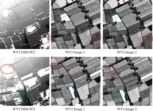
The relationship between DSM completeness and the glint effect over greenhouse plastic cover is shown in Figure 5. In this figure, the WV2 and WV3 DSMs produced by using PCI software package are depicted alongside the original PAN images from both stereo pairs for the GH2 subarea. The red ellipses highlight greenhouses presenting visible radiometric anomalies due to glint effect in one of the stereo pair images, thus causing matching errors. However, and when the greenhouses also present extreme values of digital number because they are painted white (plastic sheets may be painted white during summer to protect plants from excessive radiation and to reduce the heat inside the greenhouse), the matching algorithm works well. These painted greenhouses are marked in blue ellipses in Figure 5 and there are no radiometric changes in the stereo pair images. It is important to bear in mind the geometric configuration between the sun and sensor positions when the satellite image is acquired. Wulder et al. (2008) reported important changes in shadow size and orientation due to the interaction of sun position and VHR satellite geometry, resulting in inconsistent classification over different scenes.

Figure 5. Influence of glint effect over greenhouse plastic cover in relation to DSM completeness at GH2 subarea (600 m x 600 m). WV2 DSM produced by PCI and the original PAN images from WV2 stereo pair are shown in the first row. WV3 DSM produced by PCI and the original PAN images from WV3 stereo pair are shown in the second row. Blue ellipses mark greenhouses painted white and red ellipses highlight greenhouses presenting glint changes.

5.3. DSM vertical accuracy

DSM vertical accuracy assessment results (Mean, SD, RMSE and LE95) corresponding to each land cover, sensor and software packages when all the points from the manually edited LiDAR DSMs were employed as ICPs and all z-residuals considered (Total z-residuals) are depicted in Table 4. The land cover was the only statistically significant factor (p < 0.05) when random errors were assessed following a global statistical analysis through the Kruskal-Wallis test including all the 36 cases. Very similar and high values of η_p² were obtained for RMSE (87.34%), SD (88.34%) and LE95 (88.34%). For instance, significant (p < 0.05) mean SD values (12 cases) of 0.89 m, 2.17 m and 0.23 m were achieved for greenhouse, urban and bare soil areas respectively. As for global statistical analysis related to systematic errors, measured as mean or bias values, the land cover (η_p² = 18.86%) and sensor (η_p² = 12.83%) turned out to be significant (p < 0.05) factors, although this parameter presented a very high uncertainty. It is worth noting that the software package did not show any influence in the global accuracy assessment for both random and systematic errors despite that RSP presented far better completeness values than PCI.

Table 4. Vertical accuracy (Mean, SD, RMSE and LE95) computed on the all ICPs. All the depicted values are mean values corresponding to three samples for each land cover. Minimum and Maximum values for the three samples are depicted in brackets and italic font for Mean and SD. Different superscript letters between data along the same column indicate significant differences at a significance level p < 0.05.

Land Cover	Sensor	Software	Mean (m)	SD (m)	RMSE (m)	LE95 (m)
Greenhouse	WV2	PCI	−0.08 (−0.31, 0.11)	0.81^ab (0.70, 0.94)	0.83^ab	2.03^a
		RSP	−0.11 (−0.47, 0.34)	1.10^abc (0.93, 1.30)	1.16^abc	2.83^abc
	WV3	PCI	−0.21 (−0.41, −0.02)	0.82^ab (0.71, 1.03)	0.86^ab	2.12^a
		RSP	−0.47 (−0.92, 0.34)	0.84^ab (0.80, 0.87)	1.16^abc	2.54^ab
Urban	WV2	PCI	0.10 (−0.04, 0.22)	2.12^cd (1.74, 2.73)	2.12^cd	5.21^cd
		RSP	−0.27 (−0.61, −0.07)	2.92^d (2.32, 3.66)	2.95^d	7.23^d
	WV3	PCI	−0.41 (−0.54, −0.32)	1.89^bcd (1.43, 2.72)	1.94^bcd	4.83^bc
		RSP	−0.54 (−0.77, −0.27)	1.75^bc (1.31, 2.73)	1.85^bc	4.62^bc
Bare Soil	WV2	PCI	0.23 (0.19, 0.32)	0.25^a (0.22, 0.29)	0.34^a	0.67^a
		RSP	−0.03 (−0.08, −0.01)	0.28^a (0.23, 0.31)	0.28^a	0.56^a
	WV3	PCI	0.07 (−0.20, 0.32)	0.21^a (0.17, 0.25)	0.30^a	0.57^a
		RSP	−0.08 (−0.32, 0.10)	0.20^a (0.14, 0.23)	0.26^a	0.48^a

Focusing on the 12 DSMs corresponding to the bare soil land cover in Figure 4, only the sensor factor for SD was pointed out significant (p < 0.05) with a η_p² value of 39.39%. In the case of bare soil land cover, the DSMs generated by WV3 presented significantly better accuracy in terms of SD (0.20 m) than in the case of WV2 (SD = 0.26 m). However, this improvement could not be confirmed when working with RMSE or LE95. Worse SD values of 0.40 m and 0.53 m were attained by Aguilar, Saldaña, and Aguilar (2014) over bare soil areas from GeoEye-1 and WV2 stereo pairs respectively. Shean et al. (2016) and Noh and Howat (2015) achieved around approximately 0.21 m vertical RMSE with WorldWiew-1 and WV2 stereo pairs in glaciated regions, and in both cases removing the offsets through co-registration. A small error in planimetric coordinates between LiDAR data and the photogrammetrically derived DSM (incorrect co-registration) can lead to a systematic shift in height (Z coordinate). This can easily be spotted by visual analysis of the value of the residual over the area to check for spatial patterns which reproduce geomorphology of terrain or features (see for example the Figure 3f published by Aguilar, Saldaña, and Aguilar (2014)). It is worth mentioning that a finer co-registration process could have been carried out in our work.

Regarding the partial accuracy assessment statistical analysis over the unique greenhouse land cover (12 DSMs in Figure 2), significant differences (p < 0.05) were only achieved for the software package factor in the cases of RMSE and LE95. In both measures, PCI yielded better accuracy values (RMSE = 0.85 m and LE95 = 2.07 m) than RSP (RMSE = 1.16 m and LE95 = 2.69 m). It is important to bear in mind that RSP presented higher completeness in DSM generation than PCI, especially for greenhouse and urban areas. Thus, the worse vertical accuracy results attained over greenhouses in the case of RSP seem to point to the fact that RSP is incurring a commission error when working on difficult-to-match image areas (i.e., some greenhouse roofs presenting glint effect or very transparent plastic cover). This hypothesis is supported by the fact that both software packages did not show any accuracy differences over bare soil land cover with similar completeness and without glint or transparency problems.

In the case of urban subareas depicted in Figure 3, none of the vertical accuracy statistics led to significant (p < 0.05) for both sensor and software factors. As in the previous case, PCI presented better accuracy values than RSP for the WV2 stereo pair. However, in the case of WV3, RSP had a slightly better performance in terms of SD, RMSE and LE95. RMSE and SD values resulted to be significantly better at 0.10 signification level for WV3 (RMSE = 1.90 m and SD = 1.82 m) than in the case of WV2 (RMSE = 2.53 m and SD = 2.52 m). In view of these figures, it seems that the better GSD of the WV3 DSMs yielded better vertical accuracy results in very uneven urban land cover. Using a similar methodology on GeoEye-1 and WV2 stereo pairs Aguilar, Saldaña, and Aguilar (2014) achieved SD values over urban areas located in Southern Spain of 2.67 m and 2.74 m. On the other hand, Poli et al. (2015) reported higher vertical RMSE values on urban areas ranging from 6.1 m to 8.5 m by using GeoEye-1, WV2 and Pléiades-1A stereo images, although they tested the accuracy of filled DSMs (i.e., areas without successful matching 3D points were interpolated). Di Rita, Nascetti, and Crespi (2017) compared two software packages in urban areas (DATE, based on SGM and PCI) to produce DSMs from Pléiades-HR and GeoEye-1 stereo pairs. Although they worked with the filled DSMs, the obtained accuracy statistics were quite similar, with slight better performances of DATE with Pléiades and of PCI with GeoEye-1.

Finally, if a statistical analysis is performed for the values depicted in the columns of Table 4, we can conclude that there was no difference (i.e., no superscript) between systematic errors or Mean values. Regarding random errors, the best accuracy attained for bare soil land cover, WV3 and RSP (e.g., SD = 0.20 m) was not significantly different of the rest of accuracy values computed for bare soil and greenhouse land cover because all these figures are followed of the letter “a” (Table 4). The random errors for urban land cover without letter “a” in Table 4 were significantly worse than for bare soil.

So far, the statistical analysis on vertical accuracy of VHR satellite DSMs, especially on greenhouse and urban land covers, varied with their differences in completeness. In order to avoid this dependence and ensure a fair comparison, a second strategy was conducted. Table 5 shows the results for the DSM vertical accuracy assessment (Mean, SD, RMSE and LE95) by using only the Common ICPs (see Table 2) producing z-residuals in each subarea. Values in each column followed of different superscript letters presented significant differences (p < 0.05). The application of this strategy provided much clearer and more conclusive results. In fact, the systematic errors were not significant (p < 0.05) for any factor, and the random errors turned out to be significant at 0.05 level only for the land-cover factor. In that way, the best global SD mean values computed on 12 cases were obtained for bare soil (SD = 0.22 m), followed by greenhouse (SD = 0.71 m), and finally, urban areas (SD = 1.53 m).

Table 5. Vertical accuracy assessment (Mean, SD, RMSE and LE95) restricted to only common ICPs with z-residuals in each subarea. All the depicted values are mean values corresponding to three samples for each land cover. Minimum and Maximum values for the three samples are depicted in brackets and italic font for Mean and SD. Different superscript letters between data along the same column indicate significant differences at a significance level p < 0.05.

Land Cover		Sensor	Software	Mean (m)	SD (m)	RMSE (m)	LE95 (m)
Greenhouse		WV2	PCI	−0.09 (−0.30, 0.09)	0.76^ab (0.67, 0.87)	0.78^ab	1.87^ab
			RSP	−0.22 (−0.48, 0.13)	0.76^ab (0.66, 0.82)	0.83^abc	1.85^ab
		WV3	PCI	−0.20 (−0.40,-0.00)	0.72^ab (0.64, 0.88)	0.77^ab	1.87^ab
			RSP	−0.50 (−0.92, 0.20)	0.58^ab (0.50, 0.67)	0.91^abc	1.77^ab
Urban	WV2		PCI	0.07 (−0.09, 0.16)	1.68^c (1.37, 2.27)	1.69^c	4.24^c
			RSP	−0.02 (−0.09, 0.16)	1.67^c (1.32, 2.35)	1.68^c	4.30^c
	WV3		PCI	−0.16 (−0.38, 0.10)	1.46^bc (1.06, 2.11)	1.49^bc	3.84^bc
			RSP	−0.33 (−0.67, −0.13)	1.31^bc (0.92, 1.96)	1.39^bc	3.54^bc
Bare Soil		WV2	PCI	0.23 (0.18, 0.32)	0.24^a (0.22, 0.28)	0.34^a	0.66^a
			RSP	−0.03 (−0.07, −0.01)	0.26^a (0.21, 0.30)	0.26^a	0.53^a
		WV3	PCI	0.07 (−0.20, 0.31)	0.20^a (0.16, 0.24)	0.29^a	0.56^a
			RSP	−0.08 (−0.32, 0.10)	0.19^a (0.13, 0.23)	0.25^a	0.47^a

The results for the bare soil land cover were very similar to those aforementioned in Table 4. It is needed to bear in mind that the completeness values in this land cover were always very close to 100%. Again the DSMs generated by WV3 yielded significantly (p < 0.05) better accuracy only in terms of SD. Both software packages worked very well and without significant differences in vertical accuracies for this land cover.

For greenhouse land cover, neither the sensor nor the software factors were significant at 0.05 signification level for Mean, SD, RMSE or LE95. When the residuals were only computed in those LiDAR ICPs successfully matched by the two tested software (Common ICPs), overall, the vertical accuracy measures yielded better values. This fact was particularly important for RSP software package where, for instance, the SD value was improved around of 0.30 m. In the case of Common ICPs strategy, the vertical accuracy results for the two software packages studied were practically identical. Similar results were attained on urban land cover, where the software factor was analysed. Regarding the sensor factor, it is important to note that better accuracy values were achieved by using WV3 stereo pair instead of WV2 one mainly in urban areas. However, these differences were not significant (p < 0.05). Agile VHR satellites such as WV2 and WV3, which are capable of operating their on-track and cross-track view angles to reduce the revisit time, can produce imagery with suboptimal geometric configurations. In our case, the WV3 stereo pair was acquired with excessively high off-nadir angles of 22.2 and 32.7 degrees. Satellite imaging stereo geometry, measured as convergence angle (Li et al. 2007), plays a significant role in the final DSM vertical accuracy (Li et al. 2009; Aguilar, Saldaña, and Aguilar 2014). Although the stereo pairs used in this work presented similar convergence angles of 35.8 and 32.1 degrees for WV2 and WV3 respectively, the two WV3 images were located just in front of the sun, thus causing undesired glint effects over greenhouse plastic covers. This worse WV3 viewing geometry masked the expected improvements due to its better GSD.

Poli et al. (2015) reported that in urban areas characterized by small adjacent units and narrow streets, the height of the roofs was estimated quite well in the image-based DSMs, but the height of narrow streets between buildings was overestimated (photogrammetric DSM above LiDAR data), as narrow streets were not visible in the stereo pairs due to occlusion effects or dark shadows. These authors suggested that these problems may be limited by using stereo triplet of VHR satellite imagery including a nadir scene. This strategy could be also recommended for improving the DSM quality (accuracy and completeness) in greenhouse land cover. By having the same greenhouse captured in a large number of images, the probability to find insolvable glint problems would be smaller.

In a previous work published by Fratarcangeli et al. (2016) working with ZiYuan-3 optical satellite imagery (GSD ranging from 2.1 m to 3.7 m), the DSMs extracted with PCI software package on urban and mountain areas presented better vertical accuracy than the DSMs generated by using a software package based on SGM (DATE). However PCI yielded worse completeness than DATE. These findings seem to point out that SGM algorithm improves DSM quality basically by increasing the success matching ratio, thus improving DSM completeness.

6. Conclusions

To the best of our knowledge, this work provides the first comparison supported by a rigorous statistical study between two widely applied image matching methods to generate DSMs from VHR satellite stereo pairs. In fact, a classical area-based least squares with hierarchical subpixel mean normalized cross correlation matching method (PCI) and a modified hierarchical SGM method (RSP) are tested in order to extract DSMs from WV2 and WV3 VHR satellite stereo pairs. The software packages performance was mainly studied on the unique agricultural plastic greenhouse land cover, although also bare soil and urban land covers were investigated. The DSM quality was statistically analysed in terms of completeness and vertical accuracy.

The SGM algorithm included within RSP software improved DSM quality by means of increasing the success matching ratio. Indeed, the DSM completeness resulted to be significantly (p < 0.05) better for every land cover when RSP was used, yielding improvements as compared to PCI of approximately 2%, 18% and 26% for bare soil, greenhouses and urban areas respectively. Regarding vertical accuracy, no significant differences were found with regards to the matching algorithm used.

The target land cover was the most influential factor for both completeness and vertical accuracy of the extracted DSMs. Bare soil was the terrain type with better completeness value (99.25%) and vertical accuracy (SD = 0.22 m). Plastic greenhouses presented better, although non-significant, completeness (85.69%) than urban land cover (79.09%). Regarding vertical accuracy, greenhouse land cover had significant better values than urban areas with SD values of 0.71 m and 1.53 m respectively.

The DSMs extracted from the stereo pairs of WV2 and WV3 had a similar quality at 0.05 signification level for accuracy and completeness. Overall, the DSM accuracies were slightly better in the case of WV3. In the case of completeness, the values for WV3 were worse than the WV2 ones only in the greenhouse land cover. The greenhouse plastic covers may produce specular reflection of sun light causing glint effect. In that way, the viewing geometry of our WV3 stereo pair produced much more greenhouses affected by glint than WV2 one because of the two images from the WV3 stereo pair were collected just in front of the sun position, while the WV2 images left the sun on their back. Bearing in mind the importance of the satellite viewing geometry and its relationship with the sun position in the greenhouse land cover, the use of stereo triplet on this unique landscape could be considered a good strategy in order to improve the DSM quality in terms of both accuracy and completeness.

Acknowledgements

This work was supported by the Spanish Ministry of Economy and Competitiveness (Spain) and the European Union FEDER funds (Grant Reference AGL2014-56017-R). It takes part of the general research lines promoted by the Agrifood Campus of International Excellence ceiA3.

Disclosure statement

No potential conflict of interest was reported by the authors.

References

- Aguilar, F. J., F. Agüera, M. A. Aguilar, and F. Carvajal. 2005. “Effects of Terrain Morphology, Sampling Density, and Interpolation Methods on Grid DEM Accuracy.” Photogrammetric Engineering & Remote Sensing 71 (7): 805–816. doi:10.14358/PERS.71.7.805.
- Aguilar, F. J., and J. P. Mills. 2008. “Accuracy Assessment of Lidar-Derived Digital Elevation Models.” Photogrammetric Record 23 (122): 148–169. doi:10.1111/j.1477-9730.2008.00476.x.
- Aguilar, M. A., A. Nemmaoui, A. Novelli, F. J. Aguilar, and A. García Lorca. 2016. “Object-Based Greenhouse Mapping Using Very High Resolution Satellite Data and Landsat 8 Time Series.” Remote Sensing 8 (513). doi:10.3390/rs8060513.
- Aguilar, M. A., A. Vallario, F. J. Aguilar, A. García Lorca, and C. Parente. 2015. “Object-Based Greenhouse Horticultural Crop Identification from Multi-Temporal Satellite Imagery: A Case Study in Almeria, Spain.” Remote Sensing 7: 7378–7401. doi:10.3390/rs70607378.
- Aguilar, M. A., F. Bianconi, F. J. Aguilar, and I. Fernández. 2014. “Object-Based Greenhouse Classification from GeoEye-1 and WorldView-2 Stereo Imagery.” Remote Sensing 6: 3554–3582. doi:10.3390/rs6053554.
- Aguilar, M. A., M. M. Saldaña, and F. J. Aguilar. 2013. “Assessing Geometric Accuracy of the Orthorectification Process from GeoEye-1 and WorldView-2 Panchromatic Images.” International Journal of Applied Earth Observation and Geoinformation 21: 427–435. doi:10.1016/j.jag.2012.06.004.
- Aguilar, M. A., M. M. Saldaña, and F. J. Aguilar. 2014. “Generation and Quality Assessment of Stereo-Extracted DSM from GeoEye-1 and WorldView-2 Imagery.” IEEE Transactions on Geoscience and Remote Sensing 52 (2): 1259–1271. doi:10.1109/TGRS.2013.2249521.
- Alobeid, A., K. Jacobsen, and C. Heipke. 2010. “Comparison of Matching Algorithms for DSM Generation in Urban Areas from IKONOS Imagery.” Photogrammetric Engineering & Remote Sensing 76 (9): 1041–1050. doi:10.14358/PERS.76.9.1041.
- Barbarella, M., M. Fiani, and C. Zollo. 2017. “Assessment of DEM Derived from Very High-Resolution Stereo Satellite Imagery for Geomorphometric Analysis.” European Journal of Remote Sensing 50 (1): 534–549. doi:10.1080/22797254.2017.1372084.
- Birchfield, S., and C. Tomasi. 1998. “A Pixel Dissimilarity Measure that Is Insensitive to Image Sampling.” IEEE Transactions on Pattern Analysis and Machine Intelligence 20 (4): 401–406. doi:10.1109/34.677269.
- Capaldo, P., M. Crespi, F. Fratarcangeli, A. Nascetti, and F. Pieralice. 2012. “DSM Generation from High Resolution Imagery: Applications with WorldView-1 and GeoEye-1.” Italian Journal of Remote Sensing 44 (1): 41–53. doi:10.5721/ItJRS20124414.
- Celik, S., and D. Koc-San. 2018. “Greenhouse Detection Using Aerial Orthophoto and Digital Surface Model.” In: Intelligent Interactive Multimedia Systems and Services 2017 (KES-IIMSS 2017), Eds G. D. Pietro, L. Gallo, R. Howlett, and L. Jain, 51–59. Vol. 587. New York, USA: Springer International Publishing. doi:10.1007/978-3-319-59480-4.
- Chen, P. 2015. “Pan-Sharpening, DEM Extraction and Geometric Correction - Spot-6 and Spot-7 Satellites.” GeoInformatics 18: 24–27.
- Crespi, M., F. Fratarcangeli, F. Giannone, and F. Pieralice. 2012. “A New Rigorous Model for High-Resolution Satellite Imagery Orientation: Application to EROS A and QuickBird.” International Journal of Remote Sensing 33 (8): 2321–2354. doi:10.1080/01431161.2011.608737.
- Daniel, C., and K. Tennant. 2001. “DEM Quality Assessment.” In: Digital Elevation Model Technologies and Applications: The DEM Users Manual, Ed. D. F. Maune, 395–440. Bethesda, MD: ASPRS Publications.
- De Franchis, C., E. Meinhardt-Llopis, J. Michel, J.-M. Morel, and G. Facciolo. 2014. “An Automated and Modular Stereo Pipeline for Pushbroom Images.” ISPRS Annals of Photogrammetry, Remote Sensing and Spatial Information Sciences II (3): 49–56. doi:10.5194/isprsannals-II-3-49-2014.
- DeWitt, J. D., T. A. Warner, P. G. Chirico, and S. E. Bergstresser. 2017. “Creating High-Resolution Bare-Earth Digital Elevation Models (Dems) from Stereo Imagery in an Area of Densely Vegetated Deciduous Forest Using Combinations of Procedures Designed for Lidar Point Cloud Filtering.” GIScience & Remote Sensing 54 (16): 552–572. doi:10.1080/15481603.2017.1295514.
- Di Rita, M., A. Nascetti, and M. Crespi. 2017. “Open Source Tool for DSMs Generation from High Resolution Optical Satellite Imagery: Development and Testing of an OSSIM Plug-In.” International Journal of Remote Sensing 38 (7): 1788–1808. doi:10.1080/01431161.2017.1288305.
- Fraser, C. S., E. Baltsavias, and A. Gruen. 2002. “Processing of Ikonos Imagery for Submetre 3D Positioning and Building Extraction.” ISPRS Journal of Photogrammetry and Remote Sensing 56 (3): 177–194. doi:10.1016/S0924-2716(02)00045-X.
- Fraser, C. S., and H. B. Hanley. 2003. “Bias Compensation in Rational Functions for IKONOS Satellite Imagery.” Photogrammetric Engineering & Remote Sensing 69 (1): 53–57. doi:10.14358/PERS.69.1.53.
- Fraser, C. S., and H. B. Hanley. 2005. “Bias-Compensated RPCs for Sensor Orientation of High- Resolution Satellite Imagery.” Photogrammetric Engineering & Remote Sensing 71 (8): 909–915. doi:doi:10.14358/PERS.71.8.909.
- Fratarcangeli, F., G. Murchio, M. Di Rita, A. Nascetti, and P. Capaldo. 2016. “Digital Surface Models from ZiYuan-3 Triplet: Performance Evaluation and Accuracy Assessment.” International Journal of Remote Sensing 37 (15): 3505–3531. doi:10.1080/01431161.2016.1192308.
- Grodecki, J., and G. Dial. 2003. “Block Adjustment of High-Resolution Satellite Images Described by Rational Polynomials.” Photogrammetric Engineering & Remote Sensing 69 (1): 59–68. doi:10.14358/PERS.69.1.59.
- Hirschmüller, H. 2008. “Stereo Processing by Semiglobal Matching and Mutual Information.” IEEE Transactions on Pattern Analysis and Machine Intelligence 30 (2): 328–341. doi:10.1109/TPAMI.2007.1166.
- Hobi, M. L., and C. Ginzler. 2012. “Accuracy Assessment of Digital Surface Models Based on WorldView-2 and ADS80 Stereo Remote Sensing Data.” Sensors 12 (5): 6347–6368. doi:10.3390/s120506347.
- Höhle, J., and M. Potuckova. 2011. Assessment of the Quality of Digital Terrain Models. The Netherlands: EuroSDR, Official Publication nº 60. Amsterdam.
- Li, R., F. Zhou, X. Niu, and K. Di. 2007. “Integration of Ikonos and QuickBird Imagery for Geopositioning Accuracy Analysis.” Photogrammetric Engineering & Remote Sensing 73 (9): 1067–1074.
- Li, R., X. Niu, C. Liu, B. Wu, and S. Deshpande. 2009. “Impact of Imaging Geometry on 3D Geopositioning Accuracy of Stereo Ikonos Imagery.” Photogrammetric Engineering & Remote Sensing 75 (9): 1119–1125. doi:10.14358/PERS.75.9.1119.
- Li, Z. 1992. “Variation of the Accuracy of Digital Terrain Models with Sampling Interval.” Photogrammetric Record 14 (79): 113–128. doi:10.1111/j.1477-9730.1992.tb00211.x.
- Maune, D. F., ed. 2007. Digital Elevation Model Technologies and Applications: The DEM Users Manual. Bethesda, MD: ASPRS Publications.
- Montealegre, A. L., M. T. Lamelas, and J. De La Riva. 2015. “A Comparison of Open-Source LiDAR Filtering Algorithms in A Mediterranean Forest Environment.” IEE Journal of Selected Topics in Applied Earth Observations and Remote Sensing 8 (8): 4072–4085. doi:10.1109/JSTARS.2015.2436974.
- Noh, M. J., and I. M. Howat. 2015. “Automated Stereo-Photogrammetric DEM Generation at High Latitudes: Surface Extraction with TIN-based Search-Space Minimization (SETSM) Validation and Demonstration over Glaciated Regions.” GIScience & Remote Sensing 52 (2): 198–217. doi:10.1080/15481603.2015.1008621.
- Noh, M. J., and I. M. Howat. 2017. “The Surface Extraction from TIN Based Search-Space Minimization (SETSM) Algorithm.” ISPRS Journal of Photogrammetry and Remote Sensing 129: 55–76. doi:10.1016/j.isprsjprs.2017.04.019.
- Novelli, A., M. A. Aguilar, A. Nemmaoui, F. J. Aguilar, and E. Tarantion. 2016. ““Performance Evaluation of Object Based Greenhouse Detection fromSentinel-2 MSI and Landsat 8 OLI Data: A Case Study from Almería(Spain).” International Journal of Applied Earth Observation and Geoinformation 52: 403–411. doi:10.1016/j.jag.2016.07.011.
- Poli, D., F. Remondino, E. Angiuli, and G. Agugiaro. 2015. “Radiometric and Geometric Evaluation of GeoEye-1, WorldView-2 and Pléiades-1A Stereo Images for 3D Information Extraction.” ISPRS Journal of Photogrammetry and Remote Sensing 100: 35–47. doi:10.1016/j.isprsjprs.2014.04.007.
- Poli, D., and T. Toutin. 2012. “Review of Developments in Geometric Modelling for High Resolution Satellite Pushbroom Sensors.” Photogrammetric Record 27 (137): 58–73. doi:10.1111/j.1477-9730.2011.00665.x.
- Qin, R. 2014. “Change Detection on LOD 2 Building Models with Very High Resolution Spaceborne Stereo Imagery.” ISPRS Journal of Photogrammetry and Remote Sensing 96: 179–192. doi:10.1016/j.isprsjprs.2014.07.007.
- Qin, R. 2016. “RPC Stereo Processor (RSP) - A Software Package for Digital Surface Model and Orthophoto Generation from Satellite Stereo Imagery.” ISPRS Annals of the Photogrammetry, Remote Sensing and Spatial Information Sciences III (1): 77–82. doi:10.5194/isprs-annals-III-1-77-2016.
- Shean, D. E., O. Alexandrov, Z. M. Moratto, B. E. Smith, I. R. Joughin, C. Porter, and P. Morin. 2016. “An Automated, Open-Source Pipeline for Mass Production of Digital Elevation Models (Dems) from Very-High-Resolution Commercial Stereo Satellite Imagery.” ISPRS Journal of Photogrammetry and Remote Sensing 116: 101–117. doi:10.1016/j.isprsjprs.2016.03.012.
- Spurrier, J. D. 2003. “On the Null Distribution of the Kruskal–Wallis Statistic.” Journal of Nonparametric Statistics 15 (6): 685–691. doi:10.1080/10485250310001634719.
- Toutin, T. 2006. “Comparison of 3D Physical and Empirical Models for Generating DSMs from Stereo HR Images.” Photogrammetric Engineering & Remote Sensing 72 (5): 597–604. doi:10.14358/PERS.72.5.597.
- Wulder, M. A., S. M. Ortlepp, J. C. Withe, and N. C. Coops. 2008. “Impact of Sun-Surface-Sensor Geometry Uon Multitemporal High Spatial Resolution Satellite Imagery.” Canadian Journal of Remote Sensing 34 (5): 455–461. doi:10.5589/m08-062.
- Yang, D., J. Chen, Y. Zhou, X. Chen, X. Chen, and X. Cao. 2017. “Mapping Plastic Greenhouse with Medium Spatial Resolution Satellite Data: Development of a New Spectral Index.” ISPRS Journal of Photogrammetry and Remote Sensing 128: 47–60. doi:10.1016/j.isprsjprs.2017.03.002.