Modelling relational contexts in GEOBIA framework for improving urban land-cover mapping

ABSTRACT

In human cognition, both visual features (i.e., spectrum, geometry and texture) and relational contexts (i.e. spatial relations) are used to interpret very-high-resolution (VHR) images. However, most existing classification methods only consider visual features, thus classification performances are susceptible to the confusion of visual features and the complexity of geographic objects in VHR images. On the contrary, relational contexts between geographic objects are some kinds of spatial knowledge, thus they can help to correct initial classification errors in a classification post-processing. This study presents the models for formalizing relational contexts, including relative relations (like alongness, betweeness, among, and surrounding), direction relation (azimuth) and their combination. The formalized relational contexts were further used to define locally contextual regions to identify those objects that should be reclassified in a post-classification process and to improve the results of an initial classification. The experimental results demonstrate that the relational contexts can significantly improve the accuracies of buildings, water, trees, roads, other surfaces and shadows. The relational contexts as well as their combinations can be regarded as a contribution to post-processing classification techniques in GEOBIA framework, and help to recognize image objects that cannot be distinguished in an initial classification.

Keywords:

• VHR images
• GEOBIA
• spatial relations
• image classification
• land use and land cover

1. Introduction

Very-high-resolution (VHR) remote sensing images have been widely used in urban environment investigations, such as land-cover and land-use mapping (Stuckens, Coppin, and Bauer 2000; Pacifici, Chini, and Emery 2009; Zhou et al. 2009), settlement detection and impervious surface estimation (Leinenkugel, Esch, and Kuenzer 2011), urban tree mapping (Pu and Landry 2012), urban vegetation classification (Tigges, Lakes, and Hostert 2013), urban structure and function analyses (Voltersen et al. 2014; Zhang and Du 2015), urban objects extraction (Sebari and He 2013), and urban building classificaiton (Du, Zhang, and Zhang 2015). However, the spectral heterogeneity of geographic entities in VHR images greatly hinder the interpretation of VHR images. As a result, geographic object based image analysis (GEOBIA) has become one of the popular techniques to analyze VHR images (Blaschke et al. 2014) as it outperforms pixel-based methods in reducing spectral heterogeneity, exploring visual features, considering class-related relations, and especially modelling geographic objects at multiple scales (Myint et al. 2011). GEOBIA techniques first segment VHR images into image objects, subsequently recognized by using low-level visual features (i.e., spectrum, shapes, and textures) in a classification process. However, due to the confusion of visual features and the complexity of geographic landscapes, the classification results based on visual features still contain classification errors. Therefore, classification post-processing (CPP) was used to correct classification errors (Manandhar, Odeh, and Ancev 2009). At present, the CPP strategies mainly include filtering, random field, object-based voting, relearning and the Markov chain geostatistical cosimulation method (Huang et al. 2014; Zhang et al. 2017). As one kind of spatial knowledge, however, the relational contexts between geographic objects are largely overlooked in VHR image classification, although they have already been used in change detection (Hussain et al. 2013), image information mining (Datcu et al. 2003; Quartulli and Olaizola 2013), and intelligent services for discovery (Yue et al. 2013). As a result, the roles of relational contexts in VHR image analysis as CPP should be explored.

Relational contexts in this study refer to more general relational contexts, especially relations between non-touching objects, such as topological relations and direction relations. Topological relations are often formalized by the 9-intersection model (Egenhofer and Herring 1991) or region connection calculus (RCC) theory (Cohn and Renz 2007). However, in GEOBIA framework, only disjoint and meet topological relations exist for any two objects, thus topological relations have limited roles in assisting interpretation of VHR images. For direction relations, many models, such as projection-based model (Frank 1996) and direction relation matrix (Goyal 2000), have been proposed to formalize the directional concepts (e.g. east, south and west) used by human beings. These models, however, are not suitable to describe effectively the relative relations between objects, such as alongness, surrounding, and betweeness, which are helpful to assist interpretation of VHR images. Unfortunately, there have no models suitable to formalize the relative relations for imagery interpretation. For example, the shadows are always along buildings in a certain direction. In this case, semantical co-occurrence (buildings and shadows) and relative relation (alongness) happen in a certain direction instead of all directions. In other words, shadows and small lakes/pools are often confused in interpreting VHR images if only visual features (spectrum, shape and texture) are considered instead of relational and semantic features. However, those image objects satisfying the relative relation (alongness) and direction relations with respect to buildings should be shadows, but not small lakes/pools. Accordingly, how to model relative relations and direction relations as well as their associations with classes are crucial to correct classification errors.

In the field of VHR imagery interpretation, three strategies have been presented to model contexts. The first strategy incorporates contexts into classification process by using random field models (Moser and Serpico 2013) as they exhibit a good ability in smoothing the isolated classification results and capturing contextual dependencies through their graphical structures (Zhao et al. 2016). However, this kind of contexts solely measure the correlations between adjacent pixels or image objects, but not relative relations and direction relations. Therefore, random field models are still limited in utilizing relational contexts and improving classification accuracies. Another strategy is to regard the image features of high-level units (i.e., the super-objects or local neighborhoods that they are located) as the contexts of the low-level pixels or objects for classification (Hermosilla et al. 2012). Most studies, however, focus on visual features, while few pay attention to formalizing and utilizing relational contexts. The third strategy is to utilize the class-related features in GEOBIA framework. These features, such as Mean-Diff.-to-Neighbors, Rel.-Border-to-Neighbors and Ratio-to-Super-object (Trimble 2011), measure the information of an image object with respect to its neighbors, sub- and super-objects. Although these class-related features can help to improve classification accuracy, they still do not belong to the general relational contexts concerned in this study. Therefore, there has no available models for handling relational contexts (i.e. the relative relations and direction relations) in the GEOBIA framework.

This study aims at clearly formalizing relational contexts, including relative relations (like alongness, betweeness, among, and surrounding), direction relation (Azimuth) and their combinations. All these relations are formally defined and correspond to sub-regions in space such that those image objects related to the sub-regions can be handled with special strategies. In addition, these relations are designed for handling buildings. Since buildings are the main components of cities, their relations can help to improve the classification accuracy of other classes. The formalized relational contexts are used to identify those objects that should be reclassified as CCP for improving initial classification accuracies of VHR images and the errors in initial classification results are significantly reduced.

2. Basic concepts

2.1. Smallest bounding rectangle (SBR)

A building can be approximated by a smallest bounding rectangle (SBR), which refers to the smallest area rectangle containing all the points of 2-dimensional objects (Figure 1a). Let $SBR\left(a\right)$ be the SBR of building $a$, then ${\mu }_a$ and ${\nu }_a$ are the long and short axes of $a$ respectively (Figure 1a).

Figure 1. SBR approximation of objects (Du, Shu, and Feng 2016a).

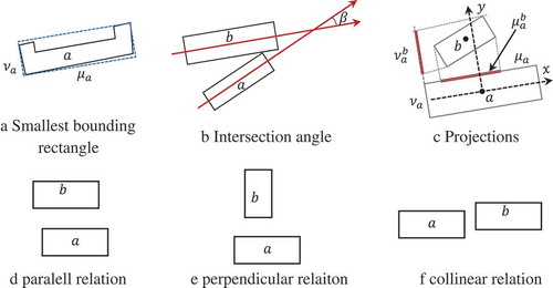
The angle from the $x$ axis to the long axis of $SBR\left(a\right)$ represents the main direction of building $a$. For two buildings $a$ and $b$, if their long axes are parallel and have a large overlapping, they will be parallel (Figure 1d); if their long axes are perpendicular, and the short axis of $b$ is overlapping with the long axis of $a$, they will be perpendicular (Figure 1e); if their long axes are parallel and their short axes are overlapping, they will be collinear (Figure 1f). The detailed definitions of parallel, perpendicular and collinear relations between buildings refer to the work (Du et al. 2016b).

2.2. Fitting degrees of SBRs and division of objects

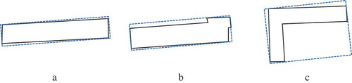
Objects can have any shapes, but SBRs can only fit the objects with simple shapes well, instead of those with complex shapes. Accordingly, an indicator is needed to measure how well a SBR to fit an arbitrary object.

To measure the fitting degree of a SBR to an object, the ratio of the object’s area to its SBR’s area is used (Eq. 1).

(1) $SBR\mathrm{\_}Fitting\left(a\right)=area\left(a\right)/area\left(SBR\left(a\right)\right)$(1)

The range of $SBR\mathrm{\_}Fitting\left(a\right)$ is (0, 1]. Generally, the larger the fitting degree, the better the SBR fits the object. For example, the fitting degrees of the objects in (Figures 2a and 2b) are very large, while the one in (Figure 2c) is small. For the object with a small fitting degree, it should be split into several sub-objects such that the fitting degree of each sub-object is large.

Figure 2. Fitting degree of SBR.

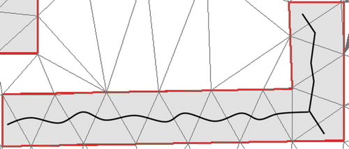
The decomposition of an object with complex shapes can be conducted with the help of triangles and consists of three main steps (Ai and Zhang 2007). First, the constrained Delaunay tri-angulation method is used to partition polygons into triangles because this method can generate triangles with the properties of “as equilateral as possible” avoiding the appearance of very narrow triangles or very sharp angle. Therefore, an object can be represented as a set of triangles as shown in (Figure 3). Second, the skeleton of the object can be generated by linking the midpoint of each triangle edge or the barycenter of each triangle. Finally, the object can be decomposed into sub-objects according to the branches of the skeleton. That is, an object is split into sub-objects in terms of the directions of branches. For example, the object in (Figure 3) will be decomposed into two sub-objects. Once an object is discomposed, the sub-objects will be used as building blocks to model relational contexts.

Figure 3. Fitting degree of SBR, where the black line is the skeleton of the polygon.

3. Relational contexts among buildings

In VHR images, classification errors frequently occur due to large heterogeneity within classes and homogeneity between classes. Heterogeneity within classes implies that visual features vary greatly for the same class of objects due to various imaging conditions and materials. Homogeneity between classes refers to that some objects of different classes may share similar visual features. Accordingly, it is very hard to improve classification accuracy solely by considering visual features. Relational contexts can provide local environments for correcting errors in an initial classification.

This section provides a complete typology of relational contexts and their definitions, such as adjacent, azimuth, alongess, betweenness, among and surrounding relations. These relations can model relational contexts for identifying local environment.

3.1. Adjacent relation

Adjacent relations are crucial to image understanding as most image process operators are suitable only for adjacent objects. Since adjacent relations depend on the shapes of objects which vary greatly in VHR images, Delaunay triangulation of objects are used to define adjacent relations. Two objects $a$ and $b$ are adjacent if they are connected by triangles and denoted by $Adj\left(a,b\right)$. A set of objects $A={\left\{a_i\right\}}_{i=2}^n$ is connected if for any pair of objects $a_i$ and $a_j$ there exists a subset $\left\{a_l,\dots ,a_m\right\}$ in $A$ such that $Adj\left(a_i,a_l\right)\wedge \dots \wedge Adj\left(a_m,a_j\right)$ holds.

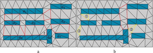
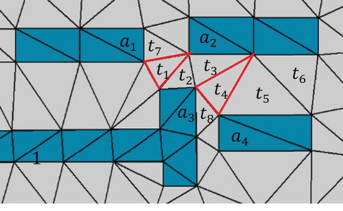
For example, in (Figure 4a), polygon $a_1$ has four neighbors $a_2$, $a_3$, $a_5$ and $a_6$ as they are directly linked with $a_1$ by triangles. Polygons $a_2$ and $a_6$ are not adjacent, while polygons $a_2$, $a_3$ and $a_6$ constitute a connected set. Accordingly, two subsets $\left\{a_2,a_3,a_6\right\}$ and $\left\{a_1,a_5\right\}$ can be regarded as two neighboring wholes and two kinds of relations can be defined: those between the two wholes and those between their components. When grouping polygons into wholes, the sizes are also important. For parallel polygons, their sizes should be similar. For example, polygons $a_1$ and $a_2$ cannot be grouped into a whole as their sizes are greatly different. However, the group $\left\{a_2,a_3\right\}$ and $a_1$ can be parallel as they have similar sizes. Generally, for parallel polygons, they should have large overlapping on their long axes, while for two collinear polygons they should have large overlapping on their short axes; otherwise, they cannot be grouped together.

Figure 4. Delaunay triangulation of buildings, where the red polygons enclose the between/among regions and the yellow polygons refers to the types of triangles (modified from Du et al. 2016b).

3.2. Azimuth relation

Azimuth is a kind of angle measurement to describe the relative position from a target to a referent in a certain direction. For example, shadows are always located in a certain direction relative to buildings, thus this cue help to identify buildings according to shadows, or to identify shadows according to buildings. For example, Zhang et al. (2017b) used shadows and azimuth to identify mid-rise or taller buildings from medium resolution images.

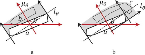
Let $\theta$ be an azimuth angle relative to the horizontal axis and $a$ be a referent, then $AziExt\left(a,\theta \right)$ refers to the spatial region determined by the azimuth angle $\theta$ with respect to referent $a$. Let ${\mu }_{\theta }$ be the line whose inclination angle is $\theta$, and $l_{\theta }$ be the line perpendicular to ${\mu }_{\theta }$, then $AziExt\left(a,\theta \right)$ is defined as the unbounded region formed by the referent $a$ and the two lines through the two end-points of the referent’s projection onto line $l_{\theta }$ and parallel with line ${\mu }_{\theta }$ (i.e. the shadow region in (Figure 5)).

Figure 5. Spatial regions of azimuth relations.

Based on $AziExt\left(a,\theta \right)$, the azimuth relation of target $b$ relative to referent $a$ in the direction $\theta$ can be defined as:

(2) $\begin{array}{c}AziRel\left(a,b,\theta \right){=}_{def}Overlapping\left(AziExt\left(a,\theta \right),b\right)\\ Overlapping\left(a,b\right)=area\left(a\cap b\right)/area\left(b\right)>\delta \end{array}$(2)

In Eq. (2), symbol ${=}_{def}$ means that relation $AziRel\left(a,b,\theta \right)$ holds if only the right part is true. $\delta \in \left[0,1\right]$ is a threshold specified by users. This equation indicates that if target $b$ has a large overlapping with the azimuth region defined by angle $\theta$ and referent $a$, it should be located in the direction $\theta$ of referent $a$. Accordingly, those objects in the azimuth angle of a referent can be determined by Eq. (2).

3.3. Alongness

Alongness relation represents the information on how target $b$ is along referent $a$. This relation between objects $a$ and $b$ holds if the following conditions hold: (1) the visible boundary of target $b$ from referent $a$, denoted by $V\left(a,b\right)$, takes a large part of the boundary of $b$; and (2) the distance between the two objects is small relative to their sizes. The visible boundary of target $b$ with respect to referent $a$ is defined as the boundary points of $b$ from which the shortest distances to the boundary of $a$ is smaller than a threshold.

(3) $Alongness\left(a,b\right){=}_{def}\{V\left(a,b\right)/L\left(b\right)>\lambda \}\wedge \{\left(dist\left(a,b\right)/min\left(area\left(a\right),area\left(b\right)\right)\right)<\delta \}$(3)

where $\lambda \in \left[0,1\right]$ and$\delta \in \left[0,1\right]$ are two thresholds specified by users, and $L\left(b\right)$ refers to the length of $b$’s entire boundary.

In (Figure 6), targets $c$ and $d$ is along referent $a$, while $b$ is not because the visible boundary of $b$ is too small.

Figure 6. Spatial regions of alongness relations.

3.4. Betweeness and among

The betweeness/among relation first uses more than one referents to define a between/among region covering the empty space between/among the referents, and then the relations of a target with respect to the referents can be defined in terms of the relations between the target and the between/among region. Accordingly, the definitions of the between/among regions with respect to the referents are the key to the betweeness/among relations. Because the triangles covering the space between the referents are adaptive to the referents’ shapes and the space between the referents, thus they are used to obtain the between/among regions.

3.4.1. Betweeness

Betweeness is a ternary relation, thus two adjacent objects are considered as the referents and the target should be between the two referents. Let $a_1$ and $a_2$ be the referents, then they define a between region $BetExt\left(a_1,a_2\right)$, which depends on the distance, overlapping rate and adjacent relations. Accordingly, it can be defined in terms of the following rules.

• If two adjacent objects have large overlapping rate among their short or long axes, they can define a between region. For example, in (Figure 4a), objects $a_1$ and $a_2$ can define a between region, while objects $a_2$ and $a_5$ cannot define a between region as they are not neighbors. Similarly, objects $a_3$ and $a_5$ as well as $a_1$ and $a_6$ also cannot define between regions because they are not overlapping on their axes.

• More than two objects can also define a between region if they can be grouped into together. For example, in (Figure 4a), objects $a_2$ and $a_3$ can be grouped together to form a new object $a=a_2{\cup }^{a_3}{\cup }^{B}BetExt\left(a_2,a_3\right)$, then the new object $a$ and $a_4$ are neighbors that can define a new between region $BetExt\left(a,a_4\right)$ again. Accordingly, between regions can be hierarchically defined.

• Two adjacent objects can be perpendicular, parallel and collinear relations (Du, Shu, and Feng 2016a; Du et al. 2016b). Generally, for two collinear objects (e.g. the two objects $a_2$ and $a_3$ in (Figure4a)), their between region links the short axes of their SBRs together; for two parallel objects like the objects {$a_2$, $a_3$} and $a_1$ in (Figure 4a), their between region links the long axes together; while for two perpendicular objects like objects $a_7$ and $a_8$ in (Figure 4a), their between region links their short and long axes together.

The triangles linking adjacent objects can fall into three types in terms of the relations between the triangles and the objects (Figure 4b): ① the three nodes lie on two objects; ② the three nodes lie on three objects respectively; ③ the three nodes lie on two objects and the boundary of the study region. For two objects $a_1$ and $a_2$, the first type of triangles are denoted by $T_1\left(a_1,a_2\right)$.

Visually and cognitively, the between region of two objects $a$ and $b$ can be only composed of the first type of triangles (Eq. 4).

(4) $BetExt\left(a_1,a_2\right)=\left\{t_i|t_i\in T_1\left(a_1,a_2\right)\right\}$(4)

The relative position can also affect the definition of the between region. When object $b$ is perpendicularly adjacent to object $a$, they can define a between region by Eq. (4) if and only if the short axis of $b$ has a large overlapping rate with the long axis of $a$ (Eq. 5).

(5) $Pro\mathrm{\_}Over\left(a,b\right)=\nu {\mu }_a^b/{\nu }_b$(5)

In Eq. 5, $\nu {\mu }_a^b$ refers to the length of the projection of the short axis of target $b$ on the long axis of referent $a$, while ${\nu }_b$ denotes the length of the short axis of target $b$ (Figure 1). For example, in (Figure 4a), objects $a_6$ and $a_8$ cannot define a between region, while $a_7$ and $a_8$ can.

Similar to azimuth relation, the between relation of target $b$ relative to two referents $a_1$ and $a_2$ can be defined in terms of the overlapping ratio between target $b$ and the between region $BetExt\left(a_1,a_2\right)$.

(6) $BetRel\left(a_1,a_2,b\right)={}_{def}Overlapping\left(BetExt\left(a_1,a_2\right),b\right)$(6)

3.4.2. Among

Among relation is a multinary relation because multiple objects are considered as the referents, and the target should be among the referents. Let $A={\left\{a_i\right\}}_{i=3}^n$ be the referents, then these referents can define a among region $AmExt\left(A\right)$. The among region $AmExt\left(A\right)$ can be defined and obtained by an iterative process. First, the among region $AmExt\left(A\right)$ is initialized as a set of the triangles linking three referents in $A$. Second, other triangles should be added to the among region $AmExt\left(A\right)$ if they: (1) link two referents $a_i$ and $a_j$ in $A$; (2) do not belong to the between regions of any other referents in $A$; (3) share one side with the triangles in $AmExt\left(A\right)$; and (4) if $a_i$ is perpendicular to $a_j$ and the short axis of $a_i$ does not have large overlapping rate with the long axis of $a_j$ (Eq. 5), the triangles with two nodes on $a_j$ cannot belong to $AmExt\left(A\right)$. Note that the second step can be repeated many times until there has no triangles satisfying the four conditions.

For example, in (Figure 7), the among region $AmExt\left(\left\{a_1,a_2,a_3\right\}\right)=\left\{t_1,t_2\right\}$. First, the triangle $t_1$ is initially added to the among region; second, $t_2$ is added while $t_3$ and $t_7$ are not. It is clear that $a_3$ is perpendicular to $a_2$ and do not have overlapping, as well as the two nodes of $t_3$ lie on the boundary of $a_2$, thus $t_3$ cannot be included. Similarly, the among region $AmExt\left(\left\{a_2,a_3,a_4\right\}\right)=\left\{t_3,t_4,t_5,t_6\right\}$. First, the triangle $t_4$ is added to the among region as its three nodes link the three polygons; second, the other three triangles are added iteratively as they share nodes with the triangles in $AmExt\left(\left\{a_2,a_3,a_4\right\}\right)$. The triangle $t_8$ is not included because it does not satisfying the fourth condition in define among region.

Figure 7. The among regions, while the red triagnles refer to the first one to be added into the among region.

Similar to the azimuth relation, the among relation of target $b$ relative to referent $A$ can be defined by Eq. (7).

(7) $AmRel\left(A,b\right)={}_{def}Overlapping\left(AmExt\left(A\right),b\right)$(7)

3.5. Surrounding relation

The between and among relations can locate the targets with respect to the regions created by two or more referents, while the surrounding relation can locate objects within the concave parts of a referent. As shown in (Figure 8a), target $b$ is surrounded by referent $a_3$ which consists of three components $a_{31}$, $a_{32}$ and $a_{33}$.

Figure 8. The surrounding regions, where the yellow polygons refer to the surrounding regions, while the red polygon refers to the among region.

To formalize surrounding relations, a surrounding region needs to be defined for a referent. The surrounding region of a referent $a$, denoted by $SurExt\left(a\right)$, is composed of the triangles which link the referent itself but are not within the referent. In (Figure 8a), there is one surrounding region $s$ defined by the referent $a_3$, while in (Figure 8b) the referent $a_3$ corresponds to three surrounding regions $s_1$, $s_2$ and $s_3$.

Similar to the azimuth relation, the surrounding relation of target $b$ relative to referent $a$ can be defined by Eq. (8).

(8) $SurRel\left(a,b\right)={}_{def}Overlapping\left(SurExt\left(a\right),b\right)$(8)

Note that the surrounding relations are only relevant to the objects with complex shapes, i.e., objects with concave parts. The objects with simple shapes are not suitable to define surrounding regions, such as objects $a_1$ and $a_2$ in (Figure 8).

3.6. Relational contexts and their combinations

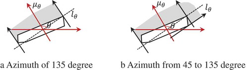
The alongness and azimuth relations can be combined to describe more complicated semantics.

(9) $BuiAlong\left(a,b\right)\wedge DirLocate\left(a,b,\theta \right)$(9)

As shown in (Figure 9), object $b$ is along object $a$ in the direction of 135 degree (Figure 9a), while object $c$ is along object $a$ in the direction from 45 to 135 degree (Figure 9b).

Figure 9. Combination of alongness and azimuth relations.

4. Classifying VHR images with relational contexts

Without relational contexts, the classifier will be applied to choose the labels for all image objects from all classes. Accordingly, the classifier has to predict one class for each object. The accuracy is often not satisfactory because the strong intra-class variation and inter-class confusion of visual features. However, the relational contexts are helpful to identify those objects which belong to a limited set classes instead of all classes and further adopt different classifiers to the objects determined by different relational contexts.

4.1. Methods

Different relational contexts can help to identify different subsets of image objects for two purposes. First, a classifier can work on the chosen subsets of image objects instead of all image objects, thus it could be possible that different classifiers or different parameters, instead of one classifier with the same parameters, can be trained for different subsets. Second, the chosen subsets can belong to limited classes instead of all classes. For example, the image objects between two buildings can be grass, shadows, small trees, or impervious surfaces, but not forest and roads. This helps to improve classification results.

However, for the better use of relational contexts, the initial classification of VHR images is required because the relation contexts depend on both geometries and classes of image objects.

1. Initially classifying VHR images. VHR images are first segmented with the multi-resolution segmentation algorithm, and then all segments are classified using a classifier (SVM, random forest, etc.). Although the accuracy of the initial classification may be not satisfactory, it can be the basis for defining relational contexts to further improve classification accuracy.

2. Extracting building patterns. Groups of buildings in the initial classification results often exhibit collectively some special arrangements termed as collinear and parallel patterns. The relational contexts can be defined on two single buildings or two building patterns. Accordingly, various types of building patterns should be extracted and used for modelling relational contexts. Generally, four types of patterns (collinear, parallel, perpendicular and grid patterns) are obtained with the relational approach (Du, Shu, and Feng 2016a; Du et al. 2016b).

3. Identifying subsets of segments with relational contexts. In Section 3, adjacent relation, alongness, betweenness, among, and surrounding relations are formalized from a geometric view. However, these relations can describe the relational semantics about different classes, thus the relations between different classes should be considered. Buildings are the crucial class of man-made objects in urban areas, and other classes have strong correlations with buildings. Accordingly, the patterns about buildings can be used to define the relational contexts in Section 3, which are further used for improving the initial classification by correcting classes for misclassified segments.

4. Correcting classification errors with relational contexts. Using the relational contexts and semantic classes of objects, the objects of interesting can be chosen for correcting misclassification in initial classification results.

Through the four steps above, visual features and relational contexts can be combined to classify VHR images with a large accuracy. The first two steps are already resolved and the details refer to the related references, while the latter two will be detailed in the following two sections.

4.2. Identifying objects with relational contexts

Relational contexts can help to identify objects in a local environment. For example, relation $AziRel\left(a,b,\theta \right)$ can identify two lists of objects overlapping with the azimuth region of referent $a$ (Eq. 10).

(10) $\begin{array}{c}Azi\mathrm{\_}List\left(a,\theta \right)=\left\{b|AziRel\left(a,b,\theta \right)\right\}\\ Azi\mathrm{\_}List\left(a,\theta ,d\right)=\left\{b|AziRel\left(a,b,\theta \right)\wedge distance\left(a,b\right)<\sigma \right\}\end{array}$(10)

where $distance\left(a,b\right)$ refers to the distance between objects $a$ and $b$ and $\sigma$ is a threshold specified by users. $Azi\mathrm{\_}List\left(a,\theta \right)$ refers to all objects located in the direction $\theta$ of referent $a$, while $Azi\mathrm{\_}List\left(a,\theta ,d\right)$ includes all objects located in the direction $\theta$ of referent $a$, but also the distance from target $b$ to referent $a$ is smaller than the threshold $\sigma$. Similarly, other relational contexts can also be used to define the lists for further analysis.

4.3. Correcting objects’ classes

The correction of misclassified objects can be conducted based on the relational contexts. Those objects identified by relational contexts can be reclassified by a ruleset designed by users or a new classifier which can have different parameters or different forms from the original one. In this case, new samples should be chosen for training a new classifier. Finally, the trained new classifier can be used to reclassify those objects identified by the relational contexts. In different cases, different relational contexts can be used to identify candidates.

5. Test data and processing methods

5.1. Data

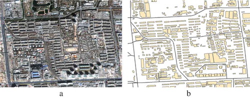
A Quickbird image subset (Figure 10a) acquired in 2002 and a vector dataset of roads and buildings (Figure 10b) were used as experimental data to test the presented approach, and they cover a block of the urban area in Beijing city, China. The resolution is 0.6 m for the panchromatic channel and 2.4 m for the multispectral channels. The vector dataset consists of 475 buildings and eight major roads, and covers the same area with the Quickbird image. Since GIS data are crucial to urban transportation, many commercial companies, government departments and volunteers collect and update these data. As a result, building and road data, are easily available for common cities, such as VGI data. Hence, such data can be used to extract relational contexts because the initial classification results may contain errors, which may influence the extraction of relational contexts.

Figure 10. Test data. (a) Quickbird image in Beijing city and (b) existing vector buildings and roads.

5.2. Processing methods

To obtain the initial classification results, GEOBIA techniques are used. Five steps are included and detailed as follows.

1. Data preprocessing. The original five bands of the Quickbird image were merged using the pan-sharpening procedure (Laben and Brower 2000) in ENVI to produce a fused image with a spatial resolution of 0.61 m and four multispectral bands. The fused image and building vector data were further georeferenced using ArcGIS to reduce distortion between the two data.

2. Image segmentation. The multi-resolution segmentation algorithm (Baatz and Schäpe 2000) was carried out to divide the fused four-band image into multiscale image objects. An optimal scale of 50 was selected using the estimation tool of scale parameter (Drǎguţ, Tiede, and Levick 2010; Drăguţ et al. 2014).

3. Sampling collection. For training a SVM classifier and testing the accuracy of the presented method, the training and testing samples were selected independently and manually based on the segmented objects. Totally, 120 training samples (Figure 11) and 2133 testing samples were selected.

4. Initial classification. The SVM classifier with linear kernel was used to classify the objects by considering visual features and the cross validation method was used to determine the kernel function parameters. Feature selection in this study can be based on either past experience and user knowledge or a feature selection algorithm prior to final classification (Duro, Franklin, and Dubé 2012). In this study, the feature selection is guided by previous studies (e.g. Pu, Landry, and Yu 2011; Du, Zhang, and Zhang 2015) and visual examination. In total, the 23 features (Table 1) were defined and used in the initial classification. The land-cover map consists of six classes: buildings, trees, shadows, roads, water and other surfaces.

5. Building patterns extraction. The relational contexts in Section 3 depend on either single buildings or building patterns, thus building patterns should be first extracted from vector buildings by the extraction methods (Du, Shu, and Feng 2016a; Du et al. 2016b).

6. Relational contexts extraction. The methods in Section 3 are used in this step.

Table 1. The number of training and test samples for each class.

	Buildings	Trees	Shadows	Roads	Water	Other surfaces
Training samples	27	31	20	17	5	20
Test samples	468	598	343	233	24	467

Figure 11. The training samples in the initial classification.

For the former four steps, the tools are available to implement data analysis, while no tools are available for the latter two steps. We have to develop tools for extracting building patterns and relational contexts by using the Visual C++ in Visual Studio 2015 (The source code can be available if readers email us). The reported results in the following sections were obtained by the developed tools.

6. Results and discussion

6.1. Results of relational contexts

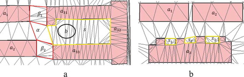
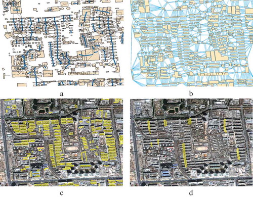
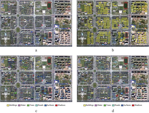
In total, 66 collinear building patterns were obtained (Figure 12a). In this test, two typical relational contexts, namely the betweeness among buildings within building patterns (denoted as $Co{n}_{Bui}^{bet}$, (Figure 12c)) and the betweeness among collinear building patterns (denoted as $Co{n}_{Pat}^{bet}$, (Figure 12d)), were extracted and used as examples. It is clear that betweeness actually define some new regions, which help to choose image objects falling within the betweeness region, denoted by $Bet\mathrm{\_}List\left(a_1,a_2\right)$. A total of 163 betweeness regions between buildings and eight betweeness regions among collinear building patterns are obtained in the experimental image.

Figure 12. Results of extracted relational contexts. (a) Collinear building patterns, (b) the betweeness relations among all buildings, (c) betweeness regions between buildings within building patterns, and (d) betweeness regions among collinear building patterns.

6.2. Results of the initial classification using visual features

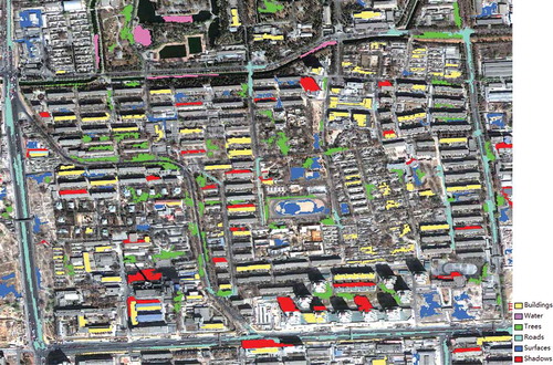
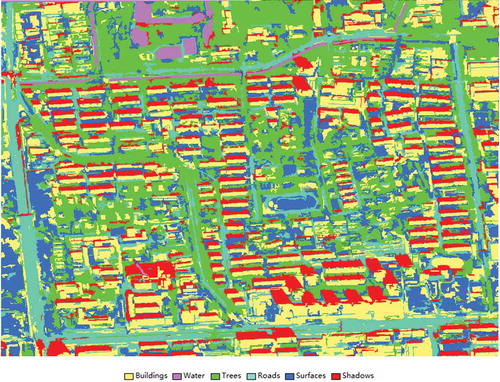
Totally, the fused image was segmented by using the selected optimal scale of 50, and 6256 objects were produced (Figure 13a). (Figure 13b) shows the results of the initial classification.

Figure 13. Results of initial classification. (a) Segmented objects, and (b) classified objects.

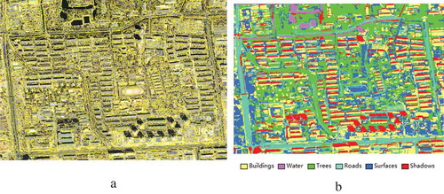
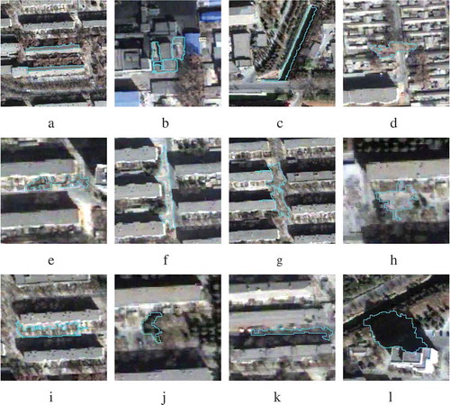
In (Table 3), the initial accuracies (F-Score) of buildings, water, trees, roads, surfaces and shadows are 65.5%, 65.4%, 86.0%, 51.4%, 51.6%, 86.0%, respectively. The overall accuracy for all classes is 69.5% and the kappa coefficient is 61.7%. The relative low accuracies are led by the confusion of visual features. The misclassified classes fall to three groups. The first group includes buildings, roads and other surfaces, which are artificial constructions and very similar in visual features. As a result, it is difficult to distinguish them from each other by only visual features (Figure 14a-b, f-i). The second group refers to water and shadows, which are often confused with each other (Figures 14c and 14l) as they are always similar in color, size and shape. The third confused group includes shadows, trees (Figure 14j) and roads (Figure 14k), because they are dark in some cases. Two reasons can account for this kind of confusion. First, it is hard to separate trees from their shadows during image segmentation, leading to that image objects misclassified, as trees are actually the mixtures of trees and shadows. Second, the Quickbird image used was acquired at the beginning of March, thus the trees are not green in this period.

Table 2. The features used in the initial classification.

Types	Names	Meanings
Spectrum	[Mean]	The average spectrum of pixels
	[Brightness]	The weighted average spectrum of pixels on each band
	[Max. diff.]	The ratio of the maximal difference of average spectrum of each band to the brightness
	[Std. dev]	The standard deviation of pixels’ grayscale of an image object
	[NDVI]	Normalized difference vegetation index
	[Skewness]	The skewness of grayscale histogram of pixels
	[Ratio]	The ratio of average spectrum to brightness
Texture	[Entropy]	The entropy derived from GLCM
	[Dissimilarity]	The heterogeneity derived from GLCM
	[Homogeneity]	The homogeneity derived from GLCM
	[Contrast]	The contrast derived from GLCM
Geometry	[Area]	The number of pixels within image objects
	[Border length]	The number of pixels on the inner and outer borders
	[Length]	The length of the envelop rectangle
	[Width]	The width of the envelop rectangle
	[Length/Width]	The length-width ratio of the envelop rectangle
	[Roundness]	The difference between the radiuses of the maximal inscribed and minimum circumscribed ellipses
	[Elliptic fit]	The goodness of an image object fitting into an ellipse
	[Border index]	The ratio between the border lengths of the image object and the smallest enclosing rectangle
	[Compactness]	The ratio of the product of length and width to the area an image object
	[Main direction]	The direction of the eigenvector belonging to the larger of the two eigenvalues
	[Rectangular fit]	The goodness of an image object fitting into a rectangle
	[Shape index]	The ratio of perimeter of a building to four times the square root of its area

Table 3. Confusion matrix of the initial classification results.

Predicted Actual	Buildings	Water	Trees	Roads	Surfaces	Shadows	F-Score
Buildings	349	0	3	58	54	4	65.5%
Water	0	17	1	0	0	6	65.4%
Trees	9	1	477	40	55	16	86.0%
Roads	55	0	7	148	14	9	51.4%
Surfaces	182	0	5	73	206	1	51.6%
Shadows	3	10	18	24	2	286	86.0%

Figure 14. Examples of misclassified classes. (a) Buildings classified as roads, (b) buildings as surfaces, (c) water as shadows, (d) trees as surfaces, (e) trees as roads, (f) roads as buildings, (g) roads as surfaces, (h) surfaces as buildings, (i) surfaces as roads, (j) shadows as trees, (k) shadows as roads, and (l) shadows as water.

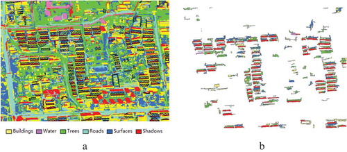
6.3. Results of the post-classification using relational contexts

If only visual features in (Table 2) are used for classification, three groups of misclassified classes could be produced in the initial results. Therefore, relational contexts have to be used as post-classification method to correct the misclassified classes in terms of the following three steps. First, those objects are first identified if they are located in the local regions defined by relational contexts. Second, a new classifier is trained by choosing samples from the identified objects in the first step. Third, the trained classifier is used to re-classify other objects within the local regions.

By overlaying the initial classification results with the relational contexts $Co{n}_{Bui}^{bet}$ (Figure 15a), those objects located in $Co{n}_{Bui}^{bet}$ (Figure 15b) can be determined for re-classification. Totally, 39 training samples were manually selected from those objects located in $Co{n}_{Bui}^{bet}$ and another linear SVM classifier was trained with the samples. Then, all objects in $Co{n}_{Bui}^{bet}$ were reclassified into three classes (i.e., trees, shadow and other surfaces) by the trained classifier. Similarly, only trees, shadows and roads can often appear in the local regions $Co{n}_{Pat}^{bet}$, while other classes can rarely emerge in these areas. Thus, a refined local reclassification was carried out similarly.

Figure 15. Retrieved image objects using relational contexts. (a) Overlay of the initial classification and the relational contexts, and (b) the objects located in the relational contexts.

The azimuth (Section 3.4) and alongness relation (Section 3.5) can help to solve the confusion problem of water and shadows. Actually, shadows always co-exist with buildings in a certain direction related to the sun, while water do not. As a result, the relations, azimuth modelling the sun’s azimuth and alongnness modelling the relations between buildings and shadows, can help to determine whether the image objects are shadows or water (Figure 16a). A total of six water objects in the initial classification results were corrected as shadows, and five shadow objects in the initial classification were reclassified as water. Moreover, the relational contexts azimuth and alongness also reduce the confusion problem of buildings, roads and other surfaces (Figure 16b). A total of 35 road objects and 22 surface objects in the initial classification were reclassified as buildings. The refined classification map is shown in (Figure 17).

Figure 16. Azimuth and alongness relations for distinguishing water and shadows.

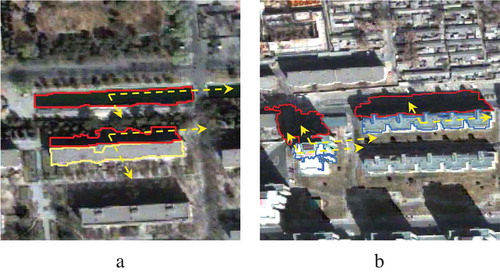
Figure 17. The refined results of post-processing.

To verify the results in detail, accuracy evaluation was carried out by using confusion matrix. The confusion matrix of the refined classifications is shown in (Table 4).

Table 4. Confusion matrix of refined classification.

Predicted Actual	Buildings	Water	Trees	Roads	Surfaces	Shadows	F-Score
Buildings	406	0	3	23	32	4	82.9%
Water	0	23	1	0	0	0	95.8%
Trees	1	1	533	7	48	8	92.9%
Roads	46	0	4	167	7	9	72.9%
Surfaces	56	0	2	20	388	1	82.1%
Shadows	2	0	7	8	3	323	93.9%

In (Table 4), the refined classification accuracies (F-Score) of buildings, water, trees, roads, surfaces and shadows are 82.9%, 95.8%, 92.9%, 72.9%, 82.1%, 93.9%, respectively. The overall accuracy is 86.3% and the kappa coefficient is 82.6%. Apparently, the refined accuracies are greatly improved from those in (Table 3). The improvements of the six classes are 17.5%, 30.4%, 6.8%, 21.5%, 30.5%, and 7.9%, respectively. This is largely due to less confusing categories and better sample selection in the local areas defined by relational contexts.

6.4. Testing on one more data

To verify genericity of the proposed method, another dataset acquired in 2016 from the GF-2 satellite was tested. A fused image (Figure 19a) was used as experimental data, which has a spatial resolution of 0.81 meter and consists of four spectral bands, covering a block of the urban area in Bengbu city, China. In total, 280 betweeness regions (Figure 19b) were obtained as relational contexts. After the post-classification process, the classification results of 226 image objects have been corrected. (Figure 19c) and (Figure 19d) show the differences.

Figure 18. A map of differences between (a) the initial results and (b) the refined results.

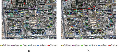
Figure 19. The test on GF-2 data. (a) The experimental image, (b) betweeness regions between buildings within building patterns, (c) the reclassified objects in the post-classification, and (d) the same objects in (c) in the initial classification.

The test on GF-2 data. (a) The experimental image, (b) betweeness regions between buildings within building patterns, (c) the reclassified objects in the post-classification, and (d) the same objects in (c) in the initial classification.

The confusion matrices of the initial and refined classification results are shown in (Table 5) and (Table 6), respectively. After the post-classification process, the overall accuracy increases from 65.4% to 90.8%, and the kappa coefficient increases from 57.1% to 88.5%. The improvements of the six classes are 28.1%, 88.0%, 16.5%, 16.3%, 40.0% and 17.5%, respectively. This demonstrates that the proposed method is also promising for this data. Therefore, this method has stronger genericity and practicability. The initial accuracy of water is zero (Table 5) due to the few number of water objects and the confusion of water and shadow objects in the study area.

Table 5. Confusion matrix of initial classification results using GF-2 data.

Predicted Actual	Buildings	Water	Trees	Roads	Surfaces	Shadows	F-Score
Buildings	152	0	2	33	5	6	61.7%
Water	1	0	2	0	0	11	0
Trees	32	1	130	6	8	0	81.5%
Roads	4	0	1	98	1	0	62.4%
Surfaces	71	1	4	70	74	0	48.1%
Shadows	35	0	3	3	0	113	79.6%

Table 6. Confusion matrix of refined classification results by relational contexts.

Predicted Actual	Buildings	Water	Trees	Roads	Surfaces	Shadows	F-Score
Buildings	171	0	2	11	8	6	89.8%
Water	1	11	1	0	0	1	88.0%
Trees	1	0	174	1	1	0	98.0%
Roads	4	0	1	98	1	0	78.7%
Surfaces	4	0	0	35	181	0	88.1%
Shadows	2	0	0	0	0	152	97.1%

6.5. Comparison with CRF model

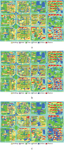
A comparative study with the conditional random field (CRF) was also investigated. The initial classification results (Figure 20a) are individually refined by a CRF model integrating spectral, spatial context, and spatial location cues (Zhao et al. 2016). With regard to the CRF-refined classification results (Figure 20c), the overall accuracy is 71.0% and the kappa coefficient is 63.9% (derived from Table 7), which are much smaller than that of the presented approach. By comparing the performances of our method and the CRF model for post-classification, it can be seen that relational contexts approach achieves the higher accuracy. Although the CRF approach could correct some mistakes in the initial classifications, it would also bring many new misclassifications. For example, in this test, the classification accuracy of other surfaces is greatly improved by the CRF model, while many objects that were correctly classified as shadows in the initial classification were mistaken by the CRF in the meantime. By contrast, there would be few such problems for the relational contexts approach, since the refinement of the classification results are only conducted in the local areas defined by relational contexts.

Table 7. Confusion matrix of refined classification results by the CRF model.

Predicted Actual	Buildings	Water	Trees	Roads	Surfaces	Shadows	F-Score
Buildings	168	0	2	16	7	5	68.2%
Water	2	6	2	0	0	4	57.1%
Trees	22	0	130	6	18	1	81.3%
Roads	5	0	2	95	2	0	71.2%
Surfaces	63	1	6	42	105	3	59.3%
Shadows	35	0	1	4	2	112	80.3%

Figure 20. The classification results. (a) The initial results, (b) the results refined with relational contexts, and (c) the CRF-refined classification results.

6.6. Discussion

The test results demontrate that the post-classification using relational contexts produced more precise results than the initial classification. The relational contexts define the local environments to further distinguish objects in the following two ways. First, the relational contexts can narrow the search space and classes. That is, only parts of objects need to be classified and part of classes needs to be considered. The relational contexts can help to determine the part of objects and recognize the part of classes. For example, only three classes (i.e., trees, shadows and impervious surfaces) are possible for those objects located in the local regions between buildings, while other classes could rarely happen. Second, for a supervised classification process, the selected samples and trained classifiers have great influences on classification accuracy. Normally, the samples are selected from the whole image and one classifier is trained for handling all image objects. The relational contexts can help to select multiple sets of samples and to train multiple classifiers in the local environments, which would be beneficial to improve image classification. In one word, the relational contexts provide local environments and a potential for refining those image objects that are misclassified by a global classifier. Accordingly, the relational contexts in this study are good complements to existing three strategies for modelling contexts, including random field model (Moser and Serpico 2013; Zhang et al. 2017a), multi-level features (Bruzzone and Carlin 2006), and class-related features in GEOBIA framework (Trimble 2011). The reason is that the latter three strategies actually do not model spatial relations and cannot provide the local environments for improving land-cover mapping.

In this study, the relational contexts are extracted from buildings vector data, which sometimes are not available. Therefore, the best way is to extract contexts from initial classification results using an object-based classifier. This inevitably brings some initial classification errors into the extraction of relational indices. How to overcome this issue will be future research topic. The relational contexts are helpful to interpreting VHR images more accurately, but they may not be much useful to medium resolution images as individual buildings are difficult to identify. However, other post-classification methods are applicable to medium resolution images. For example, the Markov chain random field cosimulation (Li et al. 2015) was used in detecting urban vertical growth from medium resolution images recently (Zhang et al. 2017b, 2018).

In supervised classification, the state-of-the-art accuracy can be achieved, but this depends on the try-and-error methods and careful choice on large number of training samples. The determination of classifier parameters and the selection of samples always have to be well-designed, which obviously needs a great effort. On the contrary, we provide a relatively simple way for improving the initial classification, in which a simple classifier is used and dozens of samples are enough. A low initial accuracy may be produced in some degree, but our approach still can make up this shortage and high accuracy can still be achieved. In our approach, the whole process for extracting relational contexts is mainly automated, thus it can be done in a very short time. Besides, the refined classification is conducted locally rather than globally, so it can also be completed quickly.

7. Conclusions

Since visual features on VHR images show large variations within classes and small variations between classes in urban areas, there is still room for improving the accuracy of urban land-cover mapping with VHR images. This study presents the approaches for modelling the relational contexts as human beings often use spatial relationships and spatial reasoning to obtain satisfactory results when they visually interpret VHR images. The involved relational contexts include alongness, betweeness, among, surrounding, and azimuth relations, as well as the combinations of these relations. The presented contexts are first formalized, and then incorporated into a post-classification process. The experimental results with VHR images demonstrate that the relational contexts can improve the classification accuracies of buildings, water, trees, roads, impervious surfaces and shadows by 12.2%, 25%, 9.3%, 8.2%, 39% and 10.2%, respectively. The future work will focus on the roles of the relational contexts in remote sensing interpretation, change detection, and image matching.

Acknowledgements

The work presented in this paper was supported by the National Natural Science Foundation of China (No. 41471315).

Disclosure statement

No potential conflict of interest was reported by the authors.

Additional information

Funding

This work was supported by the National Natural Science Foundation of China [41471315];

References

- Ai, T., and X. Zhang. 2007. “The Aggregation of Urban Building Clusters Based on the Skeleton Partitioning of Gap Space.” In: The European Information Society: Leading the Way with Geo-Information (AGILE07), Lecture Notes in Geoinformation and Cartography, eds S. I. Fabrikant and M. Wachowicz, 153–170. Aalborg, Denmark: Springer.
- Baatz, M., and A. Schäpe. 2000. “Multiresolution Segmentation: An Optimization Approach for High Quality Multi-Scale Image Segmentation.” Angewandte Geographische Informationsverarbeitung XII: 12–23.
- Blaschke, T., et al. 2014. “Geographic Object-based Image Analysis - Towards a New Paradigm.” Isprs Journal Of Photogrammetry and Remote Sensing 87 :180–191. doi: 10.1016/j.isprsjprs.2013.09.014.
- Bruzzone, L., and L. Carlin. 2006. “A Multilevel Context-Based System for Classification of Very High Spatial Resolution Images.” IEEE Transactions on Geoscience and Remote Sensing 44 (9): 2587–2600. doi:10.1109/TGRS.2006.875360.
- Cohn, A. G., and J. Renz. 2007. “Qualitative Spatial Representation and Reasoning.” In: Handbook of Knowledge Representation, edited by B. Porter, 551–596, Amsterdam, Netherlands: Elsevier.
- Datcu, M., H. Daschiel, A. Pelizzari, M. Quartulli, A. Galoppo, A. Colapicchioni, M. Pastori, K. Seidel, P. G. Marchetti, and S. D’Elia. 2003. “Information Mining in Remote Sensing Image Archives: System Concepts.” IEEE Transactions on Geoscience and Remote Sensing 41 (12): 2923–2936. doi:10.1109/TGRS.2003.817197.
- Drǎguţ, L., D. Tiede, and S. R. Levick. 2010. “ESP: A Tool to Estimate Scale Parameter for Multiresolution Image Segmentation of Remotely Sensed Data.” International Journal of Geographical Information Science 24 (6): 859–871. doi:10.1080/13658810903174803.
- Drăguţ, L., O. Csillik, C. Eisank, and D. Tiede. 2014. “Automated Parameterisation for Multi-Scale Image Segmentation on Multiple Layers.” ISPRS Journal of Photogrammetry and Remote Sensing 88: 119–127. doi:10.1016/j.isprsjprs.2013.11.018.
- Du, S., F. Zhang, and X. Zhang. 2015. “Semantic Classification of Urban Buildings Combining VHR Image and GIS Data: An Improved Random Forest Approach.” ISPRS Journal of Photogrammetry and Remote Sensing 105: 107–109. doi:10.1016/j.isprsjprs.2015.03.011.
- Du, S., L. Luo, K. Cao, and M. Shu. 2016b. “Extracting Building Patterns with Multilevel Graph Partition and Building Grouping.” ISPRS Journal of Photogrammetry and Remote Sensing 122: 81–96. doi:10.1016/j.isprsjprs.2016.10.001.
- Du, S., M. Shu, and -C.-C. Feng. 2016a. “Representation and Discovery of Building Patterns: A Three-Level Relational Approach.” International Journal of Geographic Information Science 30 (6): 1161–1186. doi:10.1080/13658816.2015.1108421.
- Duro, D. C., S. E. Franklin, and M. G. Dubé. 2012. “A Comparison of Pixel-Based and Object-Based Image Analysis with Selected Machine Learning Algorithms for the Classification of Agricultural Landscapes Using SPOT-5 HRG Imagery.” Remote Sensing of Environment 118: 259–272. doi:10.1016/j.rse.2011.11.020.
- Egenhofer, M. J., and J. R. Herring, 1991. “Categorizing Binary Topological Relations between Regions, Lines and Points in Geographic Databases.” Technical Report, Orono, USA: Department of Surveying Engineering, University of Maine.
- Frank, A. U. 1996. “Qualitative Spatial Reasoning: Cardinal Directions as an Example.” International Journal of Geographical Information Science 10 (3): 269–290. doi:10.1080/02693799608902079.
- Goyal, R. K., 2000. “Similarity assessment for cardinal directions between extended spatial objects.” PhD diss., University of Maine.
- Hermosilla, T., L. A. Ruiz, J. A. Recio, and M. Cambra-López. 2012. “Assessing Contextual Descriptive Features for Plot-Based Classification of Urban Areas.” Landscape and Urban Planning 106 (1): 124–137. doi:10.1016/j.landurbplan.2012.02.008.
- Huang, X., Q. Lu, L. Zhang, and A. Plaza. 2014. “New Postprocessing Methods for Remote Sensing Image Classification: A Systematic Study. .” IEEE Transactions on Geoscience and Remote Sensing 52 (11): 7140–7159. doi:10.1109/TGRS.2014.2308192.
- Hussain, M., D. Chen, A. Cheng, H. Wei, and D. Stanley. 2013. “Change Detection from Remotely Sensed Images: From Pixel-Based to Object-Based Approaches.” ISPRS Journal of Photogrammetry and Remote Sensing 80: 91–106. doi:10.1016/j.isprsjprs.2013.03.006.
- Laben, C. A., and B. V. Brower. 2000. Process for Enhancing the Spatial Resolution of Multispectral Imagery Using Pan-Sharpening. US Patent 6,011,875.
- Leinenkugel, P., T. Esch, and C. Kuenzer. 2011. “Settlement Detection and Impervious Surface Estimation in the Mekong Delta Using Optical and SAR Remote Sensing Data.” Remote Sensing of Environment 115 (12): 3007–3019. doi:10.1016/j.rse.2011.06.004.
- Li, W., C. Zhang, M. R. Willig, D. K. Dey, G. Wang, and L. You. 2015. “Bayesian Markov Chain Random Field Cosimulation for Improving Land Cover Classification Accuracy.” Mathematical Geosciences 47 (2): 123–148. doi:10.1007/s11004-014-9553-y.
- Manandhar, R., I. O. A. Odeh, and T. Ancev. 2009. “Improving the Accuracy of Land Use and Land Cover Classification of Landsat Data Using Post-Classification Enhancement.” Remote Sensing 1: 330–344. doi:10.3390/rs1030330.
- Moser, G., and S. B. Serpico. 2013. “Combining Support Vector Machines and Markov Random Fields in an Integrated Framework for Contextual Image Classification.” IEEE Transactions on Geoscience and Remote Sensing 51 (5): 2734–2752. doi:10.1109/TGRS.2012.2211882.
- Myint, S. W., P. Gober, A. Brazel, S. Grossman-Clarke, and Q. Weng. 2011. “Per-Pixel Vs. Object-Based Classification of Urban Land Cover Extraction Using High Spatial Resolution Imagery.” Remote Sensing of Environment 115: 1145–1161. doi:10.1016/j.rse.2010.12.017.
- Pacifici, F., M. Chini, and W. J. Emery. 2009. “A Neural Network Approach Using Multi-Scale Textural Metrics from Very High-Resolution Panchromatic Imagery for Urban Land-Use Classification.” Remote Sensing of Environment 113 (6): 1276–1292. doi:10.1016/j.rse.2009.02.014.
- Pu, R., and S. Landry. 2012. “A Comparative Analysis of High Spatial Resolution IKONOS and WorldView-2 Imagery for Mapping Urban Tree Species.” Remote Sensing of Environment 124 (9): 516–533. doi:10.1016/j.rse.2012.06.011.
- Pu, R., S. Landry, and Q. Yu. 2011. “Object-Based Urban Detailed Land Cover Classification with High Spatial Resolution IKONOS Imagery.” International Journal of Remote Sensing 32 (12): 3285–3308. doi:10.1080/01431161003745657.
- Quartulli, M., and I. G. Olaizola. 2013. “A Review of EO Image Information Mining.” ISPRS Journal of Photogrammetry and Remote Sensing 75 (1): 11–28. doi:10.1016/j.isprsjprs.2012.09.010.
- Sebari, I., and D. C. He. 2013. “Automatic Fuzzy Object-Based Analysis of VHSR Images for Urban Objects Extraction.” ISPRS Journal of Photogrammetry and Remote Sensing 79 (5): 171–184. doi:10.1016/j.isprsjprs.2013.02.006.
- Stuckens, J., P. R. Coppin, and M. E. Bauer. 2000. “Integrating Contextual Information with Per-Pixel Classification for Improved Land Cover Classification.” Remote Sensing of Environment 71 (3): 282–296. doi:10.1016/S0034-4257(99)00083-8.
- Tigges, J., T. Lakes, and P. Hostert. 2013. “Urban Vegetation Classification: Benefits of Multitemporal RapidEye Satellite Data.” Remote Sensing of Environment 136 (5): 66–75. doi:10.1016/j.rse.2013.05.001.
- Trimble. 2011. e-Cognition Developer 8.64.1 User Guide, 250. Germany: Trimble Documentation.
- Voltersen, M., C. Berger, S. Hese, and C. Schmullius. 2014. “Object-Based Land Cover Mapping and Comprehensive Feature Calculation for an Automated Derivation of Urban Structure Types at Block Level.” Remote Sensing of Environment 154: 192–201. doi:10.1016/j.rse.2014.08.024.
- Yue, P., L. Di, Y. Wei, and W. Han. 2013. “Intelligent Services for Discovery of Complex Geospatial Features from Remote Sensing Imagery.” ISPRS Journal of Photogrammetry and Remote Sensing 83 (3): 151–164. doi:10.1016/j.isprsjprs.2013.02.015.
- Zhang, W., W. Li, C. Zhang, D. M. Hanink, Y. Liu, and R. Zhai. 2018. “Analyzing Horizontal and Vertical Urban Expansions in Three East Asian Megacities with the SS-coMCRF Model.” Landscape and Urban Planning 177: 114–127. doi:10.1016/j.landurbplan.2018.04.010.
- Zhang, W., W. Li, C. Zhang, and W. B. Ouimet. 2017b. “Detecting Horizontal and Vertical Urban Growth from Medium Resolution Imagery and Its Relationships with Major Socioeconomic Factors.” International Journal of Remote Sensing 38 (12): 3704–3734. doi:10.1080/01431161.2017.1302113.
- Zhang, W., W. Li, C. Zhang, and X. Li. 2017. “Incorporating Spectral Similarity into Markov Chain Geostatistical Cosimulation for Reducing Smoothing Effect in Land Cover Post-Classification.” IEEE Journal of Selected Topics in Applied Earth Observations and Remote Sensing 10 (3): 1082–1095. doi:10.1109/JSTARS.2016.2596040.
- Zhang, X., and S. Du. 2015. “A Linear Dirichlet Mixture Model for Decomposing Scenes: Application to Analyzing Urban Functional Zonings.” Remote Sensing of Environment 169: 37–49. doi:10.1016/j.rse.2015.07.017.
- Zhao, J., Y. Zhong, H. Shu, and L. Zhang. 2016. “High-Resolution Image Classification Integrating Spectral-Spatial-Location Cues by Conditional Random Fields.” IEEE Transactions on Image Processing 25 (9): 4033–4045. doi:10.1109/TIP.2016.2577886.
- Zhou, W., G. Huang, A. Troy, and M. L. Cadenasso. 2009. “Object-Based Land Cover Classification of Shaded Areas in High Spatial Resolution Imagery of Urban Areas: A Comparison Study.” Remote Sensing of Environment 113 (8): 1769–1777. doi:10.1016/j.rse.2009.04.007.