Vegetation species mapping in a coastal-dune ecosystem using high resolution satellite imagery

Abstract

Vegetation mapping is a priority when managing natural protected areas. In this context, very high resolution satellite remote sensing data can be fundamental in providing accurate vegetation cartography at species level. In this work, a complete processing methodology has been developed and validated in a complex vulnerable coastal-dune ecosystem. Specifically, the analysis has been carried out using WorldView-2 imagery, which offers spatial and spectral resolutions. A thorough assessment of 5 atmospheric correction models has been performed using real reflectance measures from a field radiometry campaign. To select the classification methodology, different strategies have been evaluated, including additional spectral (23 vegetation indices) and spatial (4 texture parameters) information to the multispectral bands. Likewise, the application of linear unmixing techniques has been tested and abundance maps of each plant species have been generated using the library of spectral signatures recorded during the campaign. After the analysis conducted, a new methodology has been proposed based on the use of the 6S atmospheric model and the Support Vector Machine classification algorithm applied to a combination of different spectral and spatial input data. Specifically, an overall accuracy of 88,03% was achieved combining the corrected multispectral bands plus a vegetation index (MSAVI2) and texture information (variance of the first principal component). Furthermore, the methodology has been validated by photointerpretation and 3 plant species achieve significant accuracy: Tamarix canariensis (94,9%), Juncus acutus (85,7%) and Launaea arborescens (62,4%). Finally, the classified procedure comparing maps for different seasons has also shown robustness to changes in the phenological state of the vegetation.

Keywords:

• automatic vegetation classification
• high resolution
• atmospheric correction
• 6S
• Support Vector Machines
• WorldView-2

Introduction

Conservation of the environment is extremely important for human development and well-being. Unfortunately, human activity during the last century has altered it greatly and, as a result, ecosystems are being degraded. Therefore, monitoring natural areas is a priority for organizations responsible for applying management and conservation measures (Isbell, Calcagno, and Hector 2011). In this context, remote sensing is a mature technology at the service of natural resources, providing the largest source of spatial information on the state of conservation and dynamics of ecosystems (Khare and Ghosh 2016).

The launch of new satellites with improved performance and the progress made in processing have allowed the application of remote sensing for the accurate generation of cartographic maps in natural protected areas. In this sense, WorldView satellite series offer spatial resolution and additional spectral bands compared to similar high resolution sensors.

It should be noted that classification of plant species using remote sensing data presents great difficulty in certain ecosystems, such as coastal dunes, due to the small size and density of plants and the complexity and heterogeneity of the existing species (Lu and Weng 2007; Ibarrola-Ulzurrun, Gonzalo-Martín, and Marcello 2017a). Therefore, it is first necessary to carry out a rigorous analysis of the most appropriate image corrections techniques to properly apply the best algorithms. The most representative disturbances to correct are due to the absorption and scattering of the atmosphere. Once data are corrected, remote sensing classification can be applied involving different steps to get the appropriate thematic map. Support Vector Machine (SVM) (Vapnik 1998) has been applied to the problem of classifying because it offers, in general, better or similar results than traditional or advanced methods regardless of the size and quality of the calibration dataset.

The natural area to be studied, the dunes of Maspalomas (Gran Canaria, Spain), is a coastal dune ecosystem. It has undergone significant environmental transformation due to the high anthropogenic pressure that tourism development has caused over the decades (Hernández Calvento 2006; Cabrera Vega et al. 2013; Hernández-Calvento et al. 2014; Hernández- Cordero, Hernández-Calvento, and Pérez-Chacón 2017).

In this context, in the study of the spatio-temporal evolution of plant communities, it is important to analyze the changes experienced by this system of dunes, and other similar ones around the world, since this type of ecosystems has a close relationship between vegetation and aeolian sedimentary dynamics.

A better knowledge of the vegetation dynamics has an impact on the suitable management of the Special Natural Reserve of Dunas de Maspalomas. However, the updating of the vegetation cartography from traditional monitoring methods is expensive and requires considerable time and effort. In addition, the difficulty of its automation and systematization is noteworthy. Hence, the importance of developing alternative methods based on satellite remote sensing to allow the systematic and periodic generation of this type of vegetation mapping.

The only plant communities’ cartography available of the Special Natural Reserve of Dunas de Maspalomas was performed during 2003 using classical sampling methods. It was based on the use of geographic information technologies and field work, consisting of the photointerpretation of digital orthophotos, the digitalization of plant communities using Geographic Information Systems (GIS) and the implementation of vegetation inventories (Hernández-Cordero, Pérez-Chacón, and Hernández-Calvento 2015a; Hernández- Cordero, Hernández-Calvento, and Pérez-Chacón 2017).

In this context, this paper proposes a methodology for the automatic classification of plant species, in a complex dune system located in a vulnerable natural reserve, using high spatial and spectral resolution satellite imagery processed under different atmospheric correction algorithms and classification approaches. In particular, the main contributions are: (i) generation of a library of spectral signatures of typical vegetation species from a coastal-dune system, (ii) evaluation of 6 atmospheric correction algorithms in a semiarid area, (iii) analysis of 23 vegetation indices in a complex dry area where vegetal species have low leaf area and density over a high reflectance substrate, (iv) study of the performance of linear unmixing techniques in 8-band imagery, (v) analysis of textural parameters to increase the discrimination capability and (vi) assessment of different combination of input information to identify the best overall classification methodology.

The description of the different strategies analyzed is included in the “Materials and methods” section. This section also provides information about the area of interest, the available field data, imagery and the preprocessing techniques required. The “Results and discussion” section contains the main outcomes obtained by applying the different strategies. To validate the results, a field campaign, cartographic maps obtained from traditional methods using GIS, as well as the knowledge of an expert in the field, have been used. Finally, a brief description of the most relevant results is included in the “Conclusions” section.

Materials and methods

Study area

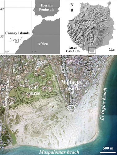
The dunes of Maspalomas cover an area of 403.9 ha and were declared a Special Natural Reserve by Law 12/1994, of 19 December, on Natural Spaces of the Canary Islands. This protected area is located at the southern part of the island of Gran Canaria (Spain), being one of the few dune ecosystems that still survives in the Canary Islands, but that is being degraded due to the high anthropogenic pressure related to tourism (Figure 1).

Figure 1. Location of special natural reserve of Dunas de Maspalomas.

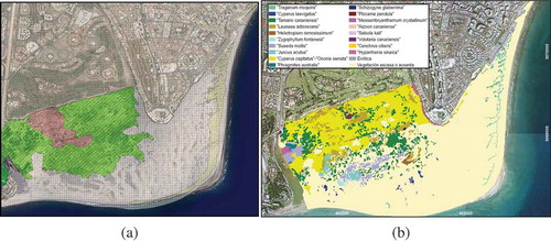
Plant communities in Maspalomas are subject to variability, and their presence and abundance may change due to dune dynamics, interannual variations of rainfall and the rate of reproduction and growth (Hernández Cordero, Pérez-Chacón, and Hernández-Calvento 2006; Hernández-Cordero, Hernández-Calvento, and Pérez-Chacón 2015b). These alterations, referring to plant communities, reveal changes and disturbances in the dune system of Maspalomas. Thus, it is crucial to have a detailed mapping of their distribution, as a basis for the proper management of this protected natural space. Cartography from local, regional or national administrations does not provide detailed information about the species distribution and the only cartography available of plant species was produced, as indicated, a decade ago in a research work using fieldwork and GIS techniques (Hernández Cordero, Pérez-Chacón, and Hernández-Calvento 2008; Hernández-Cordero, Pérez-Chacón, and Hernández-Calvento 2015a) (Figure 2).

Figure 2. Vegetation maps of Dunas de Maspalomas: (a) Canary Islands Government (map performed between 1999 and 2001, (Del Arco Aguilar 2009) and (b) Research work (Hernández Cordero, Pérez-Chacón, and Hernández-Calvento 2008).

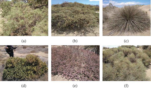
A total of 19 vegetal communities have been identified in the dunes field (Hernández-Cordero, Pérez-Chacón, and Hernández-Calvento 2015a), although only non-herbaceous species, as well as the most abundant and occupying a greater surface area will be analyzed in this work (Figure 3). Due to the arid climate of the study area, vegetation has a great seasonal and interannual variability depending on the rainfall distribution throughout the year and on the total accumulated annual amount. Rainfall produces a variation in the abundance of the plants according to the alternation between dry and wet years, as well as the contrast between the dry season (summer), when precipitation is absent, and the possible rainy season (autumn and winter) if the year is wet (Hernández Cordero, Pérez-Chacón, and Hernández-Calvento 2006). Likewise, the displacement of mobile dunes produces variations in the spatial distribution of plant species, as in short periods of time plants can disappear when buried by sand (Hernández-Cordero, Hernández-Calvento, and Pérez-Chacón 2015b).

Figure 3. Plant species of Maspalomas analyzed: (a) Tamarix canariensis, (b) Traganum moquinii, (c) Juncus acutus, (d) Tetraena fontanesii, (e) Suaeda mollis and (f) Launaea arborecens.

Satellite data

Very high resolution WorldView-2 (WV-2) satellite images obtained on 17 January 2013 and 4 June 2015 were used (Figure 4). In addition, a field campaign was performed, during 2015 and simultaneously to the satellite pass, to collect vegetation information.

Figure 4. Worldview-2 color composite images (Red: band 5, Green: band 3 and Blue: band 2) for the central area of the natural reserve of maspalomas: (a) 17 january 2013 and (b) 4 june 2015.

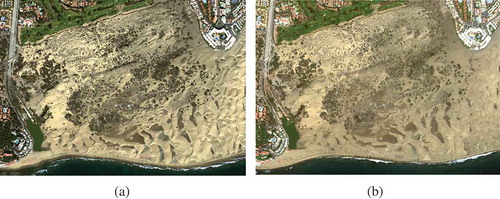
The WV-2 satellite carries two sensors capable of offering panchromatic (PAN) and multispectral (MS) imagery with resolutions of 0.46 m and 1.84 m, respectively. The MS image has 8 spectral bands that record the radiation in the following channels: coastal (400–450 nm), blue (450–510 nm), green (510–580 nm), yellow (585–625 nm), red (630–690 nm), red edge (705–745 nm), Near Infrared (NIR1) (770–895 nm), and NIR2 (860–1040 nm). Its nominal swath width is 16,4 km and the radiometric resolution is 11 bits (DigitalGlobe 2010). Table 1 illustrates the acquisition information of the satellite images used.

Table 1. Acquisition information of the WV-2 satellite images.

Date	17 January 2013	4 June 2015
Processing level	ORStandard2A	ORStandard2A
Mean Sun Azimuth	157,3º	103,9º
Mean Sun Elevation	38,4º	73,1º
Mean Sat Azimuth	101,2º	95,5º
Mean Sat Elevation	62,6º	81,1º
Mean Off-Nadir View Angle	24,2º	7,9º

Field measurement

Regarding the ground validation collection procedure for the characterization of the different plant species, an ASD FieldSpec-3 field spectroradiometer was used, which records the spectral radiance of the measured object and the radiance of the Spectralon@ reference panel. At each site, apart from the nadir, several radiance measurements were acquired at a typical height of 60 to 90 cm from the plant canopy and at different angles to obtain comparable measurements to the satellite and to better characterize the plant canopy and its spectral response (Jiménez et al. 2014). Measurements were recorded in the visible, near-infrared, and shortwave-infrared range of the spectrum (350–2500 nm) and over homogeneous and flat areas. In addition, precise geographic coordinates and time data were collected using a precise Global Positioning System (GPS) receiver, solar azimuth and zenithal angles were recorded and the ozone column, total water vapor and aerosol optical thickness was measured using the handheld sun-photometer. Figure 5 shows the locations of the sample points used in the classification procedure.

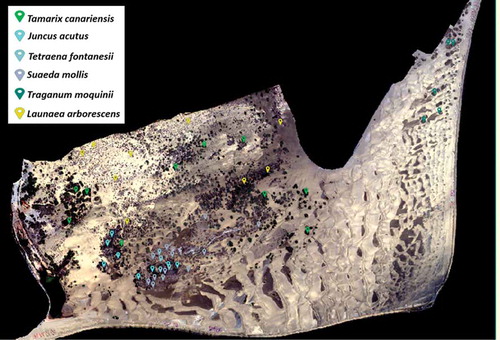
Figure 5. Locations of the sample points on a Worldview-2 color composite image of Maspalomas.

Atmospheric correction

There are different approaches to correct satellite data for atmospheric effects. Basically, techniques based on complex radiative models of the atmosphere and simpler methods exclusively relying on information from the image (Abdolrassoul and Turner 2007; Deidda and Sanna 2012; Martín et al. 2012; Marcello et al. 2016;). Two commonly used image-based atmospheric correction techniques are Dark Object Subtraction (DOS) (Chavez 1996) and QUick Atmospheric Correction (QUAC) (Bernstein et al. 2012). As indicated, more complex radiative methods model the atmosphere to remove the scattering and absorption atmospheric effects, such as MODTRAN (MODerate resolution atmospheric TRANsmission) (Adler-Golden et al. 1999), FLAASH (Fast Line-of-sight Atmospheric Analysis of Spectral Hypercubes) (Cooley et al. 2002), 6S (Second Simulation of a Satellite Signal in the Solar Spectrum) (Vermote et al. 2006) and ATCOR (ATmospheric CORrection) (Richter and Schläpfer 2005).

To perform the assessment of 5 representative algorithms (DOS, QUAC, FLAASH, 6S and ATCOR), satellite and ground-validation data were compared. 6S was implemented in C++, QUAC and FLAASH were evaluated using ENVI (ENVI 2004) and ATCOR was run in ERDAS (Erdas 2009). It is important to note that WV-2 measures the energy in channels of more than 40 nm of bandwidth and, thus, provides averaged reflectivities for all the bandwidth. However, the reflectivity of the field radiometer is measured in narrow bandwidths close to 1 nm. For this reason, the corrected reflectivity measurements of the WV-2 bands and the data recorded by the radiometer do not turn out to be quantitatively comparable. As a result, to obtain an analogous result for both instruments, the simulation of multispectral bands using the hyperspectral data provided by the field radiometer is used. This simulation consists of obtaining the integrated surface reflectivity band, ${\rho }_{\lambda ,integrated}^{radiometer}$, multiplying the normalized multispectral response function (NMRF) of the WV-2 bandpass filter of the band by the monochromatic reflectivity value of the field radiometer. In this way, an integration of the reflectivity of the radiometer for each WV-2 multispectral band from λ_min to λ_max is obtained by (Khandelwal and Rajan 2014) :

(1) ${\rho }_{\lambda ,integrated}^{radiometer}=\sum _{\lambda ={\lambda }_{min}}^{{\lambda }_{max}}{\rho }_{\lambda }^{radiometer}\ast NMR{F}_{\lambda }^{band}$(1)

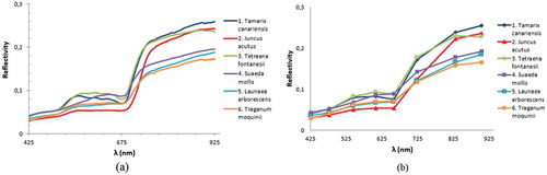
Figure 6. shows the mean reflectivity measures recorded by the ADS FieldSpec-3 the 4th of June 2015 for each plant species and the result after the integration using the spectral response function of the WV-2 satellite.

Figure 6. Spectral signatures of the vegetation species: (a) recorded by the field spectro-radiometer and (b) after the integration of the narrow bands to simulate the WV-2 bands.

Vegetation indices

Vegetation Indices (VIs) are based on the absorption and reflectance characteristics of plants in the visible and NIR regions. They have been widely used for predicting biophysical parameters of natural ecosystems. Specifically, VIs are mathematical combinations of different spectral bands that, basically, include ratios and linear combinations. A VI main advantage is that it enhances information contained in the spectral reflectance by detecting the spectral variability that might be due to different vegetation, plant, canopy or leaf physiological, and morphological characteristics (Omer et al. 2016). Moreover, VIs are efficient remotely sensed variables for reducing the noise due to, for example, atmospheric conditions, sun view angles, canopy geometry, shading, and soil background. In this study, 23 VIs (Table 2) were computed and tested in this specific ecosystem to improve the accuracy of the classification methodology.

Table 2. Spectral vegetation indices assessed to improve the classification performance.

Vegetation Index	Expression	Reference		Eq.
Simple Ratio Index (SRI)	$\frac{NIR1}{RED}$		(Jordan 1969)	(2)
Normalized Difference Vegetation Index (NDVI)	$\frac{NIR1-RED}{NIR1+RED}$		Rouse et al. 1973)	(3)
Transformed Vegetation Index (TVI)	$\sqrt{NDVI+0.5}$		(Deering and Rouse 1975)	(4)
Non-Linear Index (NLI):	$\frac{NIR{1}^2-RED}{NIR{1}^2+RED}$		(Goel and Qin 1994)	(5)
Atmospherically Resistant Vegetation Index (ARVI)	$\frac{NIR2-\left[\left(2.RED\right)-BLUE\right]}{NIR2+\left[\left(2.RED\right)-BLUE\right]}$		(Kaufman and Tanre 1992)	(6)
Structure-Insensitive Pigment Index (SIPI)	$\frac{NIR1-BLUE}{NIR1-REDEDGE}$		(Peluelas, Baret, and Filella 1995)	(7)
Renormalized Difference Index (RDI)	$\frac{NIR1-RED}{\sqrt{NIR1+RED}}$		(Roujean and Breon 1995)	(8)
Green Normalized Difference Vegetation Index (GNDVI)	$\frac{NIR1-GREEN}{NIR1+GREEN}$		Gitelson and Merzlyak M.N 1996)	(9)
Modified Simple Ratio MSR (MSR)	$\frac{\frac{NIR1}{RED}-1}{\sqrt{\frac{NIR1}{RED}+1}}$		(Chen 1996)	(10)
Pigment Specific Simple Ratio (Chlorophyll a) (PSSRa)	$\frac{NIR1}{REDEDGE}$		(Blackburn 1998)	(11)
Plant Senescence Reflectance Index (PSRI)	$\frac{REDEDGE-BLUE}{NIR1}$		(Merzlyak et al. 1999)	(12)
Enhanced Vegetation Index (EVI)	$2.5\frac{\left(NIR1-RED\right)}{NIR1+6RED-7.5BLUE+1}$		(Huete, Justice, and Van Leeuwen 1999)	(13)
Modified Chlorophyll Absorption in Reflectance Index (MCARI)	$\left[\left(REDEDGE-RED\right)-0.2\left(REDEDGE-GREEN\right)\right]\frac{REDEDGE}{RED}$		(Daughtry et al. 2000)	(14)
Modified Simple Ratio (MSR)	$\frac{NIR1-BLUE}{RED-BLUE}$		(Sims and Gamon 2002)	(15)
Difference Vegetation Index (DVI)	$NIR1-RED$		(Richardson and Wiegand 1977)	(16)
Transformed Chlorophyll Absorption in Reflectance Index (TCARI)	$3\left[\left(REDEDGE-RED\right)-0.2\left(REDEDGE-GREEN\right)\left(\frac{REDEDGE}{RED}\right)\right]$		(Haboudane et al. 2002)	(17)
Visible Atmospherically Resistant Index (VARI)	$\frac{GREEN-RED}{GREEN+RED-BLUE}$		(Gitelson et al. 2002)	(18)
Visible Green Index (VGI)	$\frac{GREEN-RED}{GREEN+RED}$		(Gitelson et al. 2002)	(19)
Modified Normalized Difference (MND)	$\frac{NIR1-BLUE}{NIR1+REDEDGE-2BLUE}$		(Sims and Gamon 2002)	(20)
Carotenoid Reflectance Index (CRI)	$\frac{1}{BLUE}-\frac{1}{REDEDGE}$		(Gitelson et al. 2002)	(21)
Green Index (GI):	$\frac{NIR1}{GREEN}-1$		(Gitelson et al. 2005)	(22)
Red Index (RI)	$\frac{NIR1}{RED}-1$		(Gitelson et al. 2005)	(23)
Modified Soil Adjusted Vegetation Index 2 (MSAVI2)	$\frac{\left(2\ast NIR1+1-\sqrt{{\left(2\ast NIR1+1\right)}^2-8\ast \left(NIR1-RED\right)}\right)}{2}$		(Qi et al. 1994)	(24)

Textural information

Another source of ancillary data is the spatial distribution of gray tones in the image (texture). The benefits of incorporating texture in land cover classification have been pointed out in numerous studies making use of different classification algorithms and texture measures (Anys et al. 1994; Puissant, Hirsch, and Weber 2005; Mather and Tso 2016, Ibarrola-Ulzurrun, Gonzalo-Martín, and Marcello 2017b). Texture contains important information about the structural arrangement of surfaces and their relationship to the surrounding environment. An approach which yields good results consists of extracting different parameters by means of the Gray-Level Co-occurrence Matrix (GLCM) method (Haralick and Shanmugam 1973), and using such textural information as additional bands in the classification process. To avoid redundancy, the Principal Component Analysis (PCA) was first applied to the multispectral image to get a new set of components ordered in decreasing significance of variance and, then, the GLCM is was computed on the first principal component (Hall-Beyer 2017). After analyzing different textural parameters, four textural maps (variance, homogeneity, dissimilarity and entropy) were explored as additional information sources to improve the accuracy of the classification (Li et al., 2014).

Unmixing

Due to limitations in the spatial resolution of satellite sensors and the reduced size of the plant species analyzed, certain pixels of the image may represent a mixture of spectral signatures of different coverages (i.e. vegetation and soil or mixture of different plant species). Therefore, unmixing consists of estimating the contribution percentage (abundance) of each pure class (endmember) to the total reflectivity of the pixel. Linear mixing models provide acceptable results in a large number of applications (Heinz 2001; Bioucas et al. 2012) and although a non-linear model can be more precise when dealing with high spatial resolution imagery, its application requires prior and detailed information about the geometry and physical properties of the objects, which hinders its usefulness.

There are different strategies for the selection of endmembers. In this work, after testing different approaches, the spectral signatures measured for each species in the field campaign, simultaneously to the satellite pass, were used. They represent the endmembers used as references for the linear unmixing process (Jiménez, Pou, and Díaz-Delgado 2011; Díaz Delgado, Lucas, and Hurford 2017).

Classification methodology

Classification involves different steps. The first step was to determine the classes to be discriminated. As indicated, the vegetation classes chosen for this ecosystem were selected by experts of the Special Natural Reserve of Dunas de Maspalomas, being: Traganum moquinii, Suaeda mollis, Launaea arborecens, Tetraena fontanesii, Tamarix canariensis and Juncus acutus. The next step in a supervised classification consists of labelling a sufficient number of regions of interest (ROIs). The selected pixels were divided into two groups (pixels for calibration and validation of the classifiers) so as to remove any possible bias that could be caused by using the same dataset (Myburgh 2012). More than 5 ROIs for each species were selected to account for the variability of each class. In total, the minimum number of pixels considered for each class was 40 × number of wavebands which, in most cases, give satisfactory results. The method used for choosing the samples was a random method in which a 70% of the total samples were chosen as calibration samples and 30% of the total samples for the validation. Before performing the classification process, the Jeffries-Matusita distance (Mather and Tso 2016) was computed in order to check the separability of each vegetation class. This distance ranges from 0 to 2, being 2 a perfect separability value between classes.

As suggested in preliminary studies (Pal and Mather 2005; Mountrakis, Im, and Ogole 2011; Mather and Tso 2016; Maulik and Chakraborty 2017), SVM was selected as the appropriate classification algorithm (Cortes and Vapnik 1995; Vapnik and Vapnik 1998, 1999; Weston et al. 1999, 2001), because, in general, SVM is more robust for the size and quality of the calibration dataset (Mountrakis, Im, and Ogole 2011; Zhao et al. 2016). Nowadays, deep learning approaches (Yu et al. 2017) are becoming popular; however, they require a large calibration dataset, and thus are an inconvenience for many operational applications. Also, a recent assessment comparing advanced classification methods (SVMs, RFs, neural networks, deep CNNs, logistic regression-based techniques, and sparse representation-based classifiers) demonstrates that SVM is widely used because of its accuracy, stability, automation and simplicity (Ghamisi et al. 2017).

SVM is based on statistical learning theory which aims to determine the location of decision boundaries that produce the optimal separation of classes and does not require assumption on their distribution. The concept of the kernel was introduced to extend the capability of the SVM to deal with nonlinear decision surfaces. To select the kernel and its parameters, a grid search strategy was applied using the classification accuracy as the measure of quality (Kavzoglu and Colkesen 2009). The kernel selected was the Radial Basis Function (Yang 2011; Dixit and Agarwal 2013; Lin and Yan 2016) due to its superior performance, in general, and the two parameters to be optimized were C and ɣ, where C is a penalty parameter that controls the trade off between errors of the SVM on calibration data and margin maximization and ɣ is the width of the Radial Basis Function.

To select the best mapping methodology, different schemes were considered injecting, to the SVM classifier, spectral and spatial information extracted from the multispectral image. The combinations analyzed were:

• Bands (multispectral bands after the corrections).

• Vegetation indices (complete set of VIs).

• Bands and vegetation indices (best VIs).

• Bands and texture.

• Bands and vegetation indices and texture.

• Abundance of each class after the linear unmixing processing.

The vegetation and texture maps were generated with C++ routines, as well the abundance maps from the linear unmixing model. The SVM classification was configured and evaluated using the ENVI software.

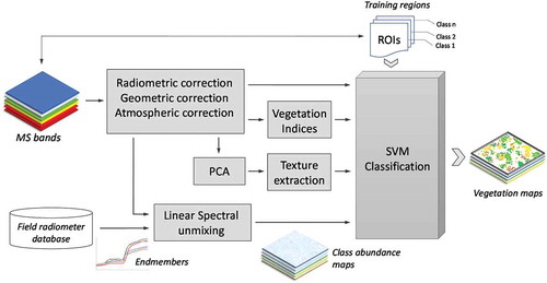
Figure 7 shows the overall schematics of the different strategies assessed. Image corrections are the first steps to apply. Radiometric correction refers to pixel conversion from digital level to radiance, while the atmospheric correction estimates the Top of Canopy (TOC) reflectance. Geometric correction is usually performed by the provider but the images were orthorectified to remove terrain distortions. Vegetation maps were obtained by applying classification techniques to the different feature combinations using the same calibration samples.

Figure 7. General classification scheme with the different input combinations (multispectral bands, vegetation indices, texture measures and abundances after the linear unmixing) to the SVM algorithm.

The accuracy of the classification was measured by using the validation samples collected and the information provided by the expert. The statistical accuracy assessment considered in the study was the standardized Confusion Matrix, which reports 2 global measurements of accuracy: Overall Accuracy and Kappa coefficient (Congalton 1991).

To assess the remote sensing classification, comparison with the existing GIS and field work vegetation cartography (Hernández Cordero, Pérez-Chacón, and Hernández-Calvento 2008; Hernández-Cordero, Pérez-Chacón, and Hernández-Calvento 2015a) was not performed because the former represents plant species while the latter refers to plant communities. In addition, a significant period of time of over 10 years has passed between both maps and the area of mobile dunes has changed considerably. Also, in the stabilized dunes there have been changes in the vegetation due to processes of ecological succession. For this reason, the results obtained by remote sensing were additionally validated through photointerpretation of the WV-2 satellite image and the digital orthophoto (spatial resolution of 25 cm/pixel) from 2015. Specifically, a systematic sampling was carried out to generate a grid of points every 50 meters in the GIS, obtaining a total of 1427 points. Of these, the 290 points matching with plants were selected, where 93 correspond to Launaea arborescens, 78 to Tamarix canariensis, 57 to Suaeda mollis, 39 to Traganum moquinii, 16 to Tetraena fontanesii and 7 to Juncus acutus. In each of these points, an expert compared the remote sensing classification with the ground-validation, obtaining the accuracy percentage.

Results and discussion

Remote sensing image corrections

The aim of the image corrections study was to assess the accuracy of different atmospheric corrections methodologies. As indicated, co-temporal in-situ and satellite data were available for June 4th, 2015. This work compared 5 atmospheric correction algorithms (3 model-based and 2 image-based) applied to the 8 bands of the WV-2 satellite. The study consisted of comparing, for each vegetation species, the estimated TOC reflectivity from the WV-2 corrected images with respect to the in-situ reflectance measures, after the mentioned integration of narrow bands. For this comparative analysis, graphical representation and a statistical assessment (RMSE and BIAS) were carried out.

Regarding the atmospheric models FLAASH, 6S and ATCOR, different parameters were specified. The Mid-Latitude Summer atmosphere type is the most appropriate for Canary Islands climate. The most suitable aerosol model for the islands is the maritime model. The AOT value has to be carefully selected, using direct measurements or satellite estimates, because it has a major effect in the surface reflectance calculated. In this analysis, the real data measured during the field campaign was used. As indicated, the appropriate parameter configuration is key to carrying out a precise atmospheric correction in many applications (Marcello et al. 2016).

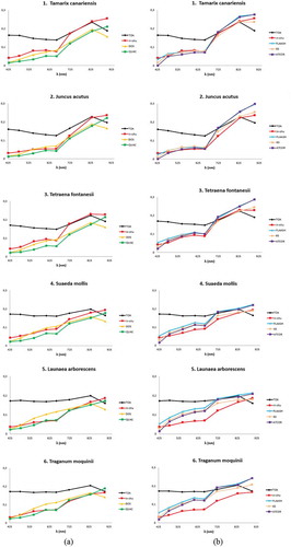
Figure 8 shows the spectral signatures of the vegetation sites selected during the field campaign. The reflectance estimated for each Worldview-2 band and the real value measured at ground level are included. For WV-2, the reflectivity corrected by each image-based (left) and model-based (right) algorithm, as well as the Top of Atmosphere (TOA) reflectance without any correction, are shown. One can see that, in general, algorithms based on radiative modeling perform better, with their spectral signature resembling those obtained with the in-situ measurements. In particular, 6S seems to be more accurate than FLAASH and ATCOR. Image-based algorithms tend to underestimate the values of reflectivity for most plant species. In addition, the DOS method degrades the typical spectral signature of vegetation. On the other hand, model-based algorithms tend to slightly overestimate the real reflectivities but properly match the spectral signature of vegetation.

Figure 8. Spectral signatures of each vegetation species comparing in-situ data and atmospheric correction algorithms: (a) image-based and (b) model-based.

The average results for all the vegetation points analyzed are included in Tables 3 and 4, where the RMSE and BIAS between measured and satellite corrected reflectance are presented. Results demonstrate that atmospheric correction applying algorithms based on the physical modelling are more precise. They obtain good estimations with, in general, low RMSE values and negligible BIAS when compared with field data. Results corroborate that 6S is the most accurate when estimating the vegetation points real spectral signatures (Mean RMSE of 0,8%). In some cases, DOS and QUAC show acceptable numerical results that are unrealistic because the RMSE and BIAS values presented are average values for the 8 bands and some values can compensate others.

Table 3. RMSE between measured reflectivity values and corrected atmospherically in the WV-2 image of 2015 for all the vegetation points.

	DOS	QUAC	FLAASH	6S	ATCOR
Tamarix canariensis	0,0154	0,0142	0,0049	0,0047	0,0071
Juncus acutus	0,0106	0,0077	0,0105	0,0055	0,0112
Tetraena fontanesii	0,0128	0,0137	0,0089	0,0043	0,0088
Suaeda mollis	0,0090	0,0082	0,0108	0,0066	0,0088
Launaea arborescens	0,0108	0,0039	0,0176	0,0124	0,0135
Traganum moquinii	0,0078	0,0043	0,0202	0,0143	0,0180
MEAN RMSE	0,0111	0,0087	0,0122	0,0080	0,0112

Table 4. BIAS between measured reflectivity values and corrected atmospherically in the WV-2 image of 2015 for all the vegetation points.

	DOS	QUAC	FLAASH	6S	ATCOR
Tamarix canariensis	−0,0317	−0,0386	0,0063	−0,0081	−0,0034
Juncus acutus	−0,0145	−0,0192	0,0212	0,0089	0,0143
Tetraena fontanesii	−0,0145	−0,0192	0,0212	0,0089	0,0143
Suaeda mollis	−0,0121	−0,0230	0,0292	0,0118	0,0167
Launaea arborescens	0,0049	−0,0075	0,0468	0,0266	0,0303
Traganum moquinii	0,0101	−0,0015	0,0548	0,0371	0,0434
MEAN BIAS	−0,0096	−0,0182	0,0299	0,0142	0,0193

Classification

Once the WV-2 image of 2015 was properly corrected using the 6S model, the classification methodology was applied. The following results present the accuracy of the SVM classification method applying the different input combinations detailed in Figure 7.

After the spectral separability analysis (Table 5), it was observed that some pair of classes have low separability values (Jeffries-Matusita distance around 1.4). This is the case of Tetraena fontanesii, which will be more difficult to discriminate due to its spectral similarity with Suaeda mollis and Launaea arborescens. On the other hand, Tamarix canariensis is the most separable species with distance values between 1,7 and 1,9 for Juncus acutus and Traganum moquinii respectively.

Table 5. Spectral separability analysis for the training samples.

	Tamarix canariensis	Tetraena fontanesii	Traganum moquini	Suaeda mollis	Juncus acutus
Tamarix canariensis
Tetraena fontanesii	1,959
Traganum moquini	1,955	1,544
Suaeda mollis	1,978	1,428	1,776
Juncus acutus	1,733	1,948	1,994	1,974
Launaea arborescens	1,937	1,428	1,633	1,369	1,901

Table 6 shows a summary of the overall accuracy, as well as the Kappa coefficient, for the best classification methodologies assessed. Support Vector Machine with MSAVI2 plus the variance texture map reaches the highest Overall Accuracy (88,03%). It shows how the MSAVI2 index improves the precision compared with the MS bands. Also, the variance texture map improves the results; highlighting the importance of including spatial information in the classifier. Despite having only information in 8 bands, the results obtained with linear unmixing techniques are acceptable and allow proper discrimination of certain plant species.

Table 6. Overall accuracy and kappa coefficient for the support vector machine classifier with different input band combinations.

	Overall accuracy		Kappa
Bands		86,40%	0,817
Vegetation indices		86,34%	0,815
Bands + MSAVI2		87,12%	0,826
Bands + Texture		87,17%	0,826
Bands+ MSAVI2+ Texture		88,03%	0,838
Unmixing abundances		81,46%	0,717

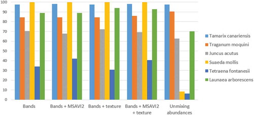
In more detail, and to identify the vegetation discrimination capability of vegetation species, Figure 9 shows the overall accuracy percentage for each class and methodology. In general, the percentages of success are high for most species except for Tetraena fontanesii, which shows lower percentages, as expected because of its low separability values with the rest of species. In any case, it highlights the fact that inclusion of the MSAVI2 vegetation index improves its accuracy with an overall accuracy increase from 34,15% to 42,11%. On the other hand, introducing additional information, such as the texture variance map, helps to discriminate Launaea arborescens, whose accuracies increase to 94,03% compared to the other methodologies tested (88,89% including bands+MSAVI2). Finally, including the spectral and spatial information balances the percentages of success of these two critical species.

Figure 9. Overall accuracy of each vegetation species and input combination.

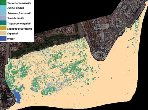
Figure 10 includes the thematic map generated with the methodology achieving the best performance. The visual interpretation indicates that most of the pixels are classified in accordance with the reference cartographic map of the Figure 2(b) and match the expert´s knowledge of plant distribution and the field campaign. As detected in Figure 9, some species like Tetraena fontanesii are misclassified because they are small and are mixed with other species.

Figure 10. Vegetation map of the special natural reserve of Dunas de Maspalomas using the Worldview-2 image of 4 june 2015.

On the other hand, validation by photointerpretation highlights that 3 plant species achieve a significant percentage of well-classified points, specifically Tamarix canariensis (94,9%), Juncus acutus (85,7%) and Launaea arborescens (62,4%). In contrast, Traganum moquinii, Suaeda mollis and Tetraena fontanesii get much lower accuracies. In any case, the spatial analysis in the GIS identified well classified areas that were not sampled because these species are densely concentrated together and the sampling performed did not get the suitable number of samples. The poor classification of the three indicated plant species can be due to several reasons. On one hand, the morphological characteristics of the plants, such as Suaeda mollis and Tetraena fontanesii, which are low and small in diameter, usually lower than the spatial resolution of the satellite image. Therefore, to be properly classified they must have higher size and density that encompasses the entire pixel. Another factor could be related to these species low density foliage which causes them to be confused with the substrate where they grow. This fact is especially relevant under the conditions of the arid climate of Maspalomas, since dry years or pronounced seasonality of precipitations produce a great hydric stress on the plants that hinder the development of a significant biomass. Finally, the some plant species similar spectral signature produces confusion among some of them.

As indicated, MSAVI2 was selected as the most suitable vegetation index to discriminate between plant species. To identify the best VI, an exhaustive analysis of the accuracy of the SVM classifier was carried out adding to the WV-2 bands each spectral index independently. The graph of Figure 11 shows the results obtained for the 23 vegetation indices detailed in Table 2. It identifies MSAVI2 as offering the highest overall accuracy, with slightly better values than TVI and NLI. Thus, MSAVI2 was selected for the final classification methodology, confirming its good performance in arid ecosystems. Additional combinations, adding 2 and 3 of the best indices to the spectral bands, were also tested but the accuracy did not improve.

The arid climate of the dunes of Maspalomas makes it difficult to analyze the abundance and spatial distribution of the plant communities, since in dry years and seasons (summer) the annual species do not grow and some shrub species lose part of their leaves, which makes their detection by remote sensing difficult. In addition, one of the limitations of the proposed method is that it does not detect small herbaceous plant communities such as those formed by Cyperus capitatus and Ononis tournefortii, classified as dry sand. In any case, the results for the June image corroborate the methodology´s good performance. Moreover, the best processing protocol was also applied to the winter image of January 2013 providing excellent results as well (Figure 12).

Figure 11. Overall accuracy of the 23 vegetation indices tested (Accuracy for the WV-2 bands is also included as a reference).

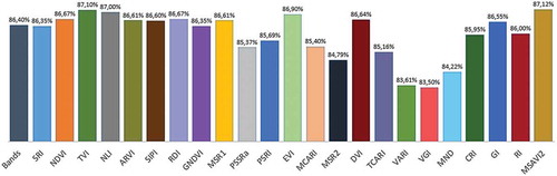
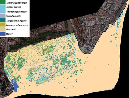
Figure 12. Vegetation map of the special natural reserve of Dunas de Maspalomas using the Worldview-2 image of 17 january 2013.

Conclusions

In this work, a processing methodology for the mapping of plant species has been developed for Maspalomas dunes, based on the use of advanced satellite imagery and the analysis of different processing techniques is fundamental to obtain accurate and reliable results. This satellite derived cartography provides a systematic and fast procedure to monitor the dune ecosystem status and to process the limited information available to the conservation managers. This is due to the fact that current vegetation maps, available from regional or national administrations, do not provide detailed information about species distribution and the only cartography available of plant species was performed manually in 2003.

Atmospheric correction is important for the physical interpretation of remote sensing data and to precisely derive spectral indices. However, due to its complexity and the lack of a method demonstrating superior performance, an assessment of different algorithms and configurations was conducted to accurately estimate the reflectivity of the selected plant species. 6S achieved the lowest RMSE and, as a result, was the selected algorithm.

To develop a classification methodology, different strategies were evaluated, including additional spectral and spatial information to the multispectral WV-2 bands and the application of unmixing techniques to get the abundance maps of each species.

After the analysis performed, it was concluded that the methodology achieving the best performance (overall accuracy of 88,03%) is based on the SVM classifier with the corrected multispectral bands plus a vegetation index (MSAVI2) and a band of contextual information (variance). It was demonstrated that abundance maps, obtained with linear unmixing techniques using the pure spectral signatures from field radiometer data, offer acceptable results but of lower accuracy. This was probably due to the limited number of bands in the WV-2 image and the similar spectral behavior of certain plant species.

The proposed classification methodology has been applied on WV-2 images belonging to different seasons of the year. Results have demonstrated the robustness to changes related to the phenological state of the vegetation, which is essential in an arid environment such as the dunes of Maspalomas, where seasonal and interannual changes of plant communities can be very significant due to the variable rainfall. Finally, photointerpretation comparison using a digital orthophoto from 2015 has provided satisfactory results for Tamarix canariensis, Juncus acutus and Launaea arborescens while for other species with lower density and size it was less accurate.

Due to the complexity of the ecosystem and the spectral similarity of the species, a hyperspectral aircraft flight campaign was recently performed and another one using a drone is planned to check the ability of hyperspectral imagery to improve the discrimination capability of some species.

Acknowledgements

This work has been supported by the ARTEMISAT (CGL2013-46674-R) and ARTEMISAT-2 (CTM2016-77733-R) projects, funded by the Spanish Agencia Estatal de Investigación (AEI) and the European Fondo Europeo de Desarrollo Regional (FEDER).

Disclosure statement

No potential conflict of interest was reported by the authors.

Additional information

Funding

This work was supported by the Agencia Estatal de Investigación | Ministerio de Economía y Competitividad (CTM2016-77733-R) (CGL2013-46674-R)

References

- Abdolrassoul, S. M., and B. J. Turner. 2007. “A Comparison of Four Common Atmospheric Correction Methods.” Photogrammetric Engineering & Remote Sensing 73 (4): 361–368. doi:10.14358/PERS.73.4.361.
- Adler-Golden, S. M., M. W. Matthew, L. S. Bernstein, R. Y. Levine, A. Berk, S. C. Richtsmeier, P. K. Acharya, et al. 1999. “Atmospheric Correction for Short-Wave Spectral Imagery Based on MODTRAN4.” In Imaging Spectrometry V. International Society for Optics and Photonics 3753 :61–70. doi:10.1117/12.366315.
- Anys, H., A. Bannari, D. C. He, and D. Morin. 1994. “Texture Analysis for the Mapping of Urban Areas Using Airborne MEIS-II Images.” First International Airborne Remote Sensing Conference and Exhibition. Environmental Research Institute of Michigan 3: 231–245.
- Bernstein, L. S., S. M. Adler-Golden, X. Jin, B. Gregor, and R. L. Sundberg. 2012. “Quick Atmospheric Correction (QUAC) Code for VNIR-SWIR Spectral Imagery: Algorithm Details.“. IEEE Workshop on Hyperspectral Image and Signal Processing, Shagai, China. doi:10.1109/WHISPERS.2012.6874311.
- Bioucas, J., A. Plaza, N. Dobigeon, M. Parente, Q. Du, P. Gader, and J. Chanussot. 2012. “Hyperspectral Unmixing Overview: Geometrical, Statistical, and Sparse Regression-Based Approaches.” IEEE Journal of Selected Topics in Applied Earth Observation and Remote Sensing 5 (2): 354–379. doi:10.1109/JSTARS.2012.2194696.
- Blackburn, G. A. 1998. “Spectral Indices for Estimating Photosynthetic Pigment Concentrations: A Test Using Senescent Tree Leaves.” International Journal of Remote Sensing 19: 657–675. doi:10.1080/014311698215919.
- Cabrera Vega, L. L., N. Cruz-Avero, L. Hernández-Calvento, A. I. Hernández-Cordero, and E. Fernández Cabrera. 2013. “Morphological Changes in Dunes as an Indicator of Anthropogenic Interferences in Arid Dune Fields.” Journal of Coastal Research 65: 1271–1276. doi:10.2112/SI65-215.1.
- Chavez, P. S. 1996. “Image-Based Atmospheric Corrections-Revisited and Improved.” Photogrammetric Engineering and Remote Sensing 62 (9): 1025–1035.
- Chen, J. M. 1996. “Evaluation of Vegetation Indices and a Modified Simple Ratio for Boreal Applications.” Canadian Journal of Remote Sensing 22: 229–242. doi:10.1080/07038992.1996.10855178.
- Congalton, R. G. 1991. “A Review of Assessing the Accuracy of Classifications of Remotely Sensed Data.” Remote Sensing of Environment 37 (1): 35–46. doi:10.1016/0034-4257(91)90048-B.
- Cooley, T., G. P. Anderson, G. W. Felde, M. L. Hoke, A. J. Ratkowski, J. H. Chetwynd, J. A. Gardner, et al. 2002. “FLAASH, a MODTRAN4-based Atmospheric Correction Algorithm. Its Application and Validation.” IEEE International Geosciences and Remote Sensing Symposium 3: 1414–1418. doi:10.1109/IGARSS.2002.1026134.
- Cortes, C., and V. Vapnik. 1995. “Support-Vector Networks.” Machine Learning 20: 273–297. doi:10.1023/A:1022627411411.
- Daughtry, C., C. Walthall, M. Kim, E. B. Colstoun, and J. McMurtrey. 2000. “Estimating Corn Leaf Chlorophyll Concentration from Leaf and Canopy Reflectance.” Remote Sensing of Environment 74: 229–239. doi:10.1016/S0034-4257(00)00113-9.
- Deering, D., and J. Rouse. 1975. “Measuring “Forage Production” of Grazing Units from Landsat MSS Data.” Proceedings of the 10th Intenational Symposium on Remote Sensing of Environment, Ann Arbor, MI, USA, 6–10.
- Deidda, M., and G. Sanna. 2012. “Pre-Processing of High Resolution Satellite Images for Sea Bottom Classification.” Italian Journal of Remote Sensing 44 (1): 83–95. doi:10.5721/ItJRS20124417.
- Del Arco Aguilar, M. J. 2009. Mapa De Vegetación De Canarias. Spain: GRAFCAN. Santa Cruz de Tenerife.
- Díaz Delgado, R., R. Lucas, and C. Hurford. 2017. The Roles of Remote Sensing in Nature Conservation: A Practical Guide and Case Studies. Switzerland: Springer.
- DigitalGlobe. 2010. “Radiometric Use of Worldview2 Imagery.” Revision 1.0: 1–10.
- Dixit, A., and S. Agarwal. 2013. “Comparison of Various Models and Optimum Range of Its Parameters Used in SVM Classification of Digital Satellite Image.” IEEE International Conference Image Information Processing 363–368. doi:10.1109/ICIIP.2013.6707616.
- ENVI. 2004. ENVI User’s Guide. Boulder. CO: Research Systems.
- Erdas, G. 2009. “ATCOR for ERDAS Imagine 2011–Haze Reduction, Atmospheric and Topographic Correction–User Manual ATCOR 2 and ATCOR 3.” ERDAS Imagine 1: 58.
- Ghamisi, P., J. Plaza, Y. Chen, J. Li, and A. Plaza. 2017. “Advanced Spectral Classifiers for Hyperspectral Images.” IEEE Geosciences and Remote Sensing Magazine 5 (1): 8–32. doi:10.1109/MGRS.2016.2616418.
- Gitelson, A. A., A. Vina, V. Ciganda, D. C. Rundquist, and T. J. Arkebauer. 2005. “Remote Estimation of Canopy Chlorophyll Content in Crops.” Geophysical Research Letters 32. doi:10.1029/2005GL022688.
- Gitelson, A. A., and M. N. Merzlyak M.N. 1996. “Signature Analysis of Leaf Reflectance Spectra: Algorithm Development for Remote Sensing of Chlorophyll.” Journal of Plant Physiology 148: 494–500. doi:10.1016/S0176-1617(96)80284-7.
- Gitelson, A. A., Y. J. Kaufman, R. Stark, and D. Rundquist. 2002. “Novel Algorithms for Remote Estimation of Vegetation Fraction.” Remote Sensing of Environment 80 (1): 76–87. doi:10.1016/S0034-4257(01)00289-9.
- Goel, N. S., and W. Qin. 1994. ”Influences of Canopy Architecture on Relationships between Various Vegetation Indices and LAI and fPAR: A Computer Simulation.”. Remote Sensing Reviews 10 (4): 309–347. doi:10.1080/02757259409532252.
- Haboudane, D., J. R. Miller, N. Tremblay, P. J. Zarco-Tejada, and L. Dextraze. 2002. “Integrated Narrow-Band Vegetation Indices for Prediction of Crop Chlorophyll Content for Application to Precision Agriculture.” Remote Sensing of Environment 81 (2): 416–426. doi:10.1016/S0034-4257(02)00018-4.
- Hall-Beyer, M. 2017. “Practical Guidelines for Choosing GLCM Textures to Use in Landscape Classification Tasks over a Range of Moderate Spatial Scales.” International Journal of Remote Sensing 38 (5): 1312–1338. doi:10.1080/01431161.2016.1278314.
- Haralick, R. M., and K. Shanmugam. 1973. “Textural Features for Image Classification.” IEEE Transactions on Systems, Man and Cybernetics 3 (6): 610–621. doi:10.1109/TSMC.1973.4309314.
- Heinz, D. C. 2001. “Fully Constrained Least Squares Linear Spectral Mixture Analysis Method for Material Quantification in Hyperspectral Imagery.” IEEE Transactions on Geoscience and Remote Sensing 39 (3): 529–545. doi:10.1109/36.911111.
- Hernández Calvento, L. 2006. Diagnóstico Sobre La Evolución Del Sistema De Dunas De Maspalomas (1960-2000). Spain: Cabildo de Gran Canaria, Las Palmas de Gran Canaria.
- Hernández Cordero, A. I., E. Pérez-Chacón, and L. Hernández-Calvento. 2006. “Vegetation Colonisation Processes Related to a Reduction in Sediment Supply to the Coastal Dune Field of Maspalomas (Gran Canaria, Canary Islands, Spain).” Journal of Coastal Research 48: 69–76.
- Hernández Cordero, A. I., E. Pérez-Chacón, and L. Hernández-Calvento. 2008. “Aplicación De Tecnologías De La Información Geográfica Al Estudio De La Vegetación En Sistemas De Dunas Litorales. Resultados Preliminares En El Campo De Dunas De Maspalomas.” XIII Congreso de Tecnologías de la Información Geográfica para el Desarrollo Territorial. Las Palmas de Gran Canaria, Spain.
- Hernández- Cordero, A. I., L. Hernández-Calvento, and E. Pérez-Chacón. 2017. “Vegetation Changes as an Indicator of Impact from Tourist Development in an Arid Transgressive Coastal Dune Field.” Land Use Policy 64: 479–491. doi:10.1016/j.landusepol.2017.03.026.
- Hernández-Calvento, L., D. W. T. Jackson, R. Medina, A. I. Hernández-Cordero, N. Cruz, and S. Requejo. 2014. “Downwind Effects on an Arid Dunefield from an Evolving Urbanised Area.” Aeolian Research 15: 301–309. doi:10.1016/j.aeolia.2014.06.007.
- Hernández-Cordero, A. I., E. Pérez-Chacón, and L. Hernández-Calvento. 2015a. “Vegetation, Distance to the Coast, and Aeolian Geomorphic Processes and Landforms in a Transgressive Arid Coastal Dune System.” Physical Geography 36 (1): 60–83. doi:10.1080/02723646.2014.979097.
- Hernández-Cordero, A. I., L. Hernández-Calvento, and E. Pérez-Chacón. 2015b. “Relationship between Vegetation Dynamics and Dune Mobility in an Arid Transgressive Coastal System, Maspalomas, Canary Islands.” Geomorphology 238: 160–176. doi:10.1016/j.geomorph.2015.03.012.
- Huete, A., C. Justice, and W. Van Leeuwen. 1999. MODIS Vegetation Index (MOD13). Algorithm Theoretical Basis Document. VA, USA: University of Virginia: Charlottesville.
- Ibarrola-Ulzurrun, E., C. Gonzalo-Martín, and J. Marcello. 2017a. “Influence of Pansharpening in Obtaining Accurate Vegetation Maps.” Canadian Journal of Remote Sensing 43 (6): 528–544. doi:10.1080/07038992.2017.1371583.
- Ibarrola-Ulzurrun, E., C. Gonzalo-Martín, and J. Marcello. 2017b. “Vulnerable Land Ecosystems Classification Using Spatial Context and Spectral Indices.” Proceedings SPIE Vol. 10428, Earth Resources and Environmental Remote Sensing/GIS Applications VIII. doi:10.1117/12.2278496.
- Isbell, F., V. Calcagno, A. Hector. 2011. “High Plant Diversity Is Needed to Maintain Ecosystem Services.” Nature 477 (7363): 199–202. doi:10.1038/nature10282.
- Jiménez, M., A. Pou, and R. Díaz-Delgado. 2011. “Cartografía De Especies De Matorral De La Reserva Biológica De Doñana Mediante El Sistema Hiperespacial Aeroportado INTA-AHS. Implicaciones En El Estudio Y Segimiento Del Matorral De Doñana.”. Revista De Teledetección 36: 98–102.
- Jiménez, M., M. González, A. Amaro, and A. Fernández. 2014. “Field Spectroscopy Metadata System Based on ISO and OGC Standards.” ISPRS International Journal of Geo-Information 3 (3): 1003–1022. doi:10.3390/ijgi3031003.
- Jordan, C. F. 1969. “Derivation of Leaf-Area Index from Quality of Light on the Forest Floor.” Ecology 50: 663–666. doi:10.2307/1936256.
- Kaufman, Y. J., and D. Tanre. 1992. “Atmospherically Resistant Vegetation Index (ARVI) for EOS-MODIS.” IEEE Transactions on Geosciences and Remote Sensing 30 (2): 261–270. doi:10.1109/36.134076.
- Kavzoglu, T., and I. Colkesen. 2009. “A Kernel Functions Analysis for Support Vector Machines for Land Cover Classification.” International Journal of Applied Earth Observation and Geoinformation 11 (5): 352–359. doi:10.1016/j.jag.2009.06.002.
- Khandelwal, A., and K. S. Rajan. 2014. “Sensor Simulation Based Hyperspectral Image Enhancement with Minimal Spectral Distortion.” ISPRS Annals of the Photogrammetry, Remote Sensing and Spatial Information Sciences 2 (8): 179. doi:10.5194/isprsannals-II-8-179-2014.
- Khare, S., and S. Ghosh. 2016. “Satellite Remote Sensing Technologies for Biodiversity Monitoring and Its Conservation.” International Journal of Advanced Earth Science and Engineering 5 (1): 375–389. doi:10.23953/cloud.ijaese.213.
- Li, M., S. Zhang, B. Zhang, S. Li, and C. Wu. 2014. “A Review of Remote Sensing Image Classification Techniques: The Role of Spatio-Contextual Information.” European Journal of Remote Sensing 47 (1): 389–411. doi:10.5721/EuJRS20144723.
- Lin, Z., and L. Yan. 2016. “A Support Vector Machine Classifier Based on A New Kernel Function Model for Hyperspectral Data.” GIScience & Remote Sensing 53 (1): 85–101. doi:10.1080/15481603.2015.1114199.
- Lu, D., and Q. Weng. 2007. “A Survey of Image Classification Methods and Techniques for Improving Classification Performance.” International Journal of Remote Sensing 28 (5): 823–870. doi:10.1080/01431160600746456.
- Marcello, J., F. Eugenio, U. Perdomo, and A. Medina. 2016. “Assessment of Atmospheric Algorithms to Retrieve Vegetation in Natural Protected Areas Using Multispectral High Resolution Imagery.” Sensors 16 (10): 1624. doi:10.3390/s16101624.
- Martín, J., A. Medina, F. Eugenio, J. Marcello, J. Bermejo, and M. Arbelo. 2012. “Atmospheric Correction for High Resolution Images WorldView-2 Using 6S Model, a Case Study in the Canary Islands, Spain.” SPIE – Remote Sensing Europe, Edinburgh, United Kingdom. doi:10.1117/12.974564.
- Mather, P., and B. Tso. 2016. Classification Methods for Remotely Sensed Data. Boca Raton: CRC press.
- Maulik, U., and D. Chakraborty. 2017. “Remote Sensing Image Classification: A Survey of Support-Vector-Machine-Based Advanced Techniques.” IEEE Geoscience and Remote Sensing Magazine 5 (1): 33–52. doi:10.1109/MGRS.2016.2641240.
- Merzlyak, M. N., A. A. Gitelson, O. B. Chivkunova, and V. Y. Rakitin. 1999. “Non-Destructive Optical Detection of Pigment Changes during Leaf Senescence and Fruit Ripening.” Physiologia Plantarum 106: 135–141. doi:10.1034/j.1399-3054.1999.106119.x.
- Mountrakis, G., J. Im, and C. Ogole. 2011. “Support Vector Machines in Remote Sensing: A Review.” ISPRS Journal of Photogrammetry and Remote Sensing 66 (3): 247–259. doi:10.1016/j.isprsjprs.2010.11.001.
- Myburgh, G. 2012. “The impact of training set size and feature dimensionality on supervised object-based classification: a comparison of three classifiers.” PhD diss., University of Stellenbosch.
- Omer, G., O. Mutanga, E. M. Abdel-Rahman, and E. Adam. 2016. “Empirical Prediction of Leaf Area Index (LAI) of Endangered Tree Species in Intact and Fragmented Indigenous Forests Ecosystems Using WorldView-2 Data and Two Robust Machine Learning Algorithms.” Remote Sensing 8 (4): 324. doi:10.3390/rs8040324.
- Pal, M., and P. M. Mather. 2005. “Support Vector Machines for Classification in Remote Sensing.” International Journal of Remote Sensing 26 (5): 1007–1011. doi:10.1080/01431160512331314083.
- Peluelas, J., F. Baret, and I. Filella. 1995. “Semi-Empirical Indices to Assess Carotenoids/Chlorophyll a Ratio from Leaf Spectral Reflectance.” Photosynthetica 31: 221–230.
- Puissant, A., J. Hirsch, and C. Weber. 2005. “The Utility of Texture Analysis to Improve Per‐Pixel Classification for High to Very High Spatial Resolution Imagery.” International Journal of Remote Sensing 26 (4): 733–745. doi:10.1080/01431160512331316838.
- Qi, J., A. Chehbouni, A. R. Huete, Y. H. Kerr, and S. Sorooshian. 1994. “A Modified Soil Adjusted Vegetation Index.” Remote Sensing of Environment 8 (2): 119–126. doi:10.1016/0034-4257(94)90134-1.
- Richardson, A. J., and C. L. Wiegand. 1977. “Distinguishing Vegetation from Soil Background Information.” Photogrammetric Engineering and Remote Sensing 43 (12): 1541–1552.
- Richter, R., and D. Schläpfer. 2005. Atmospheric/topographic correction for satellite imagery. DLR report DLR-IB: 565-01.
- Roujean, J. L., and F. M. Breon. 1995. ”Estimating PAR Absorbed by Vegetation from Bidirectional Reflectance Measurements.”. Remote Sensing of Environment 51: 375–384. doi:10.1016/0034-4257(94)00114-3.
- Rouse, J. W., R. H. Haas, J. A. Schell, and D. W. Deering. 1973. “Monitoring Vegetation Systems in the Great Plains with ERTS.” Proceedings of the 3rd ERTS Symposium, Washington, December 10–14.
- Sims, D. A., and J. A. Gamon. 2002. “Relationships between Leaf Pigment Content and Spectral Reflectance across a Wide Range of Species, Leaf Structures and Developmental Stages.” Remote Sensing of Environment 81: 337–354. doi:10.1016/S0034-4257(02)00010-X.
- Vapnik, V. 1998. Statistical Learning Theory. Michigan: New York Wiley.
- Vapnik, V. 1999. The Nature of Statistical Learning Theory. 2nd ed ed. Berlin, Germany: Springer-Verlang.
- Vermote, E., D. Tanré, J. L. Deuzé, M. Herman, J. J. Morcrette, and S. Y. Kotchenova. 2006. Second Simulation of a Satellite Signal in the Solar Spectrum – Vector (6SV). 6S User Guide Version 3: 1-55. NASA Goddard Space Flight Center, Greenbelt, MD.
- Weston, J., A. Gammerman, M. O. Stitson, V. Vapnik, V. Vovk, and C. Watkins. 1999. Support Vector Density Estimation. Advances in Kernel Methods. London: MIT Press, 293-306.
- Weston, J., O. Chapelle, M. Pontil, T. Poggio, and V. Vapnik. 2001. Feature Selection for SVMs. Advances in Neural Information Processing Systems, 668–674. Vancouver, British Columbia, Canada: MIT Press.
- Yang, X. 2011. “Parameterizing Support Vector Machines for Land Cover Classification.” Photogrammetric Engineering and Remote Sensing 77 (1): 27–37. doi:10.14358/PERS.77.1.27.
- Yu, X., X. Wu, C. Luo, and P. Ren. 2017. “Deep Learning in Remote Sensing Scene Classification: A Data Augmentation Enhanced Convolutional Neural Network Framework.” GIScience & Remote Sensing 54 (5): 741–758. doi:10.1080/15481603.2017.1323377.
- Zhao, J., Y. Zhong, H. Shu, and L. Zhang. 2016. “High-Resolution Image Classification Integrating Spectral-Spatial-Location Cues by Conditional Random Fields.”.IEEE Transactions on Image Processing 25 (9): 4033–4045. doi:10.1109/TIP.2016.2577886.