Self-adaptive segmentation of satellite images based on a weighted aggregation approach

Abstract

Image segmentation is a decisive process in object-based image analysis, while the uncertainty of segmentation scales can significantly influence the results. To resolve this issue, this study proposes a Self-Adaptive Segmentation (SAS) method which bridges the gap between the inherent scale and segmentation scale of each object. Firstly, SAS is defined as a variable-scale segmentation approach, aiming at generating local optimum results. It is then implemented based on Segmentation by Weighted Aggregation (SWA) method and optimized by selfhood scale estimation technique. Secondly, two images derived from WorldView-2 (an urban area) and Landsat-8 (a farmland area) are employed to verify the effectiveness and adaptability of this method. Thirdly, it is further compared with SWA and mean shift method by reference to two evaluations, including an unsupervised evaluation, i.e., Global Score (GS), and a supervised one named Geometry-based comparison. The experimental results indicate the SAS method presented in this study is effective in solving the scale issues in multiscale segmentations. It shows higher accuracy than SWA through assigning an appropriate segmentation scale for each object. Moreover, the segmentation results achieved by SAS method in both study areas are more accurate than those by mean shift method, which demonstrates the stable performance of SAS method across diverse scenes and data sets. This advantage is more obvious in farmland area than in urban scene, according to the accuracy assessment results.

Keywords:

• Self-adaptive segmentation
• Segmentation by Weighted Aggregation (SWA)
• selfhood scale
• multiscale segmentation
• object-based image analysis

Introduction

In recent decades, due to the development of high resolution imagery, the geographic-based image analysis (GEOBIA) has emerged as a novel paradigm of image interpretation in areas (Blaschke et al. 2014) such as change detection (Han, Zhang, and Zhou 2018), resource investigation (Lu and He 2017; Johansen et al. 2017; Liu et al. 2018), land cover and land use classification (Georganos et al. 2017; Santana et al. 2014) and archeological studies (Witharana, Ouimet, and Johnson 2018). Compared to traditional per-pixel approaches, GEOBIA considers not only the spectral but also spatial characteristics, allowing for the utilization of a plethora of morphological, contextual, textural, and proximity characteristics (Cheng et al. 2014). It is projected to further facilitate and support studies of geographic entities and phenomena at multiple scales with effective incorporation of semantics, informing high-quality project design, and improving geo-object-based model performance and results (Chen et al. 2018; Hay and Castilla 2008). Object-based segmentation is the basis of GEOBIA. It aims at delineating object boundaries and has great impacts on subsequent steps in GEOBIA, e.g., extracting object features and classifying semantics (Meinel and Neubert 2004). However, existing image segmentation methods are not satisfactory due to the significant gap between segmentation and inherent scales (Zhang and Du 2016).

Existing object-based segmentation methods fall into two groups: region-based methods and graph-based methods. The preliminary segmentation methods of remote sensing images mainly focus on region-based approaches (Kavzoglu, Erdemir, and Tonbul 2017; Wuest and Zhang 2009; Yang, He, and Caspersen 2017; Zhang et al. 2014). As such methods, all pixels within objects should meet some given global heterogeneity criteria to accomplish the corresponding segmentation (Cheng and Sun 2000). However, as objects’ scales can be variant among classes, users are required to have a sense of inherent scales of geographic classes, and perform some ‘trial-and-error’ attempts to obtain satisfactory segmentation results, which can be exhaustive and time-consuming (DrăGuţ, Tiede, and Levick 2010; Hay et al. 2003).

To reduce human interventions and realize semi-/full-automated segmentations, graph-based segmentation methods (Eriksson, Olsson, and Kahl 2011; Grady 2006; Ion, Kropatsch, and Haxhimusa 2006; Shi and Malik 2000; Xu and Uberbacher 1997; Zeng et al. 2008) are presented. For these methods, image pixels/objects are firstly measured by weighted undirected graphs. Then cost functions are built for them, based on which graphs are iteratively partitioned to make sure that between-cluster similarity is large enough and within-cluster similarity is as small as possible (Boykov and Jolly 2001). These graph-based segmentations have achieved great improvements by shifting image segmentation into automatic multipath partitioning of a weighted undirected graph with more efficiency. Unfortunately, they can only generate objects at a single scale that can hardly meet the requirements of diverse applications. To solve this issue, Sharon, Brandt, and Basri (2000) present a novel graph-based segmentation method named Segmentation of Weighted Aggregation (SWA) based on algebraic multigrid (AMG). This method iteratively partitions graphs from finer scales to coarser scales containing fewer and fewer nodes, achieving fast multiscale segmentation (Wang, Wang, and Wu 2009). It can automatically produces a hierarchical structure consisting of multiscale results, which accounts for different levels of organization in landscape structure. The scale with the highest score is selected as the segmentation scale in global evaluation process, and the corresponding segments are considered as final results. However, the selected scale is not always appropriate for all objects, as objects can belong to different categories, and have diverse surroundings and variant internal heterogeneity.

XiaoAs mentioned above, both region-based and graph-based method are wrestling with uncertainty of segmentation scales. Segmentation scale hereafter refers to the maximum allowable heterogeneity within an object. And with the goal of minimizing the within-object heterogeneity, an object should be merged with adjacent objects that yield the smallest increase in heterogeneity (Baatz and Schape 2000; Platt and Rapoza 2008). Accordingly, the segmentation results can be significantly influenced by scales which are variant in diverse environments (Zhang and Du 2016). In order to deal with this scale issue, some automatic scale-selection methods have been developed to figure out the optimum segmentation scale for each class. DrăGuţ, Tiede, and Levick (2010) developed an ESP tool for a quick estimation of scale parameters of multiresolution segmentation within eCognition software environment, which calculated local variance (LV) to measure heterogeneities of segmentation levels. The LV value at a given level equal to or lower than the value recorded at the previous level was selected as the optimal scale. However, it may not provide meaningful results simply because of the image property it relies upon (Grybas, Melendyet, and Congalton 2017). Zhang, Feng et al. (2015) presented region-based precision and recall measures for remote sensing images to evaluate segmentation quality. Zhang, Xiao et al. (2015) examined the issue of supervised evaluation for multiscale segmentations and proposed two discrepancy measures to determine the manner in which geographic objects were delineated by multiscale segmentations. Yang, He, and Weng (2015) argued that an optimal scale should enhance both intra-segment homogeneity and inter-segment heterogeneity, which was calculated by an energy function.

However, the optimum segmentation scales vary among category system, surrounding contrast and internal heterogeneity (Zhang and Du 2016) as the geographic entities and phenomena usually follow different spatial patterns across a study site. Thus, the existing global optimizations on segmentation scales, e.g., LV, region-based precision, and recall measures may cause imbalanced optimization performances among objects (Yang, He, and Caspersen 2017). Accordingly, local optimum segmentation scales, instead of a global one, are needed for generating more accurate segmentation results. Due to this reason, many studies have been trying to estimate the local scales automatically. For example, Ming et al. (2015) took use of semivariogram of geostatistics to estimate local scales for segmentations. However, this method only considered local heterogeneity but ignores category system, which is also important for segmentations. To solve this problem, Zhang and Du (2016) proposed a novel local scale-selection method which considered both categories and local environments, denoted as selfhood scale. In detail, selfhood scales were extracted from multiresolution results per pixel, and used to improve the multiresolution results in return. However, the extracted selfhood scales, as discrete variables, were not always consistent with the inherent scales of geographic entities, which can lead to inaccurate segmentation results.

As demonstrated above, existing segmentation and scale estimation methods reveal several limitations, which can be summarized as follows. First, segmentation highly depends on the scale parameters selected by the analyst (Guo et al. 2016). Second, existing methods prefer developing segmentation scales for global areas rather than for local objects, which are actually basic units where segmentation scales distinguish from each other. Third, scale-selection techniques mentioned above are usually carried out on discrete multiresolution results, e.g., fractal net evolution approach (FNEA), which is always parameter sensitive and inconsistent with inherent scales. Thus, in this study, we describe a new Self-Adaptive Segmentation (SAS) method combining SWA and selfhood scale estimation technique. Three contributions of this study are as follows: (1) SAS is clarified and implemented in this study; (2) Based on continuous multiscale segmentation results generated by SWA, SAS improves the segmentation quality by considering selfhood scales. The continuous multiscale results and the object-based scale estimation technique are greatly helpful in connecting segmentation scales and inherent ones. (3) This SAS approach is further evaluated and compared with the widely used mean shift method with respect to segmentation accuracies qualitatively and quantitatively, indicating a great significance of this method for multiscale segmentations.

Study area and data collection

Two study areas are chosen to verify the effectiveness of the proposed SAS method, including an urban area (Figure 1(a)) and a farmland area (Figure 1(b)). They roughly belong to two kinds of landscapes respectively: human-feature-dominated landscape (HFDL) and mixed-feature landscape (MFL), a relatively natural landscape.

Figure 1. Study area images for (a) urban area, and (b) farmland area.

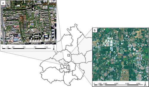
The urban area (662 × 528 pixel) covers Wudaokou commercial zone and parts of Tsinghua University in Beijing, covering an area of 1.4 km². The corresponding satellite image is acquired from WorldView-2 with 2-meter resolution. It contains vast artificial features, including buildings (like commercial buildings, apartments, residential buildings, and shantytowns) and roads, as well as natural landscapes like vegetation and waters. The farmland area (674 × 644 pixel) named Xiaotang Mountain is located in suburban area of Beijing with an area of 98 km². The image is obtained from Landsat 8 OLI_TRIS data, and its multispectral band is firstly pan-sharpened with the panchromatic bands to generate a relatively higher resolution, 15-meter. This area is a local farming village, which mainly contains farmlands, bare soil, residential buildings, experimental fields, roads and so on.

Methodology

Framework of self-adaptive segmentation

Self-adaptive segmentation (SAS) essentially belongs to variable-scale segmentation, with fully considering three factors which can influence segmentation scales: category system, surrounding contrast and internal heterogeneity.

Regular multiscale segmentations (DrăGuţ et al. 2014; Du et al. 2016), as seen in Equation 1, aim at minimizing the ${\delta }_{mul}$ value, which is defined as the average difference between inherent scale ($S_i$) of object $i$ and segmentation scale ($S_{seg}$). The segmentation scale here refers to a global one applied for all objects. SAS is also defined in a similar way in Equation 2. The only difference between them lies in the segmentation scale learned for each object $i$ , which is denoted by $S_{segi}$ . As a matter of fact, an individual segmentation scale is specifically designed for each object by selfhood scale estimation technique in SAS, aiming at minimizing the gap between segmentation and inherent scales. This scale-learning mechanism introduces human prior knowledge in training samples, which efficiently relieves the situation of unsupervised scale-selection in current segmentations (Zhang and Du 2016).

(1) ${\delta }_{mul}=\frac{{\sum }_{i=1}^N\left(S_{seg}-S_i\right)}{N}$(1)

(2) ${\delta }_{adp}=\frac{{\sum }_{i=1}^N\left(S_{segi}-S_i\right)}{N}$(2)

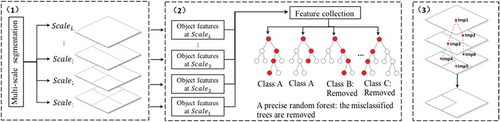
In general terms, our SAS segmentation method can be summarized as below: First, initial segments are produced by SWA method. It automatically generates segmentation results at continuous scales adapting to images’ characteristics without too much human interventions (Du et al. 2016). Then, based on the generated multiscale results, the optimum segmentation scale for each object can be estimated using selfhood scale learning method, which takes the category system, surrounding contrast and internal heterogeneity into consideration during supervised learning process (Zhang and Du 2016). Finally, neighbouring segments are iteratively and adaptively merged accordingly to the learned selfhood scales. The method will be outlined with more details in the following sections and flowchart (Figure 2).

Figure 2. Flow chart for SAS, including three steps: (a) producing continuous multiscale segments by SWA approach; (b) calculating features for each scale from the first step and combining them later to learn selfhood scales; (c) finishing the merging based on the learned selfhood scales and generating self-adaptive results.

Producing multiscale segments based on the improved SWA

The SWA method was first introduced by Sharon et al. (2006) for natural image segmentations. Since then, it has been employed by Wang, Wang, and Wu (2009) and more recently by Du et al. (2016) to automatically segment remote sensing images. As seen in Figure 3, it mainly consists of four steps: (1) Constructing fine-level graph. Each pixel/object in an image is represented as a node in the graph, and coupled to its four neighbours according to their similarity in the intensity level. (2) Creating coarser graph. The coarsening process continues recursively, aggregating collections of nodes into much fewer nodes in coarser-level graphs until only one node is left on the top graph, thus builds a pyramid of graphs bottom-up. Not only pixel-level but also large-scale measurements are incorporated into this continuing coarsening process to achieve better segmentation. (3) Evaluating segments’ saliency. A salient value is defined as the ratio between inter- and intra-segment heterogeneity, used to select the best segmentation (salient segments) among SWA’s multiscale results. A salient segment of the image is the one for which the similarity across its border is large, whereas within the segment is small. (4) Determining boundaries of salient segments by a top-down process.

Figure 3. Flow chart for Segmentation by Weighted Aggregation (SWA) approach (Sharon et al. 2006).

In order to improve the precision and efficiency of the existing SWA method, two important improvements have been made to it: First, large-scale features are taken fully use of to enrich feature measurements. Based on the previous work of Du et al. (2016), our study introduces abundant large-scale features, including mean spectrum, shape moment and variance of mean spectrum. In addition, filter response and orientation histogram are especially added to relieve the insufficiency situation of texture features, the conceptual bases and methodology implementations of which are well addressed in literature (Galun et al. 2003). Second, SWA’s efficiency is improved compared to the work of Du et al. (2016), which can hardly deal with large collections of remote sensing images. Accordingly, several modifications have also been made to the algorithm, which raises the efficiency dramatically.

Learning selfhood scale

The selfhood scale refers to a local optimal and self-adaptive segmentation scale of each pixel, which skills at self-adaptive segmentations and measuring local contexts of pixels (Zhang and Du 2016). It aims at bridging the gap between segmentation and inherent scales and improving segmentation results with prior knowledge. The detailed description of this learning process is illustrated in Figure 2(b). To learn selfhood scales from multiscale results produced by SWA, each scale is scored by feature importance firstly. Gini importance (Breiman 2001) derived from random forest is widely used to measure the feature importance, and the scale with the largest score is considered as the selfhood scale. In this article, three typical improvements have been made to the learning mechanism of selfhood scales.

Firstly, objects, instead of pixels, are employed as basic units for measuring selfhood scales. Even though theoretically speaking each pixel can have its own selfhood scale (Zhang and Du 2016), pixel-based selfhood scale usually leads to many salt and pepper phenomena in experiments, which does harm to subsequent merging results. As seen in Equation 3, $ScaleIm{p}_i\left(Objec{t}_p\right)$, the importance of the $i^{th}$ scale ($1\le i\le L$) for classifying $Objec{t}_p$, is the sum of the importance of all the features at the $i^{th}$ scale. Among all L scales, the most important scale with the largest $ScaleIm{p}_i\left(Objec{t}_p\right)$ is considered as the selfhood scale of $Objec{t}_p$, denoted by $Selfhoodscale\left(Objec{t}_p\right)$ (Equation 4).

(3) $ScaleIm{p}_i\left(Objec{t}_p\right)=\sum _{j}FeatureIm{p}_j\left(Pixe{l}_p\right)\left(j\in Scal{e}_i\right)$(3)

(4) $Selfhoodscale\left(Objec{t}_p\right)=argma{x}_{i=1}^{L}ScaleIm{p}_i\left(Objec{t}_p\right)$(4)

Besides, objects at the finest scale produced by SWA are used as basic units to calculate selfhood scales in this study for staying continuous homogeneity as much as possible. This modification can also reduce learning time remarkably.

Secondly, precise random forest instead of a fuzzy one is proposed in this study. As seen in Figure 2(b), existing learning mechanism always goes through all classification trees in the random forest to accumulate the decrease in Gini coefficients for measuring features’ importance, including those misclassified trees (labelled as class B or C). However, Gini importance is essentially used to assess feature contributions in classifying each object, and thus the decreases in Gini coefficients of misclassification trees should not be counted. As seen in Figure 2(b), only decreases of Gini coefficients in trees left behind (labelled as class A) are counted.

Thirdly, this study implements selfhood scale learning process based on RandomForestClassifier in Scikit-learn suit of python. As python provides us with marvellous parallel technique, it raises efficiency greatly and is also of great significance to process massive remote sensing images.

Self-adaptive merging to generate self-adaptive results

With the preceding selfhood scales, each object can find its appropriate segmentation scale and segments among multiscale SWA results. Then self-adaptive merging method can identify objects of the same categories consistently. As depicted in Figure 4(a), is a simplified tree representation of self-adaptive merging, and (b) shows the concrete merging process.

Figure 4. Self-adaptive merging based on learned selfhood scales. (a) is the simplified tree representation of the workflow for self-adaptive merging. Each object in level 0 represented by leaf node searches for an appropriate segment bottom-up according to the learned selfhood scale, indicated by the corresponding color. Then the tree splits into subtrees with father nodes representing new segments. (b) is the concrete merging illustration. It shows the merging process of objects step by step.

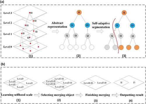
In Figure 4(a), objects at level 0 are regarded as basic units for learning selfhood scales; levels 1–3 are multiscale results produced by SWA. The goal of SAS is to merge the fragmentary objects at local appropriate scales. Firstly, the pyramid structure of multiscale results (in Figure 4(a)(1)) is represented by a tree in Figure 4(a)(2), with leaf nodes corresponding to image segments in level 0, father nodes corresponding to segments in upper coarse-scale graphs. SWA finally outputs each coarse-scale result as one segmentation result (nodes with the same colors in Figure 4(a)(2)), only taking relations of the same level nodes into consideration while ignoring important father-son relations exiting in this tree. Contrarily, SAS considers both two kinds of relations. It searches up the family tree (Figure 4(a)(3)) and finds the appropriate segmentation scale (farther nodes) for each object (leaf nodes). For example, in Figure 4(a)(3), some leaf nodes (the grey) choose level 1 as optimum segmentation scale and others (the orange red) select level 3 as ideal ones. Finally, according to the learned selfhood scales, objects merge automatically to create new aggregates. The tree then splits into two subtrees with consideration of both horizontal and vertical inter-node relationships. Each tree of them represents one segment.

Figure 4(b) is the concrete merging process consisting of four steps: (1) Assigning selfhood scale for each object. As depicted in Figure 4(b)(1), two objects’ selfhood scales are labelled as “Level 1” and others as “Level 3.” (2) Selecting merging segments. According to the selfhood scales obtained in (1), each object in level 0 can find appropriate segments according to its selfhood scale. For example, as for objects whose selfhood scales are “Level 1,” the algorithm searches for corresponding segments in Figure 4(a)(1), i.e., I1, so that they are relabelled as Level 1-I1. (3) Merging objects with the same labels. As seen in the figure, objects labelled as Level 1-I1 can be merged together as one segment, and objects labelled as Level 3-I1 will be merged into another one. (4) Sorting out the segments with new labels and then output results.

Evaluation

This study combines qualitative and quantitative methods to fully evaluate segmentation results. Firstly, visual interpretation is used to estimate the local segmentation quality (Giora and Casco 2007). Since the operators are equipped with abundant prior knowledge, it is much easier and more flexible for them to distinguish the better ones. However, this can be also a double-edged sword for bringing in many subjective judgements. Furthermore, restricted by human’s daily time and energy, this method can be hardly applied to large-scale evaluations.

For quantitative evaluation, both unsupervised (Global Score) and supervised methods (Geometry-based method) are introduced to evaluate segmentation results globally. Global score (GS) is an unsupervised evaluation method of segmentation quality proposed by Johnson and Xie (2011) with consideration of global intra-segment and inter-segment heterogeneity measures, which are calculated by weighted variance and Moran’s I. The supervised geometry-based method compares the geometry between reference polygons and segments, and then quantitatively measures the degrees of over-segmentation and under-segmentation. Three measurements are employed in this study including over-segmentation (Osg), under-segmentation (Usg) and root mean square (RMS) (Clinton et al. 2010; Guo and Du 2017). RMS is a combination index of Osg and Usg, which can be used to measure the overall segmentation quality. For all indexes, the smaller, the better. Accordingly, both local and global evaluations, unsupervised and supervised evaluations are considered in our quality estimation, providing a comprehensive view on segmentation accuracies.

Experiments and analyses

Procedure for experiments

The experiments mainly contain three parts listed as below: Firstly, SWA was used to segment remote sensing images into multiscale objects. Since the available SWA program designed for remote sensing images was time consuming (Du et al. 2016), this study improved its efficiency at first. Based on that, selfhood scales were learned for subsequent self-adaptive merging (Section 4.2) to generate SAS results. Then, the results were compared with SWA results in section 4.3. Finally, our method was further evaluated with a state-of-the-art method, the mean shift segmentation, in section 4.4, which has been widely explored in previous studies (Comaniciu 2003; Comaniciu and Meer 2002; Comaniciu, Ramesh, and Meer 2000, 2001; Ming et al. 2012, 2015).

Self-adaptive segmentation results

SWA segmentation results

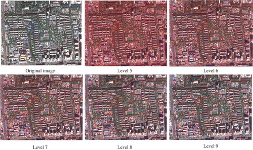
Firstly, for urban area (Figure 1(a)), SWA produced 16 levels (scales) of segmentation results automatically in about 30s, which significantly reduced the time consumption from days to seconds compared to the work in Du et al. (2016). Due to the length limitation of this paper, only levels 5–9 were shown in Figure 5. As can be seen, SWA produced multiscale results ranging from over-segmented results to under-segmented ones with no need to set parameters manually. It was obvious that levels 1–4 were severely over-segmented while levels 10–16 were under-segmented. For urban area, the optimum segmentation scales fell within levels 5–9, thus they were used to learn selfhood scales for geographic objects afterwards.

Figure 5. Multiscale results generated by SWA approach for urban area.

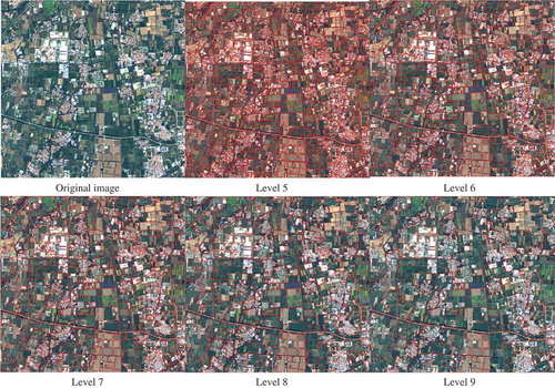
In farmland study area, 14 levels were generated from SWA program, which differed from those in urban area (16 levels). This was mainly because SWA could produce multiscale results adapting to image property. Since the results below level 5 and above level 9 were obviously over- or under-segmented, the similar decision was made to farmland area: levels 5–9 were kept (Figure 6) for further selfhood scale learning process.

Figure 6. Multiscale results generated by SWA approach for farmland area.

Selfhood scale learning results

Based on continuous multiscale results in SWA (levels 5–9), the selfhood scale was learned for each object. For each scale level, 14 features were firstly extracted to characterize objects including averaged spectrums, shape index, area, density, as well as the derivative features from Gray Level Co-occurrence Matrix (GLCM) since they were proved to be effective in previous studies (Nevatia and Babu 1980; Zhang and Du 2016). Then all 70 (14 features*5 levels) features could be obtained and employed in selfhood scale learning. The learning results were presented in Figure 7. Each basic unit was identified by its selfhood scale (ranging from level 5 to level 9) colored differently in the figure.

Figure 7. Selfhood scale learning results for (a) urban area and (b) farmland area. Each object was colored differently according to its selfhood scale learned from multiscale SWA results, ranging from level 5 to level 9.

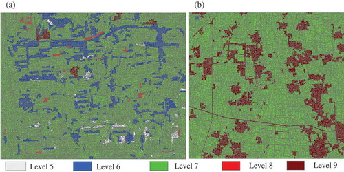
As depicted in Figure 7(a) in urban area, a majority of objects selected level 6 or level 7 as their selfhood scales, and the others took levels 5, 8, and 9. Seeing from the spatial distribution of learned selfhood scales, middle scales (level 6 and level 7) were favored by most geographical objects, which seemed to follow some kind of normal distribution. However, in Figure 7(b), it was very clear that selfhood scales for farmland area mainly distributed on levels 7 and 9, while a small number of entities considered level 6 as their selfhood scales and no object took level 5 or level 8 as their selfhood scales. These results indicated that selfhood scales for farmland objects were greatly focused, mainly in relatively large scales, like level 7 and level 9.

Selfhood scales were then categorized by classes, and the detailed statistics were reported in Tables 1 and 2. As Table 1 indicated, selfhood scales in urban area could change among different categories. For example, selfhood scales for green vegetation concentrated on level 6 while those for other classes were on level 7. Due to diverse surroundings in the image, different objects within the same class might also have distinctive selfhood scales. Taking waters for instance, 56.41% objects considered the scale of level 7 while 28.21% selected level 6 as selfhood scales, and the rest fell in level 5. Therefore, segmentation scales for waters actually distributed on three continuous scales (level 5, level 6 and level 7). These conclusions are exactly consistent with the research of Zhang and Du (2016): both the categories and surroundings can impact the choice of selfhood scales.

Table 1. The per-category proportions of different selfhood scales in urban area.

Proportion (%)	Level 5	Level 6	Level 7	Level 8	Level 9
Bright building	1.52	1.38	97.00	0.10	0
Dark building	6.48	19.44	74.07	0	0
Shadow	16.09	10.12	73.79	0	0
Road	0	0.35	99.65	0	0
Green vegetation	2.18	56.78	41.04	0	0
Red vegetation	4.09	9.21	65.98	0.51	20.20
Water	15.38	28.21	56.41	0	0
Total	6.53	17.93	72.56	0.09	2.89

The bold numbers represent the largest proportion for each category.

Table 2. The per-category proportions of different selfhood scales in farmland area.

Proportion (%)	Level 5	Level 6	Level 7	Level 8	Level 9
Bright building	0	0	98.59	0	1.41
Mixed residential area	0	0	8.23	0	91.77
Dark green farmland	0	0.88	98.83	0	0.29
Light green farmland	0	0	100.00	0	0
Bare soil	0	0	100.00	0	0
Road	0	0	11.11	0	88.89
Total	0	0.15	69.46	0	30.39

The bold numbers represent the largest proportion for each category.

In farmland area (in Table 2), selfhood scales for different categories differed greatly, but varied a little within the same category. For example, selfhood scales of bright buildings, dark green farmlands, light green farmlands and bare soil focused on level 7, but those for mixed residential areas and roads were on level 9. However, as for the same category, the majority of the entities selected one representative scale as their selfhood scale. For example, in light green farmlands and bare soil, all entities took level 7 as their selfhood scale; 98.59% bright buildings and 98.83% dark green farmlands chose level 7 too; 91.77% mixed residential areas and 88.89% roads selected level 9 as their selfhood scales. It was because in farmland area, types of geographical objects tended to be simple and clustered with similar individual features and surroundings, thus they could be well segmented at the same scales.

Self-adaptive merging

Based on selfhood scales learned in Figure 7, each object went through multiscale results in SWA to search for the optimum segment in corresponding scales. Then the multiscale segments were merged together by self-adaptive merging technique described in section 3.4. The SAS results for urban area and farmland area can be seen in Figures 8(b) and 10(b) respectively. Since SWA was proved to be an efficient approach by Du et al. (2016), SAS was firstly compared with its multiscale results (levels 5–9) in section 4.3.

Figure 8. A comparison between SWA and SAS results in urban area. (a) The original image and (b) the SAS result. A heterogeneous region, marked with yellow rectangle, is chosen to visually compare the six kinds of segmentation results at (c) level 5, (d) level 6, (e) level 7, (f) level 8, (g) level 9 of SWA results and (h) SAS result.

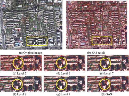
Figure 9. The manually delineated reference data used in geometry-based evaluation for (a) urban area and (b) farmland area.

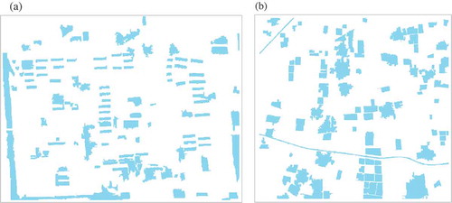
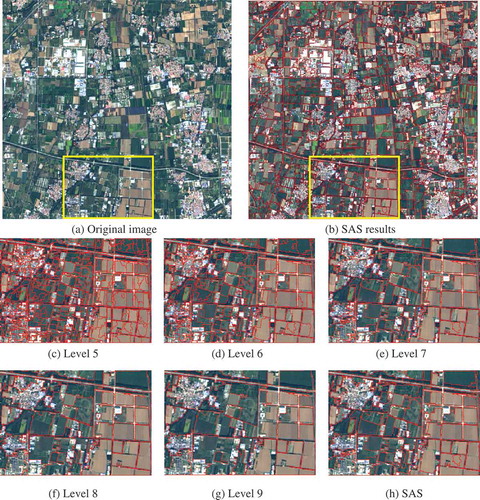
Figure 10. A comparison between SWA and SAS results in farmland area. (a) The original image and (b) the SAS result. A heterogeneous region, marked with yellow rectangle, is chosen to visually compare the six kinds of segmentation results at (c) level 5, (d) level 6, (e) level 7, (f) level 8, (g) level 9 of SWA results and (h) SAS result.

A comparison of self-adaptive and SWA result

Self-adaptive segmentation vs. SWA in urban area

As demonstrated in Figure 8, (a) was the original image, (b) represented the corresponding SAS result. A heterogeneous region (marked with a yellow rectangle) was chosen for visual interpretation. It contained diverse entities, e.g., buildings, vegetation, shadow and bare soil. Since vegetation and bare soil scattered across the study area and mixed with buildings and shadow, it would be challenging for us to distinguish them accurately.

At level 5, buildings, vegetation and shadow were all under-segmented. While at level 6, shadow obtained good segmentation results, the majority of which were distinguished from buildings with great integration. As mentioned above, vegetation was usually mixed with buildings and shadow, which brought lots of difficulties into segmentation. In the results of level 6, some vegetation was over-segmented while the others was under-segmented due to its fragmented distribution. While at level 7, over-segmentation of buildings had eased somewhat, but under-segmentation emerged in vegetation and shadow. The under-segmentation got more and more serious in level 8 and level 9. However, compared with SWA results, SAS (Figure 8(h)) extracted buildings, vegetation, shadow and bare soil completely from the original image with greater integrity. Took a small shadow area (marked with a yellow circle) for example. It was over-segmented in level 5, and under-segmented in levels 6–9 (mixed with vegetation). However, in the SAS result, this shadow was delineated accurately as one complete segment.

In addition to qualitative comparison, quantitative one was also necessary. Both unsupervised and supervised evaluations were included in this comparison. For unsupervised evaluation, global score ($GS$) index was calculated. While in supervised one, geometry-based evaluation was introduced in this comparison. Manually delineated polygons (Figure 9) were employed as reference to evaluate the segmentation quality. Based on them, three evaluation indexes (OSeg, USeg and RMS) could be calculated for measuring segmentation accuracies of levels 5–9 in SWA results and SAS results, and the statistics were reported in Table 3.

Table 3. Evaluation statistics of quantitative comparisons between SWA and SAS results (in urban area).

Methods	Scale	GS	OSeg	USeg	RMS
SWA	Level 5	0.463	0.731	0.010	0.518
	Level 6	0.410	0.467	0.065	0.370
	Level 7	0.330	0.227	0.160	0.267
	Level 8	0.373	0.183	0.445	0.430
	Level 9	0.433	0.184	0.607	0.540
SAS	-	0.328	0.296	0.044	0.236

The bold numbers represent the best segmentation results for each method.

As shown in the table, with the increasing of scale, $GS$ value for SWA increased firstly and decreased afterwards. It achieved the minimum at level 7 (0.330), implying the optimum segmentation scale in SWA. However, the value was still larger than that of SAS, which obtained a relatively lower value of 0.328, indicating further improvement of multiscale segmentation.

In the geometry-based evaluation, with the increment of scale, USeg got larger while OSeg became smaller, which indicated more under-segmentations and few over-segmentations. It was exactly consistent with common cognition. RMS could be used to assess the overall quality of segmentation. It decreased firstly, and went up afterwards. Since from level 5 to level 7, over-segmentation gradually disappeared and under-segmentation had not been universal, thus segmentation quality kept going higher. With the scale keeping increasing (levels 8–9), under-segmentation overweighed over-segmentation leading to lower and lower quality. RMS gained the minimum at level 7, therefor it was considered as the optimum segmentation scale for SWA, which had both relatively lower OSeg and USeg values.

However, SAS exposed greater precision than SWA at level 7 for obtaining smaller RMS value (0.236). This improvement was mainly due to the decrease in USeg, indicating less under-segmented objects. It also indicated that SAS was effective in relieving under-segmentation and optimizing local segmentation, which was consistent with conclusions in qualitative comparison. To sum up, SAS achieved better results than SWA in multiscale segmentation as demonstrated in both evaluations.

Self-adaptive segmentation vs. SWA in farmland area

Based on the learned selfhood scales presented in Figure 7(b), the SAS results were generated in Figure 10(b). A typical area marked with yellow rectangle was chosen for visual interpretation. As seen in SAS results, mixed residential areas and roads tended to select large scale (level 9) as their selfhood scales, so segments at level 9 for mixed residential areas and roads were expressed in final SAS results. With large segmentation scales, roads and mixed residential areas were segmented out with great integration. On the contrary, vegetation, bare soil, and bright buildings were segmented with smaller scales, also producing decent segmentation results. Therefore, SAS outperformed SWA by reference to overall accuracy, as it assigned an appropriate segmentation scale for each object, which exactly bridged the gap between segmentation and inherent scales.

In addition, quantitative evaluation statistics were shown in Table 4, including GS, OSeg, USeg and RMS. It reported that level 7 had the minimum GS and RMS, implying the optimum result among SWA results. The GS and RMS of SAS results were 0.202 and 0.167 respectively, which were significantly smaller than those of SWA results. Moreover, both OSeg and USeg of SAS showed in the table were smaller than corresponding statistics of SWA. These evidences further proved that SAS was more effective than SWA in segmenting the farmland area.

Table 4. Evaluation statistics of quantitative comparisons between SWA and SAS results (in farmland area).

Methods	Scale	GS	OSeg	USeg	RMS
SWA	Level 5	0.308	0.794	0.010	0.562
	Level 6	0.268	0.545	0.029	0.401
	Level 7	0.227	0.237	0.086	0.218
	Level 8	0.233	0.101	0.365	0.326
	Level 9	0.251	0.025	0.637	0.466
SAS	-	0.202	0.147	0.096	0.167

The bold numbers represent the best segmentation results for each method.

A comparison of self-adaptive and mean shift segmentation result

Self-adaptive segmentation vs. mean shift in urban area

SAS was further compared with mean shift method in Figure 11. In this experiment, the mean shift results were generated by ArcGIS software with default parameters (Spectral Detail:15.5, Spatial Detail:15, Minimum Segment Sizes in Pixels:20). Since in urban area, buildings, vegetation, shadow, and roads were scattered, it would be challenging for us to separate them. As shown in the Figure 11, mean shift method generated rather broken results from visual perception. Although buildings were well segmented as complete ones even better than those in SAS results, other objects were over-segmented, especially for vegetation and shadow. This study even experimented on many parameter pairs to find the appropriate scale for all objects but failed. This attempt indicated that mean shift method could hardly balance between spectral detail and spatial detail, which also hindered the realization of automatic scale-selection.

Figure 11. A comparison between SWA and mean shift results in urban area.

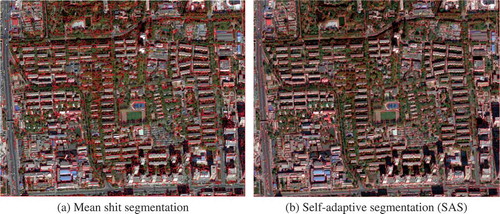
The similar conclusion could also be drawn from the quantitative evaluation in Table 5. Both Oseg (0.304) and Useg (0.163) values of mean shift were larger than those of SAS, implying substantial over-segmentations and under-segmentations in mean shift result. Comprehensively speaking, SAS obtained much better segmentation results than mean shift, as its GS (0.328) and RMS (0.236) were much smaller than those of mean shift, which possibly attributed to the prior-knowledge driven scale estimation process introduced in SAS approach. Thanks to the selfhood scale technique, it allowed us to assign appropriate segmentation scales for interesting objects in the image. Thus, more and more objects could be segmented in a scale much closer to its inherent scale with great integrity and precision.

Table 5. Evaluation statistics of quantitative comparisons between mean shift and SAS results (in urban area).

Methods	GS	OSeg	USeg	RMS
Mean shift	0.452	0.304	0.163	0.389
SAS	0.328	0.296	0.044	0.236

Self-adaptive segmentation vs. mean shift in farmland area

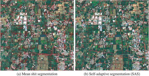
Then in farmland area, the SAS result was compared with mean shift results for further validation. Similar to situations in urban area, this study also explored many parameter pairs (including spectral detail, spatial detail and minimum segment sizes in pixels) to find the appropriate one at first, but the results did not improve a lot and the default one was adopted in the experiment at last. In Figure 12 (a), it was clear that some farmlands were completely segmented, but the others were still mixed together. Owing to the complexity of farmland areas, mean shift method could hardly segment them as complete individuals. It could be difficult for it to make a right choice of appropriate segmentation scales adapting to diverse scenes. Thus, in the segmentation result of mean shift, both over-segmentations and under-segmentations were universal. However, in the SAS situation, these phenomena were relatively relieved. Majority farmlands were segmented well, and the roads and mixed residential areas were distinguished accurately as what we initially expected: the roads should better be generated as complete ones, and the buildings in residential areas ought to be delineated as separable patches. With respect to quantitative evaluation results in Table 6, the SAS was also proved to be better than mean shift for obtaining much lower statistic values in all indexes, which demonstrated the significant advantages of SAS method.

Table 6. Evaluation statistics of quantitative comparisons between mean shift and SAS results (in farmland area).

Methods	GS	OSeg	USeg	RMS
Mean shift	0.447	0.325	0.124	0.342
SAS	0.202	0.147	0.096	0.167

Figure 12. A comparison between SWA and mean shift results in farmland area.

Discussions

Based on the qualitative and quantitative comparisons between SWA and mean shift segmentation in section 4, the SAS method is proved to have following characteristics which makes it superior in multiscale segmentation:

1. The SAS can produce segmentation results closer to inherent scales of geographical entities. Thanks to the SWA incorporated in this study, the SAS method is implemented on continuous multiscale results (Du et al. 2016; Sharon et al. 2006), which makes it distinct from traditional methods, e.g., multiresolution segmentation (Baatz and Schape 2000; DrăGuţ et al. 2014) or mean shift method (Ming et al. 2012, 2015). The continuous multiscale results generated by SWA are more similar to what in natural cases, which lays a solid foundation for further analysis. Besides, SAS adopts a novel scale estimation technique, i.e., the selfhood scale learning mechanism, which perfectly bridges the gap between segmentation scales and inherent ones. Selfhood scales are local variables adapting to the local variations of geographic environment (Zhang and Du 2016) which can intelligently decide the right segmentation scale for each object.

2. As demonstrated in section 4, SAS achieves greater performance than SWA and mean shift method, which may also attribute to its supervised characteristic. Most available multiscale segmentation methods are unsupervised ones (DrăGuţ et al. 2014; Ming et al. 2012), which may limit the usage of prior knowledge or expert knowledge in object segmentation. In SAS’ situation, it makes full use of prior knowledge in following two ways: Firstly, SWA involves a top-down process, expressing prior knowledge about geographic objects and information on contexts and attentions, to improve segmentation quality through modifying similarity between neighboring objects in the adaptive structure (Du et al. 2016; Sharon et al. 2006). In addition, selfhood scales can be automatically learned from multiscale segmentation results with a few training samples, thus they can be easily obtained and learned based on human knowledge (Zhang and Du 2016). It is totally different from existing scale estimation methods (DrăGuţ et al. 2014; Smith 2010), which can only produce data-driven scales. Accordingly, the implementation of SAS is actually more consistent with human cognition.

3. The SAS is validated to be stable and transferable to more applications. As demonstrated in section 4, the proposed SAS method is conducted in two different areas and with two data sets to evaluate its effectiveness. Both results show that the SAS achieves greater performance in these areas for obtaining better accuracies. It clearly indicates the stability and adaptability of SAS to a broader range of applications.

The limitation of the proposed SAS method lies in that the selfhood scale learning process is not stable enough. It can be influenced by parameters of the random forest (Zhang and Du 2016). A quantitative relationship between them may be estimated in later research so that the selfhood learning process can be optimized further. In addition, in the future work, the robustness and universality of the SAS program are expected to be improved to handle a large number of remote sensing data and provided as an open source package available to more researchers.

Conclusions

It has been shown that existing multiscale segmentations (Baatz and Schape 2000; Du et al. 2016) are not satisfactory due to the significant gap between segmentation scales and the inherent scales of geographic entities, which have been experimentally validated in section 4. This study proposes a self-adaptive segmentation (SAS) method aiming at solving the scale uncertainty in segmentation, and further compares it with SWA (Du et al 2016) and mean shift method (Comaniciu 2003; Comaniciu and Meer 2002; Comaniciu, Ramesh, and Meer 2000, 2001). Accordingly, three conclusions have been drawn.

First of all, the proposed SAS method with optimized selfhood scale leaning method is effective in improving multiscale segmentation according to the evaluations in section 4. Then, the proposed segmentation method shows strong adaptability to different data sources and study areas, and the improvement is more significant in farmland area. Finally, SAS produces more accurate segmentation results compared with SWA and mean shift method, attributing to the contribution of selfhood scales. These conclusions are totally unique in three ways. First, the SAS method is firstly proposed and clearly clarified in this study. It is distinct from existing unsupervised multiscale methods (Baatz and Schape 2000; Comaniciu 2003; DrăGuţ et al. 2014; Du et al. 2016; Johnson and Xie 2011; Yuan and Barner 2006). Second, an improved selfhood scale learning method successfully realizes local optimization for each object rather than for global ones (DrăGuţ et al. 2014) or local regions (Zhang, Feng et al. 2015), which can be meaningful for connecting segmentation scales and inherent scales in minor geographical units. Third, the SWA technique employed in SAS method is of great significance for producing segmentation results at continuous scales automatically (Du et al. 2016; Sharon et al. 2006) while traditional ones focus on discrete scales (DrăGuţ et al. 2014; Zhang and Du 2016). In summary, the proposed SAS is complementary to existing multiscale segmentations with strong adaptability to different study areas and datasets.

Disclosure statement

No potential conflict of interest was reported by the authors.

References

- Baatz, M., and A. Schape. 2000. “Multiresolution Segmentation: An Optimization Approach for High Quality Multi-Scale Image Segmentation.” In: Angewandte Geographische Informationsverarbeitung XII, edited by J. Strobl, T. Blaschke, and G. Griesebner, 12–23. Heidelberg: Wichmann-Verlag.
- Blaschke, T., G. J. Hay, M. Kelly, S. Lang, P. Hofmann, E. Addink, R. Queiroz Feitosa, et al. 2014. “Geographic Object-Based Image Analysis–Towards a New Paradigm.” ISPRS Journal Photogramm Remote Sens 87 :180–191. doi:10.1016/j.isprsjprs.2013.09.014.
- Boykov, Y. Y., and M. P. Jolly. 2001. “Interactive Graph Cuts for Optimal Boundary, and Region Segmentation of Objects in ND Images”. Proceedings Eighth IEEE International Conference on Computer Vision, Vancouver, BC, Canada, July 7-14, 105–112. doi:10.1109/iccv.2001.937505.
- Breiman, L. 2001. “Random Forests.” Machine Learning 45: 5–32. doi:10.1023/A:1010933404324.
- Chen, G., Q. Weng, G. J. Hay, and Y. He. 2018. “Geographic Object-Based Image Analysis (Geobia): Emerging Trends and Future Opportunities.” Giscience & Remote Sensing 55 (2): 159–182. doi:10.1080/15481603.2018.1426092.
- Cheng, H. D., and Y. Sun. 2000. “A Hierarchical Approach to Color Image Segmentation Using Homogeneity.” IEEE Transactions on Image Processing 9 (12): 2071–2082. doi:10.1109/83.887975.
- Cheng, J., Y. Bo, Y. Zhu, and X. Ji. 2014. “A Novel Method for Assessing the Segmentation Quality of High-Spatial Resolution Remote-Sensing Images.” International Journal of Remote Sensing 35 (10): 3816–3839. doi:10.1080/01431161.2014.919678.
- Clinton, N., A. Holt, J. Scarborough, L. Yan, and P. Gong. 2010. “Accuracy Assessment Measures for Object-Based Image Segmentation Goodness.” Photogrammetric Engineering and Remote Sensing 76 (3): 289–299. doi:10.14358/pers.76.3.289.
- Comaniciu, D. 2003. “An Algorithm for Data-Driven Bandwidth Selection.” IEEE Transactions on Pattern Analysis and Machine Intelligence 25 (2): 281–288. doi:10.1109/tpami.2003.1177159.
- Comaniciu, D., and P. Meer. 2002. “Mean Shift: A Robust Approach toward Feature Space Analysis.” IEEE Transactions on Pattern Analysis and Machine Intelligence 24 (5): 603–619. doi:10.1109/34.1000236.
- Comaniciu, D., V. Ramesh, and P. Meer. 2000. “Real-Time Tracking of Non-Rigid Objects Using Mean Shift.” Proceedings IEEE Conference on Computer Vision and Pattern Recognition, Hilton Head Island, SC, USA, June 15, 142–149. doi:10.1109/cvpr.2000.854761.
- Comaniciu, D., V. Ramesh, and P. Meer. 2001. “The Variable Bandwidth Mean Shift and Data-Driven Scale Selection”. Proceedings Eighth IEEE International Conference on Computer Vision, Vancouver, BC, Canada, July 7-14, 438–445. doi:10.1109/iccv.2001.937550.
- DrăGuţ, L., D. Tiede, and S. R. Levick. 2010. “ESP: A Tool to Estimate Scale Parameter for Multiresolution Image Segmentation of Remotely Sensed Data.” International Journal of Geographical Information Science 24 (6): 859–871. doi:10.1080/13658810903174803.
- DrăGuţ, L., O. Csillik, C. Eisank, and D. Tiede. 2014. “Automated Parameterisation for Multiscale Image Segmentation on Multiple Layers.” ISPRS Journal of Photogrammetry and Remote Sensing 88: 119–127. doi:10.1016/j.isprsjprs.2013.11.018.
- Du, S., Z. Guo, W. Wang, L. Guo, and J. Nie. 2016. “A Comparative Study of the Segmentation of Weighted Aggregation and Multiresolution Segmentation.” GIScience and Remote Sensing 53 (5): 651–670. doi:10.1080/15481603.2016.1215769.
- Eriksson, A. P., C. Olsson, and F. Kahl. 2011. “Normalized Cuts Revisited: A Reformulation for Segmentation with Linear Grouping Constraints.” Journal of Mathematical Imaging and Vision 39 (1): 45–61. doi:10.1109/iccv.2007.4408958.
- Galun, M., E. Sharon, R. Basri, and A. Brandt. 2003. “Texture Segmentation by Multiscale Aggregation of Filter Responses and Shape Elements.” IEEE International Conference on Computer Vision, Nice, October 13–16, 716–723. doi:10.1109/iccv.2003.1238418.
- Georganos, S., T. Grippa, S. Vanhuysse, M. Lennert, M. Shimoni, S. Kalogirou, and E. Wolff. 2017. “Less Is More: Optimizing Classification Performance through Feature Selection in a Very-High-Resolution Remote Sensing Object-Based Urban Application.” GIScience and Remote Sensing 55 (2): 221–242. doi:10.1080/15481603.2017.1408892.
- Giora, E., and C. Casco. 2007. “Region-And Edge-Based Configurational Effects in Texture Segmentation.” Vision Research 47 (7): 879–886. doi:10.1016/j.visres.2007.01.009.
- Grady, L. 2006. “Random Walks for Image Segmentation.” IEEE Transactions on Pattern Analysis and Machine Intelligence 28 (11): 1768–1783. doi:10.1109/tpami.2006.233.
- Grybas, H., L. Melendy, and R. G. Congalton. 2017. “A Comparison of Unsupervised Segmentation Parameter Optimization Approaches Using Moderate- and High-Resolution Imagery.” GIScience and Remote Sensing 54 (4): 515–533. doi:10.1080/15481603.2017.1287238.
- Guo, Z., and S. Du. 2017. “Mining Parameter Information for Building Extraction and Change Detection with Very High Resolution Imagery and GIS Data.” GIScience and Remote Sensing 54 (1): 38–63. doi:10.1080/15481603.2016.1250328.
- Guo, Z., S. Du, M. Li, and W. Zhao. 2016. “Exploring GIS Knowledge to Improve Building Extraction and Change Detection from VHR Imagery in Urban Areas.” International Journal of Image and Data Fusion 7 (1): 42–62. doi:10.1080/19479832.2015.1051138.
- Han, M., C. Zhang, and Y. Zhou. 2018. “Object-Wise Joint-Classification Change Detection for Remote Sensing Images Based on Entropy Query-By Fuzzing ARTMAP.” GIScience and Remote Sensing 55 (2): 265–284. doi:10.1080/15481603.2018.1430100.
- Hay, G. J., and G. Castilla. 2008. “Geographic Object-Based Image Analysis (GEOBIA): A New Name for A New Discipline.” In: Object Based Image Analysis, edited by T. Blaschke, S. Lang, and G. Hay, 93–112. Berlin: Springer-Verlag.
- Hay, G. J., T. Blaschke, D. J. Marceau, and A. Bouchard. 2003. “A Comparison of Three Image- Object Methods for the Multiscale Analysis of Landscape Structure.” ISPRS Journal of Photogrammetry and Remote Sensing 57 (5–6): 327–345. doi:10.1016/S0924-2716(02)00162-4.
- Ion, A., W. G. Kropatsch, and Y. Haxhimusa. 2006. “Considerations regarding the Minimum Spanning Tree Pyramid Segmentation Method.” In: Lecture Notes in Computer Science, edited by A. Ion, W. G. Kropatsch, and Y. Haxhimusa, 182–190. Berlin: Springer-Verlag.
- Johansen, K., N. Sallam, A. Robson, P. Samson, K. Chandler, L. Derby, A. Eaton, and J. Jennings. 2017. “Using Geoeye-1 Imagery for Multi-Temporal Object-Based Detection of Canegrub Damage in Sugarcane Fields in Queensland, Australia.” GIScience and Remote Sensing 55 (2): 285–305. doi:10.1080/15481603.2017.1417691.
- Johnson, B., and Z. Xie. 2011. “Unsupervised Image Segmentation Evaluation and Refinement Using a Multiscale Approach.” ISPRS Journal of Photogrammetry and Remote Sensing 66 (4): 473–483. doi:10.1016/j.isprsjprs.2011.02.006.
- Kavzoglu, T., M. Y. Erdemir, and H. Tonbul. 2017. “Classification of Semiurban Landscapes from VHR Satellite Images Using a Novel Regionalized Multi-Scale Segmentation Approach.” Journal of Applied Remote Sensing 11 (3): 1. doi:10.1117/1.JRS.11.035016.
- Liu, T., A. Abd-Elrahman, J. Morton, and V. L. Wilhelm. 2018. “Comparing Fully Convolutional Networks, Random Forest, Support Vector Machine, and Patch-Based Deep Convolutional Neural Networks for Object-Based Wetland Mapping Using Images from Small Unmanned Aircraft System.” GIScience and Remote Sensing 55 (2): 243–264. doi:10.1080/15481603.2018.1426091.
- Lu, B., and Y. He. 2017. “Optimal Spatial Resolution of UAV-acquired Imagery for Species Classification in a Heterogeneous Grassland Ecosystem.” GIScience and Remote Sensing 55 (2): 205–220. doi:10.1080/15481603.2017.1408930.
- Meinel, G., and M. Neubert. 2004. “A Comparison of Segmentation Programs for High Resolution Remote Sensing Data.” International Archives of Photogrammetry and Remote Sensing 35: 1097–1105.
- Ming, D., J. Li, J. Wang, and M. Zhang. 2015. “Scale Parameter Selection by Spatial Statistics for GeOBIA: Using Mean-Shift Based Multiscale Segmentation as an Example.” ISPRS Journal of Photogrammetry and Remote Sensing 106: 28–41. doi:10.1016/j.isprsjprs.2015.04.010.
- Ming, D., T. Ci, H. Cai, L. Li, C. Qiao, and J. Du. 2012. “Semivariogram-Based Spatial Bandwidth Selection for Remote Sensing Image Segmentation with Mean-Shift Algorithm.” IEEE Geoscience and Remote Sensing Letters 9 (5): 813–817. doi:10.1109/lgrs.2011.2182604.
- Nevatia, R., and K. R. Babu. 1980. “Linear Feature Extraction and Description.” Computer Graphics and Image Processing 13 (3): 257–269. doi:10.1016/0146-664x(80)90049-0.
- Platt, R. V., and L. Rapoza. 2008. “An Evaluation of an Object-Oriented Paradigm for Land Use/Land Cover Classification.” The Professional Geographer 60 (1): 87–100. doi:10.1080/00330120701724152.
- Santana, E. F., L. V. Batista, R. M. D. Silva, and C. A. G. Santos. 2014. “Multispectral Image Unsupervised Segmentation Using Watershed Transformation and Cross-Entropy Minimization in Different Land Use.” GIScience and Remote Sensing 51 (6): 613–629. doi:10.1080/15481603.2014.980095.
- Sharon, E., A. Brandt, and R. Basri. 2000. “Fast Multiscale Image Segmentation.” IEEE Conference on Computer Vision and Pattern Recognition, Hilton Head Island, SC, June 13–15, 70–77. doi:10.1109/cvpr.2000.855801.
- Sharon, E., M. Galun, D. Sharon, R. Basri, and A. Brandt. 2006. “Hierarchy and Adaptivity in Segmenting Visual Scenes.” Nature 442: 810–813. doi:10.1038/nature04977.
- Shi, J., and J. Malik. 2000. “Normalized Cuts and Image Segmentation.” IEEE Transactions on Pattern Analysis and Machine Intelligence 22: 888–905. doi:10.1109/34.868688.
- Smith, A. 2010. “Image Segmentation Scale Parameter Optimization and Land Cover Classification Using the Random Forest Algorithm.” Journal of Spatial Science 55: 69–79. doi:10.1080/14498596.2010.487851.
- Wang, A., S. Wang, and H. Wu. 2009. “Multiscale Segmentation of High Resolution Satellite Imagery by Hierarchical Aggregation.” Geomatics and Information Science of Wuhan University 34 (9): 1055–1058. in Chinese.
- Witharana, C., W. B. Ouimet, and K. B. Johnson. 2018. “Using LiDAR and GEOBIA for Automated Extraction of Eighteenth-Late Nineteenth Century Relict Charcoal Hearths in Southern New England.” GIScience and Remote Sensing 55 (2): 183–204. doi:10.1080/15481603.2018.1431356.
- Wuest, B., and Y. Zhang. 2009. “Region Based Segmentation of QuickBird Multispectral Imagery through Band Ratios and Fuzzy Comparison.” ISPRS Journal of Photogrammetry and Remote Sensing 64 (1): 55–64. doi:10.1016/j.isprsjprs.2008.06.005.
- Xu, Y., and E. C. Uberbacher. 1997. “2D Image Segmentation Using Minimum Spanning Trees.” Image and Vision Computing 15: 47–57. doi:10.1016/S0262-8856(96)01105-5.
- Yang, J., Y. He, and J. Caspersen. 2017. “Region Merging Using Local Spectral Angle Thresholds: A More Accurate Method for Hybrid Segmentation of Remote Sensing Images.” Remote Sensing of Environment 190: 137–148. doi:10.1016/j.rse.2016.12.011.
- Yang, J., Y. He, and Q. Weng. 2015. “An Automated Method to Parameterize Segmentation Scale by Enhancing Intrasegment Homogeneity and Intersegment Heterogeneity.” IEEE Geoscience and Remote Sensing Letters 12: 1282–1286. doi:10.1109/LGRS.2015.2393255.
- Yuan, Y., and K. Barner. 2006. “Color Image Segmentation Using Watersheds and Joint Homogeneity-Edge Integrity Region Merging Criteria.” International Conference on Image Processing, Atlanta, GA, USA, October 8-11, 1117–1120. doi:10.1109/icip.2006.312752.
- Zeng, Y., D. Samaras, W. Chen, and Q. Peng. 2008. “Topology Cuts: A Novel Min-Cut/Max-Flow Algorithm for Topology Preserving Segmentation in N–D Images.” Computer Vision and Image Understanding 112: 81–90. doi:10.1016/j.cviu.2008.07.008.
- Zhang, X., P. Xiao, X. Feng, J. Wang, and Z. Wang. 2014. “Hybrid Region Merging Method for Segmentation of High-Resolution Remote Sensing Images.” ISPRS Journal of Photogrammetry and Remote Sensing 98: 19–28. doi:10.1016/j.isprsjprs.2014.09.011.
- Zhang, X., P. Xiao, X. Feng, L. Feng, and N. Ye. 2015. “Toward Evaluating Multiscale Segmentations of High Spatial Resolution Remote Sensing Images.” IEEE Transactions on Geoscience and Remote Sensing 53 (7): 1–13. doi:10.1109/tgrs.2014.2381632.
- Zhang, X., and S. Du. 2016. “Learning Selfhood Scales for Urban Land Cover Mapping with Very-High-Resolution Satellite Images.” Remote Sensing of Environment 178: 172–190. doi:10.1016/j.rse.2016.03.015.
- Zhang, X., X. Feng, P. Xiao, G. He, and L. Zhu. 2015. “Segmentation Quality Evaluation Using Region-Based Precision and Recall Measures for Remote Sensing Images.” ISPRS Journal of Photogrammetry and Remote Sensing 102: 73–84. doi:10.1016/j.isprsjprs.2015.01.009.