Geospatial data mining for digital raster mapping

Abstract

We performed an in-depth literature survey to identify the most popular data mining approaches that have been applied for raster mapping of ecological parameters through the use of Geographic Information Systems (GIS) and remotely sensed data. Popular data mining approaches included decision trees or “data mining” trees which consist of regression and classification trees, random forests, neural networks, and support vector machines. The advantages of each data mining approach as well as approaches to avoid overfitting are subsequently discussed. We also provide suggestions and examples for the mapping of problematic variables or classes, future or historical projections, and avoidance of model bias. Finally, we address the separate issues of parallel processing, error mapping, and incorporation of “no data” values into modeling processes. Given the improved availability of digital spatial products and remote sensing products, data mining approaches combined with parallel processing potentials should greatly improve the quality and extent of ecological datasets.

Keywords:

• Random Forests
• classification and regression tree
• CUBIST
• See5
• support vector machines
• neural networks
• mapping

1. Introduction

Integration of data mining, Geographic Information Systems (GIS), and remote sensing techniques has become common for the production of synoptic maps that support understanding, monitoring, and management of Earth’s landscapes. Examples include mapping dynamic ecological processes and conditions such as drought (Brown et al. 2008; Tadesse et al. 2017), carbon fluxes (Xiao et al. 2008), ecosystem performance and function (Paruelo and Tomasel 1997; Wylie et al. 2014; Boyte, Wylie, and Major 2016), and aboveground biomass (Mutanga, Adam, and Cho 2012; Gu and Wylie 2015a). Numerous data mining applications estimate percent cover of attributes ranging from water (Rover, Wylie, and Ji 2010), impervious surface (Yang et al. 2003), rangeland type percent cover (Homer et al. 2013), forest canopy cover (Huang et al. 2001; Hansen et al. 2003), and cover of invasive species (Lawrence, Wood, and Sheley 2006; Boyte, Wylie, and Major 2015; Tesfamichael et al. 2018). Other data mining mapping efforts focus on predicting discrete variables such as land cover (Friedl, Brodley, and Strahler 1999), forest types (Maingi and Luhn 2005), presence/absence mapping of wildlife habitat (Kobler and Adamic 2000; Debeljak et al. 2001; Homer et al. 2004; Prasad, Iverson, and Liaw 2006), wetlands (Baker et al. 2006), or disease vectors (Furlanello et al. 2003).

Reliable mapping of this wide range of often complex ecological phenomena has been facilitated through the application of data mining approaches such as classification and regression trees (CRT) (Michaelsen et al. 1994; Lawrence and Wright 2001; Homer et al. 2004), neural networks (Paruelo and Tomasel 1997; Papale and Valentini 2003), random forests (Furlanello et al. 2003), and support vector machines (Krahwinkler 2013). The K-means nearest neighbor approach (Burrough et al. 2001), although popular (Table 1), will not be discussed in detail in this paper because it is a descriptive model. The primary focus of this paper will be on complex data mining applications which optimize prediction, or “predictive modeling” as defined by De’ath and Fabricius (2000). In contrast, “descriptive models” focus on advancing understanding and revealing underlying processes while sacrificing some prediction accuracy. Descriptive models are inferential and identify the major driver variables to reduce data dimensionality (Hansen, Dubayah, and Defries 1996) and can help provide useful stratification for regional analysis (Michaelsen et al. 1994; Prince and Steininger 1999).

Table 1. Yearly publications of various data mining algorithms in the literature as indexed by Scopus and Web of Science. The title/abstract/keyword search was conducted on 18 October 2017, with the query ((“classification tree” or “regression tree” or “classification and regression tree” or CRT or “decision tree” or “random forest” or “neural net” or “neural network” or “support vector” or “k-means”) AND (“remote sensing” or “remotely sensed” or GIS or “geographic information science” or “satellite data” or “satellite imagery” or “satellite image”)). The query was filtered in each index to capture articles or articles in press published in the years 2013–2017. Duplicate records were removed. Some publications met the criteria of more than one data mining method.

Method	2013	2014	2015	2016	2017	TOTAL	Percent
Neural Network	58	73	50	72	64	317		42%
Support Vector	34	45	58	63	60	260		34%
Random Forest	9	31	37	52	70	199		26%
CRT	22	46	48	38	44	198		26%
k-means	2	1	2	2	7	14		2%
TOTAL	125	196	195	227	245	763

Predictive models are generally quite complex and can combine multiple model versions (ensemble models) with a large number of predictive nodes to optimize prediction accuracy (Ghimire et al. 2012). Predictive models capture high order interactions between the input variables (Michaelsen et al. 1994; De’ath and Fabricius 2000). Regression tree interactions, while being visible, are often difficult to interpret, particularly if ensemble models are used (Friedl, Brodley, and Strahler 1999; Breiman, Last, and Rice 2003; Pal and Mather 2003). Mapping applications using data mining models typically use the spatial versions of input variables in model development. The resultant mapping models will use variables only where and when they explain variation in the dependent variable, despite the mapping errors associated with each spatial input (Xiao et al. 2008; Nauman et al. 2017).

The objectives of this paper are to provide 1) an overview of data mining applications for raster spatial mapping through the use of GIS and remotely sensed data, and 2) suggestions for improving final map accuracy and robustness from data mining mapping approaches. This paper first describes and discusses the characteristics of popular data mining approaches, guided by a literature search. This is followed by an overview of some example mapping applications. Finally, the paper ends with data mining suggestions.

2. Description and characteristics of popular data mining approaches

Data mining algorithms are often effective at solving complex problems in high-dimensional input space and are useful tools for aiding mapping of complex environmental properties and conditions. Data mining is a derivative of artificial intelligence that uses non-parametric decision functions to automatically generate rules from data. Examples include the data mining approaches of classification trees, regression trees, random forest (RF), support vector machines, and neural networks (Jensen 2016). We performed a literature search within Scopus and Web of Science indexes to get a feel for the popularity of data mining algorithms associated with remote sensing and mapping. Based on our literature search of recent (2013–2017) peer-reviewed publications (Table 1), neural networks were the most popular, followed by support vector machines, decision tree ensembles, and k-means. Interestingly, only random forest had an increasing usage in the literature over time. The data mining approaches presented in Table 1 are all, excluding k-means, included in the “top ten algorithms in data mining” (Wu et al. 2008) and in the “good tier” of classifiers (Fernández-Delgado et al. 2014).

While usage of data mining approaches for mapping in the recent literature may give an inkling of expected future applications, it is also worth pointing out the prolific use of decision and regression trees in national and global mapping efforts (Huang et al. 2001; Yang et al. 2003; Homer et al. 2004; Friedl et al. 2010; Hansen et al. 2013). Given the popularity of classification and regression trees, random forests, support vector machines, and neural networks, their primary characteristics are summarized below.

2.1. Classification and regression trees

Classification and regression trees hierarchically subdivide (stratify) data using a series of splits based on a cost function (Figure 1). Classification trees (predicts classes) are a non-metric approach while regression trees (predicts continuous variables) are a non-parametric approach (Duda, Hart, and Stork 2001; Jensen 2016). Stratification allows data mining trees to account for high order interactions in data (Michaelsen et al. 1994; Cutler et al. 2007). The capture of interactions by regression tree models may miss some local interaction terms (Loh 2002; Sutton 2005), despite a general consensus of robust interaction capture by regression tree modeling (De’ath and Fabricius 2000; Elith, Leathwick, and Hastie 2008; Tittonell et al. 2008; Strobl, Malley, and Tutz 2009). Cost functions (e.g., misclassification error, Gini index, cross-entropy, mean absolute error, and sum-of-squares) are measures developed for selecting the best split and are defined in terms of the distribution of the training data before and after splitting. If the variable used to make the classification tree split is a categorical, the split criteria will be within a subset of the possible classes. Various versions of regression tree algorithms generally estimate for each strata either with the mean value or with a regression estimate (the rectangles in Figure 1). A regression tree model is similar to a series of piecewise regressions (Wylie et al. 2007) and partitions nonlinear relationships into near linear segments (De Ville 2006). Decision and classification trees yield identically repeatable outputs when the same training data and tuning parameters, such as the degree of tree pruning and using ensemble models (boosting), are applied during tree induction. Thus, the impacts of variations of the model parameters and variable selections can be assessed consistently, or random effects held constant (using a consistent set of identical randomized data for testing), to isolate model parameter variation effects (Gu et al. 2016). Identical model replication is not possible with stochastic approaches like random forest (Breiman, Last, and Rice 2003; Gleason and Im 2012).

Figure 1. Hypothetical classification or regression tree predicting parameter Z from the continuous variables W, Q, G, and X. The four ellipses are hierarchical splits based on a cost function that stratifies the data. Some example cost functions include minimizing the squared error, maximizing how pure the splits are – Gini index (Brownlee 2016), and high simplicity with a low absolute difference error – low sensitivity to outliers (Gu et al. 2016). The rectangles are the terminal node predictions. If Z is a categorical number, then the majority class is predicted (classification tree). If Z is a continuous value, the prediction can be the mean value or performed by either a simple regression or a multiple regression equation(s).

Data mining trees determine how to best subset the data to optimize predictions. This stratification into nodes or rules allows data mining trees to only use variables when and where they are useful for prediction. This data mining tree approach contrasts with the classical regression approach where all independent variables in the model are used to make predictions at each predicted map pixel. For example, the spatial precipitation variable may be more reliable in certain areas (Giambelluca et al. 2012) where the ground radar is not blocked by mountains (Yilmaz et al. 2005). Thus, the utility of an independent variable for prediction can vary spatially.

Classification and regression trees are not black boxes because of their transparent tree structure, including the various split criteria, the number of observation within a terminal node, and error rates within a terminal node (Pal and Mather 2003). Interpretation of decision trees is easier for the simple “descriptive” trees (Friedl and Brodley 1997; De’ath and Fabricius 2000). However, as tree models become more complex and their final predictions are based on multiple different tree models, they can approach black box models due to their complexity (Cutler et al. 2007; Rodriguez-Galiano et al. 2012). The relative usage of the input variable in the model can be derived by quantifying input variable usage frequency in the model development database and presenting it as percent variable usage (Wylie et al. 2003). Variable percent usage is now often provided as part of the standard model output for data mining trees. Classification and regression tree model stratification in time and space as captured by the terminal predictive nodes or rules can be mapped to further aid in interpretation of the data mining tree used in mapping (Prince and Steininger 1999; Wylie et al. 2007).

Data mining trees are typically insensitive to noisy data (Friedl and Brodley 1997; Díaz-Uriarte and Alvarez de Andrés 2006; Elith, Leathwick, and Hastie 2008; Gleason and Im 2012), although too much noise (or error) can be problematic (Moisen and Frescino 2002). This is particularly true in boosted trees which give higher weights to outliers in the subsequent sequential trees as in boosting (Dietterich 2000). The boosted ensemble model approach has been shown to improve classification tree accuracies both minimally (DeFries and Chan 2000; Pal and Mather 2003) and up to 20 to 50 percent (Friedl, Brodley, and Strahler 1999). Judicious pruning of regression trees and decision trees can ensure a robust model with reduced insensitivity to noise. The goal of pruning is to have the outliers primarily occurring as noise within a prediction terminal node and not allow the model to overfit to the degree that some terminal prediction nodes are made up primarily of just outliers or noisy observations (overfit).

2.2. Random forests

Random forests are deviations of ensemble decision trees and regression trees in that many different trees are constructed and the average prediction or the majority class from all the numerous trees is used. Random forest generates classification or regression trees using an aggregation of random subsets of the model development database (bootstraps or bagging) to make predictions (Breiman, Last, and Rice 2003). Further randomization occurs at each split in the tree with the criteria for the subsequent split derived from a different random subset of the variables (Breiman, Last, and Rice 2003). Random forest models cannot identically be replicated because of random subsets of observations used to develop the tree and random sets of potential splitting variables. The bootstrapping of observations and randomizations of potential splitting variables encourages the numerous trees generated to have different tree structures. Classification and regression trees with dramatically different structures and splitting variables encourage different instances of overfitting and outliers between the various different ensemble tree models (not all of the outliers are necessarily anomalous in all dimensions of the model development database). Thus, overfitting and the influence of outliers tends to be mitigated by the final prediction voting or averaging across all the trees generated.

2.3. Support vector machines

Support Vector Machines (SVMs) can resolve classification and regression problems using nonlinear decision boundaries (hyperplanes) that are constructed from a subset of training samples (i.e. support vectors) while solving convex optimization problems (Vapnik 1995). Thus, SVMs are able to find the global minimum of some objective function, as opposed to other algorithms (e.g., decision trees) that typically find only locally optimum solutions, where the maximal margin or distance between support vectors is taken to represent the optimal hyperplane. Nonlinear SVMs incorporate a cost parameter that defines a penalty for misclassifying support vectors, and a kernel function (e.g., linear, polynomial, radial-basis function) is used to transform input variables allowing for nonlinearly separable support vectors using a linear hyperplane. Polynomial and radial basis kernels are the most commonly used functions for classifying remotely sensed data (Mountrakis, Im, and Ogole 2011), but the latter requires users to optimize parameters regulating errors (sigma) and kernel widths (gamma). Larger cost values result in complex decision boundaries in order to reduce error rates. Overfitting is addressed by maximizing the margin of the decision boundaries, but users must still provide other parameters such as the kernel and cost function for introducing each slack variable to optimize performance. In general, SVMs have been shown to outperform other classifiers with regard to overall accuracies (Huang, Davis, and Townshend 2002; Foody and Mathur 2004; Pal and Mather 2004) and efficiently utilize small training datasets (Gómez-Chova et al. 2008); however, they are difficult to interpret, hard to parametrize, do not directly provide probability or confidence estimates, and do not scale efficiently to very large datasets that are common in the field of remote sensing.

2.4. Artificial neural networks

Artificial Neural Networks (ANNs) predict classes based on an interconnected assembly of nodes that link independent variables to the dependent variable through directed links that are similar in concept to biological neural systems (Warner and Misra 1996). ANNs do not assume that the user understands the relationship between predictor and predicted variables, unlike regression trees, thereby allowing the data to drive the modeling process (Warner and Misra 1996). When the training dataset size is large enough, neural networks can help tease apart the convoluted relationships between datasets (Razi and Athappilly 2005). Another advantage of neural networks is that they can predict both continuous and categorical variables in which the data distribution can be non-parametric. However, a drawback to neural networks is their complexity (i.e. hidden nodes), in that they can be difficult to understand or explain relative to decision trees (Fayyad, Piatetsky-Shapiro, and Smyth 1996; Tu 1996; Benitez, Castro, and Requena 1997). Additionally, neural networks often can easily overfit dependent variables, although methodologies have been developed to reduce overfitting (Srivastava et al. 2014). Despite these potential disadvantages, the use of neural networks is gaining in popularity as an image classification tool (Zhu et al. 2017).

One of the most commonly used type of neural networks used within remote sensing in the prediction of a dependent variable are Convolutional Neural Networks (CNN) (Maggiori et al. 2017). CNNs comprise stacked local filters (i.e. convolutional) that identify local similarities of features tied together by a nonlinear function that represents the input data and a pooling operator to cluster feature statistics that result in the identification of a specific feature (Romero, Gatta, and Camps-Valls 2016). Current open-source packages that include CNN classifier functionality, in order of popularity of usage, include Google TensorFlow, Caffe, Microsoft-CNTK, MXNet, Facebook Torch, Deeplearning4j, Theano, and Facebook Caffe2 (Zhu et al. 2017). Ultimately, it is up to the user to determine which package will work for them.

3. Which data mining algorithm to use?

Comparisons between regression and classification trees, random forests, SVMs, and ANNs (including CNN) have shown mixed results in classification accuracy and computational times. SVMs have been shown to be superior to ANNs and random forests for some classifications (Nitze, Schulthess, and Asche 2012); however, some variants of ANNs have superior accuracy when compared to SVMs (Adelabu et al. 2013) and random forests (Liu et al. 2018). Computational times are often considerably longer for ANNs, which can make them less appealing as a tool (Nitze, Schulthess, and Asche 2012). In some situations random forests will outperform a regression tree or classification tree (Hastie, Tibshirani, and Friedman 2009; Lee, Lessler, and Stuart 2010; Li, Im, and Beier 2013; Fernández-Delgado et al. 2014), while others have reported the opposite (Miao and Heaton 2010; Munther et al. 2014; Hayes et al. 2015).

Aside from possible differences in the variable being predicted, the number of observations in the model development database, and the input variables used, it is also difficult to completely devolve user expertise with the various algorithms in comparisons. Familiarity with model parameters and model prediction optimization (e.g., through pruning) would need to be consistently applied for valid comparisons. When model transparency and replicability is important, classification or regression trees would be preferred over random forests. For example (Gu et al. 2016). Conversely, random forests may be more useful where a high number of ensemble models and randomized availability of input variables may improve prediction in noisy datasets. However, we have observed longer model development times and instances of slow map generation from a complex random forest model, which in some applications are significant negative factors. Ultimately, it may be up to the user testing out different classifiers and determining which classifier works the best, following the no free lunch theorem, and whether the speed of classification is suitable for their needs.

4. A framework for tool comparisons

Currently, there are many open-source tools available for data analysis (Fan and Bifet 2012). Our general framework for testing previously mentioned data analysis methods is to create a training data text file that includes known dependent variables, independent variables, and geospatial locations. We often utilize Python (Python Software Foundation , 4/17/18, https://www.python.org/) to connect to the packages either directly using a Python module (e.g., random forest or SVM) using the Scikit-Learn module (Pedregosa 2011) or through a Python wrapper that interacts with the tool directly (e.g. TensorFlow (Abadi 2016) or XGboost (Chen 2016)). We then build the model based on our data analysis method of choice, save the model if the data analysis method allows it (e.g. Scikit-Learn implementation of Random Forest (Pedregosa 2011)), read in the spatial image inputs (i.e. as an array) that we want to apply the model to using the Geospatial Data Abstraction Library (GDAL, Warmerdam 2008), apply the model to the input datasets with the data analysis method of application, and subsequently write the output array as an image using GDAL. Depending on the application, e.g. Scikit-Learn (Pedregosa 2011), we may be able to parallelize the program to make the model building and/or applier within Python (see Singh et. al. 2013 for a description of how this can be done). If we have withheld test data, we can then assess the outputs using standard geospatial error analysis techniques (Congalton 2008). If using the same test data to perform the error analyses to compare different analysis methods, users should be aware of the potential problem of test data independence and use accuracy assessment metrics that do not rely on this assumption (Foody 2004). The overall idea is to quickly generate outputs that can then be compared against one another to determine the “best” potential methodology. We acknowledge that many of the data analysis methods require a degree of familiarity and may require changes to the algorithm parameters, but it gives the user a more streamlined way to test different models using the same test data.

5. Data mining mapping applications

5.1. Difficult variables

Spatial and temporal distributions of important ecological and edaphic variables have been advanced through the integration of data mining approaches applied to georegistered digital maps and remote sensing products. Some examples of difficult variables to map that have been achieved through data mining include carbon fluxes (Papale and Valentini 2003; Wylie et al. 2007; Xiao et al. 2008), where detailed information form carbon flux towers are extended through time and space. Capturing belowground soil attributes is difficult using primarily passive remote sensing and associations with vegetation types, soil spectral properties, landscape position, and other variables (McBratney, Mendonça Santos, and Minasny 2003; Henderson et al. 2005; Pastick et al. 2013, 2014, 2015; Chaney et al. 2016). Innovative applications of regression trees and spatial data include downscaling from coarse to finer resolutions by developing the mapping model at a coarse resolution but applying it to make a map using higher resolution versions of the same input variables (Rover, Wylie, and Ji 2010; Gu and Wylie 2015b).

SVMs have been used in remote-sensing-based estimation and monitoring of ephemeral disturbances, biophysical parameters, and geomorphological processes that are difficult to quantify. Abdel-Rahman et al. (2014) combined in situ observations, airborne hyperspectral data, and SVMs to map tree vigor and mortality within a pine forest planation in a province of South Africa. They found that they could accurately map and differentiate between healthy and dead (i.e. insect and lightning-induced) pine stands using SVMs, but random forests achieved slightly higher overall accuracies, perhaps due to their ability to better cope with feature redundancy. Feature selection and dimensionality reductions can, however, reduce computational loads and improve SVM classification performance on hyperdimensional classification problems (e.g., hyperspectral) (Fassnacht et al. 2014). Tehrany, Pradhan, and Jebur (2014) compared the results of various SVM kernel types, conditioned on a number of environmental covariates generated using bivariate statistical analysis, for flood susceptibility mapping in Malaysia. Intra-model comparison suggested that a radial basis function produced the highest success rate and prediction accuracy, further demonstrating the importance of kernel type selection and feature engineering (Tso and Mather 2009).

ANNs have been used for land use classification (Castelluccio et al. 2015), landslide susceptibility assessments (Liu and Wu 2016), and extreme weather event detection (Liu et al. 2016). Zare et al. (2013) compared two ANN algorithms (i.e. multilayer perceptron and radial basic function networks) in the context of landslide mapping using ANNs conditioned on topographical factors, soils and climate data, and distance metrics. Their results showed that multilayer perceptron networks only slightly outperformed radial basic function networks for the prediction of landslide susceptibility in an Iranian watershed. While multilayer perceptrons are generally superior in memory usage and classification time, they generally suffer from long training times, and in some instances, performance is poorer or similar to those obtained using radial basic function networks (Memarian and Balasundram 2012).

5.2. Historical, near-real time, and future

Remote-sensing-based data mining mapping is not typically associated with mapping of time periods before (historical) or after (future) the availability of satellite data. Near-real time remote sensing data mining applications, however, have become more common. If the model development database includes a wider range of climatic or weather conditions, the resultant model may then be assumed to be robust to a wide range of climate conditions that may occur in the past, present (near-real time), or future (Adeli and Panakkat 2009; Pastick et al. 2015; Boyte, Wylie, and Major 2016). Disaster prediction and near-real time mapping has important utility in informing decision makers (Goswami et al. 2016). Earthquake prediction is an example of a probabilistic neural net application that could aid both disaster warning and disaster management (Abdel-Rahman et al. 2014). Big Data storage and computing platforms are often required for near-time disaster mapping support (Goswami et al. 2016). Schwabacher and Langley (2001) used regression tree prediction from a robust model trained on multiple dates to predicted annual Normalized Differenced Vegetation Index (NDVI). Substantial differences between actual NDVI and predicted NDVI helped to identify a processing error in the actual NDVI for that year. Based on this, Schwabacher and Langley (2001) proposed the feasibility of mapping remote sensing data prior to the availability of satellite data. Validation of future, past, or real-time applications assessed with cross validation or withheld data (years or random samples) can have spatial and temporal autocorrelation impacts that overestimate model accuracy (Araújo et al. 2005), but this can be mitigated with large model development databases (Alexander 2008).

Often spatial inputs (e.g. remote sensing data and land cover maps) may not be available for historical or future conditions, although spatially explicit land cover projections are becoming available by extrapolating historical land cover trends using future climate scenarios (Rupp et al. 2006; Sohl and Sayler 2008). As a result, future predictions of an attribute may be constrained to only expected changes in climate, holding other factors constant. For instance, Pastick et al. (2015) mapped the potential distribution of near-surface permafrost in Alaska, assuming only changes in climate during the 21^st century. Likewise, Wylie et al. (2014) mapped expected, future boreal forest productivity varying only climate while other site conditions were assumed to remain constant. Similarly, Boyte, Wylie, and Major (2016) developed a regression tree model, using multiple years and locations of data, to estimate future cheatgrass distributions in the Great Basin. Historical mapping with regression tree algorithms allowed Torbick and Corbiere (2015) to backcast impervious surface mapping four decades. The main concern with such projections would be that other attributes that change in time, such as vegetation responses to atmospheric carbon dioxide fertilization (Lyu et al. 2017) and wildfire frequencies, sizes, and intensities, would potentially impact future (or historical) projections.

Some regression tree applications have a user-defined parameter that controls the amount of extrapolation (prediction outside the range of observations of either the dependent or independent variables) allowed by the model (Data Mining with Cubist, 12/27/17, http://rulequest.com/cubist-info.html). Gu et al. (2012) built carbon flux maps using two different extrapolation allowances (10 percent and 50 percent). Difference maps between the two extrapolation allowance maps identified where the mapping model was extrapolating beyond the conditions it was developed on. Using this same technique, Wylie et al. (2014) assessed the expected reliability of future boreal forest conditions. Data mining models which are robust to a wide range of weather conditions can also be applied in near-real time without re-training the model. Boyte, Wylie, and Major (2015) demonstrated the feasibility of mapping invasive cheatgrass cover in near-real time using a regression tree mapping model developed from multiple years of data.

The computation complexity of solving quadratic problems in high-dimensional feature space has limited the use of SVMs in real-time monitoring and image classification applications. However, parameter optimization algorithms (e.g., Particle Swarm Optimization, Genetic Algorithms) and dimension reduction techniques can improve training times, allowing for real-time hydrologic and weather forecasting (Du et al. 2017; Han et al. 2017). Likewise, unsupervised clustering and wavelet transformation approaches have been used to decrease the dimensionality of satellite precipitation data needed to forecast and simulate daily rainfall-runoff using ANNs (Nourani et al. 2013), which also reduced time spent optimizing the model.

5.3. Mapping uncertainty

Quantifying uncertainty and data quality is important for data users, monitoring efforts, and establishing scientific facts (NASA 2010). Quality control on a remotely sensed NDVI data series with mapping driven by regression trees was demonstrated by Schwabacher and Langley (2001) when they identified large differences between predicted and observed NDVI, which was related to an error in the remote sensing processing of NDVI.

For subsequent “downstream” users of spatial data produced by data mining trees, spatial and temporal maps of errors are useful. Lawrence and Wright (2001) used confidence estimates derived from the percent correct values associated with each terminal predictive node in a classification tree to map class prediction confidence. Data mining confidence maps associated with the U.S. Department of Agriculture National Agricultural Statistics Service’s Crop Data Layer are produced and are available for users of the dataset. Another approach for mapping uncertainty was to apply an additive logistic regression logic to classification with boosting to map confidence in class predictions (McIver and Friedl 2001). Liu, Gopal, and Woodcock (2004) used voting from multiple maps generated from data mining to map confidence using decision tree and neural net classifiers. In this study, a strong relationship between confidence level and classification accuracy was observed for both neural net and decision tree classifiers. Liu, Gopal, and Woodcock (2004) also noted that pixels with multiple land cover components generally had higher uncertainty. Posterior class probabilities can also be generated for SVMs (Lin, Lin, and Weng 2007), where cross-validation techniques are typically used to prevent model overfitting. A final example of uncertainty mapping is random forest error maps that were generated for continuous variable estimates (percent cover) associated with the NLCD 2011 Tree Canopy analytical datasets (National Land Cover Database 2011).

6. Data mining suggestions

6.1. Model development and test databases

Model training and testing databases need to capture most of the variability in the population of pixels to be mapped. However, simple random pixel selections for model development would give large differences in pixels per class between classes that are rare and classes that are common on the landscape. Lawrence and Wright (2001) found classification tree models to be sensitive to large discrepancies in the number of observations per class. Zhu et al. (2016) found random forest prediction was optimized by avoiding unbalanced training data per land cover class. In their study, the combined effect of more balanced observations per land cover class and the addition of selected new input variables improved overall accuracies by 15 percent. Non-parametric classifiers tend to focus on more common classes at the expense of rare classes (Weiss and Provost 2003; Cieslak and Chawla 2008), but equal class representation in the model development can result in overestimation of rare classes. Cieslak and Chawla (2008) proposed using the Hellinger distance imbalance metric to inform optimal training frequencies for each class, while Weiss and Provost (2003) proposed a “budget-sensitive” progressive sampling algorithm for selecting training samples. The sample size, or percentage of the model development database, for rare classes seems to be related to what the other the classes are, the application, the degree of tree pruning, and the study area. Alternatively, the sample size of rare classes could be increased gradually until acceptable user and producer training accuracies are achieved. Acceptable user and producer accuracies could also be further confirmed with cross validation to ensure model robustness.

Final mapping provides an assessment of spatial consistency and logical distribution given expert knowledge of the analyst. This is where “art” and data mining converge. When additional observations simply do not exist for rare classes, the existing rare class observation can simply be replicated in the model development database. This has the same impact as increasing an observation’s weighting, as is done in boosting, and can be done manually in some regression tree packages through observation weighting (See5: An Informal Tutorial, 12/27/2017, http://rulequest.com/see5-win.html; Sci-Learn, 12/27/2017, http://scikit-learn.org/stable/). Observation weighting alters the prior probability of the classes, where more importance is placed on correctly classifying those classes with higher weights. Either increasing observation weights or replicating observations makes those rare observations much more influential, so one should ensure that these are not erroneous outliers before replication or increasing an observation’s weight.

Equal distribution through the prediction range of model development observations also applies to prediction of continuous variables (Wylie et al. 2008; Pastick et al. 2013; Boyte, Wylie, and Major 2015; Gu and Wylie 2015b; Gu et al. 2016). The goal of a regression tree algorithm is to build a set of conversion formulas for mapping. To ensure the predictions are robust to a wide range of conditions, and to reduce tendencies in biased predictions on extreme values (often rare and important), an equal distribution throughout the prediction range is desirable. Random sampling of the independent variables is not needed for normality as non-parametric methods have no normality assumptions. Random sampling is useful for estimating an overall population mean (i.e. overall map accuracy). From a data mining perspective, what is needed is a robust and accurate prediction (calibration formula) over the range of prediction values. By ensuring nearly equal distribution of observations along the prediction range of the model development database, we have noted tendencies to reduce biases in the data mining model predictions typically witnessed in extreme low and extreme high values (Wylie et al. 2008; Pastick et al. 2013; Boyte, Wylie, and Major 2015; Gu and Wylie 2015b; Gu et al. 2016).

The test database sampling would, however, be better aligned with the goal of estimating a population mean of accuracy for the area mapped, or “what is the overall map accuracy?” (Wickham et al. 2013). Given 1) the severe undersampling with the model development database compared to the total number of pixels in the population of pixels to be mapped (both in time and space), and 2) the highly variable bootstrap validation when conducted by year or by site (Wylie et al. 2007; Zhang et al. 2010; Boyte et al. 2018), concerns arise about how representative the test dataset is to the entire population of pixels mapped (Jensen 1996). Another concern is that outlier test observations may really be influential but rare observations (e.g., may be associated with extreme environmental conditions such as wet or drought years). Rare influential observations probably should not be used as tests but would better employed to improve the mapping model’s robustness by including them in the model development database. Bootstrap and cross validation can have spatial and autocorrelation effects (Benning 2012) but often provide more robust representation of the population of pixels through time and space than small (small sample size), often localized independent test data (Verbyla and Litvaitis 1989; Kohavi 1995; Utz, Melchinger, and Schön 2000; Steyerberg et al. 2003). Cross validation and bootstrap assessments can be improved by accounting for spatial autocorrelation by using spatial cross validation and bootstrap strategies (Benning 2012). Convergence of evidence improves confidence in model-mapped predictions when cross validation (or bootstrap) accuracies agree with independent test assessment (Xiao et al. 2008; Cracknell and Reading 2014; Pastick et al. 2014, 2015; Boyte, Wylie, and Major 2016; Forkuor et al. 2017), and when a large number of well-distributed observations in the model development help ensure model robustness.

6.2. Overfitting and underfitting

Ideally, mapping models need to provide accurate predictions through space (Zhu et al. 2016), and in some applications through time (Wylie et al. 2008; Boyte, Wylie, and Major 2015); therefore, a robust mapping model is essential. One of the perils of mapping models is that in nearly all cases the model development database grossly undersamples the population of pixels to be mapped in both space and potentially time. Subsequently, care must be taken in model development to avoid overfitting. An indicator of model overfitting is when the model training accuracy is drastically greater than the independent test (Brownlee 2016). By using cross validation and model parameter variations (De’ath and Fabricius 2000), one can quickly approximate the bias-variance tradeoff by plotting test and training error (y-axis) against model complexity (x-axis) (Fortmann-Roe 2012; Gu et al. 2016) to better optimize model parameters for both prediction accuracy and robustness. For example, Figure 2 shows overfitting tendencies (larger values of test error – training error) as a function of the number for rules in a regression tree model. To aid in minimizing both overfitting and test error magnitudes simultaneously, a score index was added [(test error – training error) + test error]. The optimal number of rules would be when the “score” value is minimized, which in this case was 20 rules. However, random cross validation could have some degree of spatial autocorrelation (some random test pixels could be in close proximity to training pixels) that could exaggerate the cross validation accuracy (Benning 2012).

Figure 2. Optimization of the number of rules in a regression tree model to minimize overfitting tendencies and test error magnitudes. Score is (Test MAE – Training MAE) + test MAE and is a relative measure of model overfitting.

6.3. Missing data

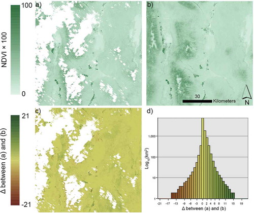
Often in GIS and remote sensing products, “no data” values are used to denote background areas, masked out areas, areas covered by clouds, or areas impacted by cloud shadows. Some data mining models can handle “no data” values, using non-numeric characters to flag no-data observations and input missing values (See5: An Informal Tutorial, 12/27/2017, http://rulequest.com/see5-win.html, An Overview of Cubist, 12/27/2017, http://rulequest.com/cubist-win.html). However, GIS and remotely sensed raster data are numerical data stored in spatial arrays. In GIS and remote sensing raster datasets, “no data” is often represented by a unique number like −999, 0, or something similar. Regression trees can be trained to recognize the “no data” associated numeric value as having no predictive value given adequate observations with “no data” values. This approach was used by Gu and Wylie (2015a) to cross different Landsat path/row boundaries seamlessly, and by (Boyte et al. 2017) to downscale from 250m to 30m using multiple date Landsat mosaics with some cloud contamination. We were able to seamlessly predict Landsat 8 Operational Land Imager (OLI) NDVI from temporally adjacent scenes of Landsat OLI and Sentinel Multispectral Instrument (MSI) using the Cubist regression tree “no data” value for clouds, snow, shadows, or water (Figure 3) (Pastick, Wylie, and Wu 2018). To aid in visual interpretation of Figure 3, the Great Basin areas with low modeled NDVI values are were clay playas or rocky/snow covered mountaintops occur and are nearly completely devoid of any vegetation. Helmer and Ruefenacht (2005) used regression trees to estimate Landsat reflectances in cloud contaminated scenes.

Figure 3. a) Normalized difference vegetation index (NDVI * 100) of Landsat 8 image acquired on 25 May 2016; b) NDVI synthetic Landsat image for 25 May 2106, generated with a regression tree model driven by Landsat OLI and Sentinel (MSI) time series data; c) Difference between real and synthetic images; and d) histogram of NDVI differences between real and synthetic images. Areas in white (no data) represent cloud, shadow, snow/ice, or water as identified from a decision tree masking model.

7. Approaches that did not work

We have seen that localized applications of regression and classification trees often capture more local detail (Zhang et al. 2010) vs (Boyte et al. 2018); (Pastick et al. 2013) vs (Pastick et al. 2015); (Boyte, Wylie, and Major 2015) vs (Boyte and Wylie 2017). One strategy we tested was constructing an overarching generalized descriptive model with a limited number of terminal predictive nodes, or rules, for regional mapping efforts. The predictive terminal nodes, or rules, of this overarching descriptive tree served as stratification, where subset models were then developed separately for each of the strata. This unpublished finding did not significantly improve carbon flux mapping accuracy in Wylie et al. (2016). In hindsight, this approach merely replicated the hierarchical structure already provided by a single overarching regression tree.

Another question we asked was once multiple versions of maps are produced with the regression tree approach, can the output ensemble maps then optimally be stratified and integrated to produce the best possible locally optimal combinations, or the best prediction, of the various map versions? Part of the logic here is that by combining multiple regression tree estimates in this manner, one may approximate or even improve on a random forest estimate. This approach was tried in Wylie et al. (2014) with several spatial variables added to aid with stratification for the multiple output integration model, but no significant improvement in accuracy was observed over each of the original mapped versions. This was probably related to the multiple regression tree outputs being highly correlated, unlike random forest ensemble predictions, which are not highly correlated (Cutler et al. 2007).

In some mapping applications, reference data is spatially exhaustive, as when developing multiple year crop type maps (Howard and Wylie 2014), multiple year ecosystem performance models (Wylie et al. 2014; Boyte, Wylie, and Major 2016), or downscaling MODIS NDVI (Gu and Wylie 2015b). This means that the predicted map can be differenced from the actual reference map to identify model residuals (e.g. Figure 3). Additional training points can then be added at “problematic” locations to ideally make the mapping algorithm pay more attention to these kinds of conditions (conceptually similar to a spatial variation of boosting). However, this approach has never appreciably improved accuracy and in some cases has decreased model accuracy. This implies that either 1) the spatial input variables are simply unable to explain this additional variation, or 2) too many noisy, mixed pixels (many were along the edges of water bodies), or erroneous pixels, were added to the model development database. With the increased incidence of noise or very difficult prediction cases, some of the prediction nodes or rules in the regression tree model could primarily be made up of the noisy or outlier pixels, and a more general (more severely pruned and less accurate) model would now be needed to better filter the noise into the error component of the prediction nodes.

8. Leveraging the power of parallel processing

The combination of data mining mapping with high performance computing and consistent remotely sensed data archives such as is available via Google Earth Engine^TM (Gorelick et al. 2017) and Amazon Web Services (https://aws.amazon.com/earth/, accessed on 18/04/2018) have opened doors for large-scale geospatial analysis and monitoring. For example, researchers have leveraged high performance computing platforms and data mining techniques to map global surface water change (Pekel et al. 2016), global forest change (Hansen et al. 2013), soil types in the United States (Padarian, Minasny, and McBratney 2015), rangeland indicators (McCord et al. 2017), and land cover (Giri et al. 2013). Unleashing the power of parallel processing facilitates timely processing of vast temporal and spatial databases such as the U.S. Landsat Analysis Ready Data (U.S. Landsat Analysis Ready Data, 12/27/17, https://landsat.usgs.gov/ard). The future possibility of data mining applications for mapping are thus greatly enhanced for longer time domains and larger spatial domains.

A number of machine learning classifiers (e.g., CART, Random Forest, SVM, ANNs) are available within the aforementioned cloud-computing platforms. Nevertheless, developing and applying complex machine learning models to large geospatial datasets is not trivial and may require leveraging multiple computing platforms or tools. For example, the computational model currently employed by Earth Engine performs poorly for recursion processes and operations that require a large amount of data to be cached at the same time, such as training many machine learning models (Gorelick et al. 2017). To circumvent such issues, users can train models at scale elsewhere in the Google Cloud Platform (Gonzalez and Krishnan 2015) and exploit Earth Engine for data management, pre-processing, image classification, post-processing, and visualization. Such tools make it easier for geospatial data scientists to apply machine learning techniques to their own big data problems and therefore greatly enhance our ability to monitor and manage the Earth’s landscapes and resources.

9. Conclusions

Data mining algorithms have advanced mapping accuracies by expanding beyond simple maximum likelihood predictions and regression modeling into nonlinear, non-parametric algorithms capable of integrating categorical and numerical data to optimize predictions. The major strengths of data mining approaches include an ability to deal with high order interactions and insensitivity to noise. Informed data mining analysis can mitigate overfitting tendencies, reduce prediction biases, and allow useful “no data” applications in complex mapping algorithms. Application of spatial data and remote sensing with data mining approaches for mapping has the potential to dramatically augment ecological spatio-temporal data stream quality and extent, furthering our understanding of complex natural systems.

Acknowledgements

This work was supported by the U.S. Geological Survey Land Change Science and Land Imaging Programs and the U.S. Geological Survey EROS Library. Additionally, this project was supported by the USGS Land Remote Sensing Program and the LANDFIRE Program. ASRC Federal InuTeq, LLC, contractor work was performed under USGS contract G13PC00028. Stinger Ghaffarian Technologies, Inc., contractor work was performed under USGS contract G08PC91508. Innovate!, Inc., contractor work performed under USGS contract G15PC00012. N.J.P. acknowledges additional funding support from the University of Minnesota’s (UMN) Doctoral Dissertation Fellowship. Any use of trade, firm or product names is for descriptive purposes only and does not imply endorsement by the US Government.

Disclosure statement

No potential conflict of interest was reported by the authors.

Additional information

Funding

This work was supported by the U.S. Geological Survey Land Change Science Program [USGS contract G15PC00012]; University of Minnesota’s (UMN) Doctoral Dissertation Fellowship; U.S. Geological Survey Land Change Science Prog [USGS contract G08PC91508]; USGS Land Remote Sensing Program and the LANDFIRE Program [USGS contract G08PC91508].

References

- Abadi, M., P. Barham, J. Chen, Z. Chen, A. Davis, J. Dean, M. Devin, S. Ghemawat, G. Irving, and M. Isard. 2016. "Tensorflow: A System for Large-Scale Machine Learning". In OSDI '16, Proceedings of the 12th USENIX Conference on Operating Systems Design and Implementation, 265–283. Berkeley, CA: USENIX Association.
- Abdel-Rahman, E. M., O. Mutanga, E. Adam, and R. Ismail. 2014. “Detecting Sirex Noctilio Grey-Attacked and Lightning-Struck Pine Trees Using Airborne Hyperspectral Data, Random Forest and Support Vector Machines Classifiers.” ISPRS Journal of Photogrammetry and Remote Sensing 88: 48–59. doi:10.1016/j.isprsjprs.2013.11.013.
- Adelabu, S., O. Mutanga, E. Adam, and M. A. Cho. 2013. “Exploiting Machine Learning Algorithms for Tree Species Classification in a Semiarid Woodland Using RapidEye Image.” Journal of Applied Remote Sensing 7 (1): article 073480. doi:10.1117/1.JRS.7.073480.
- Adeli, H., and A. Panakkat. 2009. “A Probabilistic Neural Network for Earthquake Magnitude Prediction.” Neural Networks: the Official Journal of the International Neural Network Society 22 (7): 1018–1024. doi:10.1016/j.neunet.2009.05.003.
- Alexander, C. 2008. Quantitative Methods in Finance. Hoboken, NJ: Wiley.
- Araújo, M. B., R. G. Pearson, W. Thuiller, and M. Erhard. 2005. “Validation of Species-Climate Impact Models under Climate Change.” Global Change Biology 11 (9): 1504–1513. doi:10.1111/j.1365-2486.2005.01000.x.
- Baker, C., R. Lawrence, C. Montagne, and D. Patten. 2006. “Mapping Wetlands and Riparian Areas Using Landsat ETM+ Imagery and Decision-Tree-Based Models.” Wetlands 26 (2): 465–474. doi:10.1672/0277-5212(2006)26[465:MWARAU]2.0.CO;2.
- Benitez, J. M., J. L. Castro, and I. Requena. 1997. “Are Artificial Neural Networks Black Boxes?” IEEE Transactions on Neural Networks 8 (5): 1156–1164. doi:10.1109/72.623216.
- Benning, A. 2012. “Spatial Cross-Validation and Bootstrap for the Assessment of Prediction Rules in Remote Sensing: The R Package Sperrorest.” In Proceedings of the 2012 IEEE International Geoscience and Remote Sensing Symposium, 5372–5375. Piscataway, NJ: Institute of Electrical and Electronics Engineers (IEEE). doi:10.1109/IGARSS.2012.6352393.
- Boyte, S. P., and B. K. Wylie. 2017. “Near-Real-Time Herbaceous Annual Cover in the Sagebrush Ecosystem (June 19, 2017).” In U.S. Geological Survey, ScienceBase. doi:10.5066/F7M32TNF.
- Boyte, S. P., B. K. Wylie, and D. J. Major. 2015. “Mapping and Monitoring Cheatgrass Dieoff in Rangelands of the Northern Great Basin, USA.” Rangeland Ecology & Management 68 (1): 18–28. doi:10.1016/j.rama.2014.12.005.
- Boyte, S. P., B. K. Wylie, and D. J. Major. 2016. “Cheatgrass Percent Cover Change: Comparing Recent Estimates to Climate Change−Driven Predictions in the Northern Great Basin.” Rangeland Ecology & Management 69 (4): 265–279. doi:10.1016/j.rama.2016.03.002.
- Boyte, S. P., B. K. Wylie, D. M. Howard, D. Dahal, and T. G. Gilmanov. 2018. “Estimating Carbon and Showing Impacts of Drought Using Satellite Data in Regression-Tree Models.” International Journal of Remote Sensing 39 (2): 374–398. doi:10.1080/01431161.2017.1384592.
- Boyte, S. P., B. K. Wylie, M. B. Rigge, and D. Dahal. 2017. “Fusing MODIS with Landsat 8 Data to Downscale Weekly Normalized Difference Vegetation Index Estimates for Central Great Basin Rangelands, USA.” GIScience & Remote Sensing. doi:10.1080/15481603.2017.1382065.
- Breiman, L., M. Last, and J. Rice. 2003. “Random Forests: Finding Quasars.” In: Statistical Challenges in Astronomy, edited by E. D. Feigelson and G. J. Babu, 243–254. New York: Springer. doi:10.1007/0-387-21529-8_16.
- Brown, J. F., B. D. Wardlow, T. Tadesse, M. J. Hayes, and B. C. Reed. 2008. “The Vegetation Drought Response Index (Vegdri): A New Integrated Approach for Monitoring Drought Stress in Vegetation.” GIScience & Remote Sensing 45 (1): 16–46. doi:10.2747/1548-1603.45.1.16.
- Brownlee, J. 2016. “Overfitting and Underfitting with Machine Learning Algorithms.” Machine Learning Algorithms. Accessed July 31, 2017. https://machinelearningmastery.com/overfitting-and-underfitting-with-machine-learning-algorithms/.
- Burrough, P. A., J. P. Wilson, P. F. M. van Gaans, and A. J. Hansen. 2001. “Fuzzy K-Means Classification of Topo-Climatic Data as an Aid to Forest Mapping in the Greater Yellowstone Area, USA.” Landscape Ecology 16 (6): 523–546. doi:10.1023/A:101316771.
- Castelluccio, M., G. Poggi, C. Sansone, and L. Verdoliva. 2015. “Land Use Classification in Remote Sensing Images by Convolutional Neural Networks.” arXiv preprint: arXiv:1605.01156. https://arxiv.org/abs/1508.00092
- Chaney, N. W., E. F. Wood, A. B. McBratney, J. W. Hempel, T. W. Nauman, C. W. Brungard, and N. P. Odgers. 2016. “POLARIS: A 30-Meter Probabilistic Soil Series Map of the Contiguous United States.” Geoderma 274: 54–67. doi:10.1016/j.geoderma.2016.03.025.
- Chen, T., and C. Guestrin. 2016. "Xgboost: A Scalable Tree Boosting System". In Proceedings of the ACM SIGKDD International Conference on Knowledge Discovery and Data Mining, 785–794. New York, NY: Association for Computing Machinery. doi:10.1145/2939672.
- Cieslak, D. A., and N. V. Chawla. 2008. “Learning Decision Trees for Unbalanced Data.” In: Machine Learning and Knowledge Discovery in Databases. ECML PKDD 2008. Lecture Notes in Computer Science, edited by W. Daelemans, B. Goethals, and K. Morik, Vol. 5211, 241–256. Berlin: Springer. https://dl.acm.org/citation.cfm?id=1431970.
- Congalton, R. G., and K. Green. 2008. Assessing The Accuracy Of Remotely Sensed Data: Principles and Practices. Boca Raton, FL: CRC Press.
- Cracknell, M. J., and A. M. Reading. 2014. “Geological Mapping Using Remote Sensing Data: A Comparison of Five Machine Learning Algorithms, Their Response to Variations in the Spatial Distribution of Training Data and the Use of Explicit Spatial Information.” Computers & Geosciences 63 (Suppl. C): 22–33. doi:10.1016/j.cageo.2013.10.008.
- Cutler, D. R., T. C. Edwards, K. H. Beard, A. Cutler, K. T. Hess, J. Gibson, and J. J. Lawler. 2007. “Random Forests for Classification in Ecology.” Ecology 88 (11): 2783–2792. doi:10.1890/07-0539.1.
- De Ville, B. 2006. Decision Trees for Business Intelligence and Data Mining: Using SAS Enterprise Miner. Cary, NC: SAS Institute.
- De’ath, G., and K. E. Fabricius. 2000. “Classification and Regression Trees: A Powerful yet Simple Technique for Ecological Data Analysis.” Ecology 81 (11): 3178–3192. doi:10.1890/0012-9658(2000)081[3178:CARTAP]2.0.CO;2.
- Debeljak, M., S. Džeroski, K. Jerina, A. Kobler, and M. Adamič. 2001. “Habitat Suitability Modelling for Red Deer (Cervus Elaphus L.) In South-Central Slovenia with Classification Trees.” Ecological Modelling 138 (1): 321–330. doi:10.1016/S0304-3800(00)00411-7.
- DeFries, R. S., and J. C.-W. Chan. 2000. “Multiple Criteria for Evaluating Machine Learning Algorithms for Land Cover Classification from Satellite Data.” Remote Sensing of Environment 74 (3): 503–515. doi:10.1016/S0034-4257(00)00142-5.
- Díaz-Uriarte, R., and S. Alvarez de Andrés. 2006. “Gene Selection and Classification of Microarray Data Using Random Forest.” BMC Bioinformatics 7 (1): 1–13. doi:10.1186/1471-2105-7-3.
- Dietterich, T. G. 2000. “An Experimental Comparison of Three Methods for Constructing Ensembles of Decision Trees: Bagging, Boosting, and Randomization.” Machine Learning 40 (2): 139–157. doi:10.1023/A:1007607513941.
- Du, J., Y. Liu, Y. Yu, and W. Yan. 2017. “A Prediction of Precipitation Data Based on Support Vector Machine and Particle Swarm Optimization (PSO-SVM) Algorithms.” Algorithms 10 (2): article 57. doi:10.3390/a10020057.
- Duda, R. O., P. E. Hart, and D. G. Stork. 2001. Pattern Classification. New York, NY: Wiley.
- Elith, J., J. R. Leathwick, and T. Hastie. 2008. “A Working Guide to Boosted Regression Trees.” Journal of Animal Ecology 77 (4): 802–813. doi:10.1111/j.1365-2656.2008.01390.x.
- Fan, W., and A. Bifet. 2012. “Mining Big Data: Current Status, and Forecast to the Future.” ACM SIGKDD Explorations Newsletter 14 (2): 1–5. doi:10.1145/2481244.2481246.
- Fassnacht, F. E., H. Latifi, A. Ghosh, P. K. Joshi, and B. Koch. 2014. “Assessing the Potential of Hyperspectral Imagery to Map Bark Beetle-Induced Tree Mortality.” Remote Sensing of Environment 140: 533–548. doi:10.1016/j.rse.2013.09.014.
- Fayyad, U., G. Piatetsky-Shapiro, and P. Smyth. 1996. “From Data Mining to Knowledge Discovery in Databases.” AI Magazine 17 (3): 37–54. doi:10.1609/aimag.v17i3.1230.
- Fernández-Delgado, M., E. Cernadas, S. Barro, and D. Amorim. 2014. “Do We Need Hundreds of Classifiers to Solve Real World Classification Problems?” Journal of Machine Learning Research 15: 3133–3181. http://www.jmlr.org/papers/volume15/delgado14a/delgado14a.pdf.
- Foody, G. M. 2004. “Thematic Map Comparison: Evaluating the Statistical Significance of Differences in Classification Accuracy.” Photogrammetric Engineering and Remote Sensing 70 (5): 627–633. doi:10.14358/PERS.70.5.627.
- Foody, G. M., and A. Mathur. 2004. “A Relative Evaluation of Multiclass Image Classification by Support Vector Machines.” IEEE Transactions on Geoscience and Remote Sensing 42 (6): 1335–1343. doi:10.1109/TGRS.2004.827257.
- Forkuor, G., O. K. L. Hounkpatin, G. Welp, and M. Thiel. 2017. “High Resolution Mapping of Soil Properties Using Remote Sensing Variables in South-Western Burkina Faso: A Comparison of Machine Learning and Multiple Linear Regression Models.” PLoS ONE 12 (1): e0170478. doi:10.1371/journal.pone.0170478.
- Fortmann-Roe, S. 2012. “Understanding the Bias-Variance Tradeoff.” Scott Fortmann-Roe: Model Architect & Software Developer. Accessed 31 July 2017. http://scott.fortmann-roe.com/docs/BiasVariance.html.
- Friedl, M. A., and C. E. Brodley. 1997. “Decision Tree Classification of Land Cover from Remotely Sensed Data.” Remote Sensing of Environment 61 (3): 399–409. doi:10.1016/S0034-4257(97)00049-7.
- Friedl, M. A., C. E. Brodley, and A. H. Strahler. 1999. “Maximizing Land Cover Classification Accuracies Produced by Decision Trees at Continental to Global Scales.” IEEE Transactions on Geoscience and Remote Sensing 37 (2): 969–977. doi:10.1109/36.752215.
- Friedl, M. A., D. Sulla-Menashe, B. Tan, A. Schneider, N. Ramankutty, A. Sibley, and X. Huang. 2010. “MODIS Collection 5 Global Land Cover: Algorithm Refinements and Characterization of New Datasets.” Remote Sensing of Environment 114 (1): 168–182. doi:10.1016/j.rse.2009.08.016.
- Furlanello, C., M. Neteler, S. Merler, S. Menegon, S. Fontanari, A. Donini, A. Rizzoli, and C. Chemini. 2003. “GIS and the Random Forest Predictor: Integration in R for Tick-Borne Disease Risk Assessment.” In Proceedings of the 3rd International Workshop on Distributed Statistical Computing (DSC 2003). edited by K. Hornik, F. Leisch, and A. Zeileis, 1–11. Vienna: Austrian Association for Statistical Computing (AASC) and the R Foundation for Statistical Computing. https://www.r-project.org/conferences/DSC-2003/Proceedings/
- Ghimire, B., J. Rogan, V. Galiano, P. Panday, and N. Neeti. 2012. “An Evaluation of Bagging, Boosting, and Random Forests for Land-Cover Classification in Cape Cod, Massachusetts, USA.” GIScience and Remote Sensing 49 (5): 623–643. doi:10.2747/1548-1603.49.5.623.
- Giambelluca, T. W., Q. Chen, A. G. Frazier, J. P. Price, Y.-L. Chen, P.-S. Chu, J. K. Eischeid, and D. M. Delparte. 2012. “Online Rainfall Atlas of Hawai‘I.” Bulletin of the American Meteorological Society 94 (3): 313–316. doi:10.1175/BAMS-D-11-00228.1.
- Giri, C., B. Pengra, J. Long, and T. R. Loveland. 2013. “Next Generation of Global Land Cover Characterization, Mapping, and Monitoring.” International Journal of Applied Earth Observation and Geoinformation 25: 30–37. doi:10.1016/j.jag.2013.03.005.
- Gleason, C. J., and J. Im. 2012. “Forest Biomass Estimation from Airborne LiDAR Data Using Machine Learning Approaches.” Remote Sensing of Environment 125 (Suppl. C): 80–91. doi:10.1016/j.rse.2012.07.006.
- Gómez-Chova, L., G. Camps-Valls, J. Muñoz-Mari, and J. Calpe. 2008. “Semisupervised Image Classification with Laplacian Support Vector Machines.” IEEE Geoscience and Remote Sensing Letters 5 (3): 336–340. doi:10.1109/LGRS.2008.916070.
- Gonzalez, J. U., and S. P. T. Krishnan. 2015. Building Your Next Big Thing with Google Cloud Platform: A Guide for Developers and Enterprise Architects. Berkeley, CA: Apress.
- Gorelick, N., M. Hancher, M. Dixon, S. Ilyushchenko, D. Thau, and R. Moore. 2017. “Google Earth Engine: Planetary-Scale Geospatial Analysis for Everyone.” Remote Sensing of Environment 202: 18–28. doi:10.1016/j.rse.2017.06.031.
- Goswami, S., S. Chakraborty, S. Ghosh, A. Chakrabarti, and B. Chakraborty. 2016. “A Review on Application of Data Mining Techniques to Combat Natural Disasters.” Ain Shams Engineering Journal. doi: 10.1016/j.asej.2016.01.012.
- Gu, Y., and B. K. Wylie. 2015a. “Developing a 30-M Grassland Productivity Estimation Map for Central Nebraska Using 250-M MODIS and 30-M Landsat-8 Observations.” Remote Sensing of Environment 171: 291–298. doi:10.1016/j.rse.2015.10.018.
- Gu, Y., and B. K. Wylie. 2015b. “Downscaling 250-M MODIS Growing Season NDVI Based on Multiple-Date Landsat Images and Data Mining Approaches.” Remote Sensing 7 (4): 3489–3506. doi:10.3390/rs70403489.
- Gu, Y., B. K. Wylie, S. P. Boyte, J. J. Picotte, D. M. Howard, K. Smith, and K. J. Nelson. 2016. “An Optimal Sample Data Usage Strategy to Minimize Overfitting and Underfitting Effects in Regression Tree Models Based on Remotely-Sensed Data.” Remote Sensing 8 (11): 1–13. doi:10.3390/rs8110943.
- Gu, Y., D. M. Howard, B. K. Wylie, and L. Zhang. 2012. “Mapping Carbon Flux Uncertainty and Selecting Optimal Locations for Future Flux Towers in the Great Plains.” Landscape Ecology 27 (3): 319–326. doi:10.1007/s10980-011-9699-7.
- Han, L., J. Sun, W. Zhang, Y. Xiu, H. Feng, and Y. Lin. 2017. “A Machine Learning Nowcasting Method Based on Real-Time Reanalysis Data.” Journal of Geophysical Research 122 (7): 4038–4051. doi:10.1002/2016JD025783.
- Hansen, M. C., P. V. Potapov, R. Moore, M. Hancher, S. A. Turubanova, A. Tyukavina, D. Thau, et al. 2013. “High-Resolution Global Maps of 21st-Century Forest Cover Change.” Science 342 (6160): 850–853. doi:10.1126/science.1244693.
- Hansen, M. C., R. Dubayah, and R. Defries. 1996. “Classification Trees: An Alternative to Traditional Land Cover Classifiers.” International Journal of Remote Sensing 17 (5): 1075–1081. doi:10.1080/01431169608949069.
- Hansen, M. C., R. S. DeFries, J. R. G. Townshend, M. Carroll, C. Dimiceli, and R. A. Sohlberg. 2003. “Global Percent Tree Cover at a Spatial Resolution of 500 Meters: First Results of the MODIS Vegetation Continuous Fields Algorithm.” Earth Interactions 7 (10): 1–15. doi:10.1175/1087-3562(2003)007<0001:GPTCAA>2.0.CO;2.
- Hastie, T., R. Tibshirani, and J. Friedman. 2009. The Elements of Statistical Learning: Data Mining, Inference, and Prediction. New York: Springer. doi:10.1007/978-0-387-84858-7.
- Hayes, T., S. Usami, R. Jacobucci, and J. J. McArdle. 2015. “Using Classification and Regression Trees (CART) and Random Forests to Analyze Attrition: Results from Two Simulations.” Psychology and Aging 30 (4): 911–929. doi:10.1037/pag0000046.
- Helmer, E. H., and B. Ruefenacht. 2005. “Cloud-Free Satellite Image Mosaics with Regression Trees and Histogram Matching.” Photogrammetric Engineering & Remote Sensing 71 (9): 1079–1089. doi:10.14358/PERS.71.9.1079.
- Henderson, B. L., E. N. Bui, C. J. Moran, and D. A. P. Simon. 2005. “Australia-Wide Predictions of Soil Properties Using Decision Trees.” Geoderma 124 (3): 383–398. doi:10.1016/j.geoderma.2004.06.007.
- Homer, C. G., C. Huang, L. Yang, B. K. Wylie, and M. Coan. 2004. “Development of a 2001 National Land-Cover Database for the United States.” Photogrammetric Engineering & Remote Sensing 7 (7): 829–840. doi:10.14358/PERS.70.7.829.
- Homer, C. G., D. K. Meyer, C. L. Aldridge, and S. J. Schell. 2013. “Detecting Annual and Seasonal Changes in a Sagebrush Ecosystem with Remote Sensing-Derived Continuous Fields.” Journal of Applied Remote Sensing 7 (1): 1–19. doi:10.1117/1.JRS.7.073508.
- Howard, D. M., and B. K. Wylie. 2014. “Annual Crop Type Classification of the U.S. Great Plains for 2000 to 2011.” Photogrammetric Engineering & Remote Sensing 80 (6): 537–549. doi:10.14358/PERS.80.6.537-549.
- Huang, C., L. Yang, B. K. Wylie, and C. G. Homer. 2001. “A Strategy for Estimating Tree Canopy Density Using Landsat 7 ETM+ and High Resolution Images over Large Areas.” In: Proceedings of the 3rd International Conference on Geospatial Information in Agriculture and Forestry, 1–9. Ann Arbor, MI: Veridian. http://landcover.usgs.gov/pdf/canopy_density.pdf.
- Huang, C., L. S. Davis, and J. R. G. Townshend. 2002. “An Assessment of Support Vector Machines for Land Cover Classification.” International Journal of Remote Sensing 23 (4): 725–749. doi:10.1080/01431160110040323.
- Jensen, J. R. 1996. Introductory Digital Image Processing: A Remote Sensing Perspective. 2nd Ed. Upper Saddle River, NJ: Prentice Hall.
- Jensen, J. R. 2016. Introductory Digital Image Processing: A Remote Sensing Perspective. 4th ed. Glenview, IL: Pearson Education.
- Kobler, A., and M. Adamic. 2000. “Identifying Brown Bear Habitat by a Combined GIS and Machine Learning Method.” Ecological Modelling 135 (2–3): 291–300. doi:10.1016/S0304-3800(00)00384-7.
- Kohavi, R. 1995. “A Study of Cross-Validation and Bootstrap for Accuracy Estimation and Model Selection.” In: Proceedings of the Fourteenth International Joint Conference on Artificial Intelligence (IJCAI), Vol. 2, 1137–1143. San Mateo, CA: Morgan Kaufman. https://www.ijcai.org/Proceedings/95-2/Papers/016.pdf
- Krahwinkler, P. M. 2013. “Machine Learning Based Classification for Semantic World Modeling: Support Vector Machine Based Decision Tree for Single Tree Level Forest Species Mapping.” PhD diss., RWTH Aaachen University. http://publications.rwth-aachen.de/record/229488?ln=de
- Lawrence, R. L., and A. Wright. 2001. “Rule-Based Classification Systems Using Classification and Regression Tree (CART) Analysis.” Photogrammetric Engineering & Remote Sensing 67 (10): 1137–1142. https://www.asprs.org/wp-content/uploads/pers/2001journal/october/2001_oct_1137-1142.pdf.
- Lawrence, R. L., S. D. Wood, and R. L. Sheley. 2006. “Mapping Invasive Plants Using Hyperspectral Imagery and Breiman Cutler Classifications (Randomforest).” Remote Sensing of Environment 100 (3): 356–362. doi:10.1016/j.rse.2005.10.014.
- Lee, B. K., J. Lessler, and E. A. Stuart. 2010. “Improving Propensity Score Weighting Using Machine Learning.” Statistics in Medicine 29 (3): 337–346. doi:10.1002/sim.3782.
- Li, M., J. Im, and C. Beier. 2013. “Machine Learning Approaches for Forest Classification and Change Analysis Using Multi-Temporal Landsat TM Images over Huntington Wildlife Forest.” GIScience and Remote Sensing 50 (4): 361–384. doi:10.1080/15481603.2013.819161.
- Lin, H. T., C. J. Lin, and R. C. Weng. 2007. “A Note on Platt’s Probabilistic Outputs for Support Vector Machines.” Machine Learning 68 (3): 267–276. doi:10.1007/s10994-007-5018-6.
- Liu, T., A. Abd-Elrahman, J. Morton, and V. L. Wilhelm. 2018. “Comparing Fully Convolutional Networks, Random Forest, Support Vector Machine, and Patch-Based Deep Convolutional Neural Networks for Object-Based Wetland Mapping Using Images from Small Unmanned Aircraft System.” GIScience and Remote Sensing 55 (2): 243–264. doi:10.1080/15481603.2018.1426091.
- Liu, W., S. Gopal, and C. E. Woodcock. 2004. “Uncertainty and Confidence in Land Cover Classification Using a Hybrid Classifier Approach.” Photogrammetric Engineering & Remote Sensing 70 (8): 963–971. doi:10.14358/PERS.70.8.963.
- Liu, Y., E. Racah, J. Correa, A. Khosrowshahi, D. Lavers, K. Kunkel, M. Wehner, and W. Collins. 2016. “Application of Deep Convolutional Neural Networks for Detecting Extreme Weather in Climate Datasets.” arXiv preprint: arXiv:1605.01156. https://arxiv.org/abs/1605.01156
- Liu, Y., and L. Wu. 2016. “Geological Disaster Recognition on Optical Remote Sensing Images Using Deep Learning.” Procedia Computer Science 91: 566–575. doi:10.1016/j.procs.2016.07.144.
- Loh, W.-Y. 2002. “Regression Trees with Unbiased Variable Selection and Interaction Detection.” Statistica Sinica 12 (2): 361–386. http://www.jstor.org/stable/24306967.
- Lyu, Z., G. Helene, Y. He, Q. Zhuang, A. D. McGuire, A. Bennett, A. L. Breen, et al. 2017. “The Role of Driving Factors in Historical and Projected Carbon Dynamics in Wetland Ecosystems of Alaska.” Paper presented at the Fall Meeting, American Geophysical Union, New Orleans, LA, December 11–15. https://agu.confex.com/agu/fm17/preliminaryview.cgi/Paper276021.html
- Maggiori, E., Y. Tarabalka, G. Charpiat, and P. Alliez. 2017. “Convolutional Neural Networks for Large-Scale Remote-Sensing Image Classification.” IEEE Transactions on Geoscience and Remote Sensing 55 (2): 645–657. doi:10.1109/TGRS.2016.2612821.
- Maingi, J. K., and W. M. Luhn. 2005. “Mapping Insect-Induced Pine Mortality in the Daniel Boone National Forest, Kentucky Using Landsat TM and ETM+ Data.” GIScience and Remote Sensing 42 (3): 224–250. doi:10.2747/1548-1603.42.3.224.
- McBratney, A. G., M. L. Mendonça Santos, and B. Minasny. 2003. “On Digital Soil Mapping.” Geoderma 117 (1–2): 3–52. doi:10.1016/S0016-7061(03)00223-4.
- McCord, S. E., M. Buenemann, J. W. Karl, D. M. Browning, and B. C. Hadley. 2017. “Integrating Remotely Sensed Imagery and Existing Multiscale Field Data to Derive Rangeland Indicators: Application of Bayesian Additive Regression Trees.” Rangeland Ecology & Management 70 (5): 644–655. doi:10.1016/j.rama.2017.02.004.
- McIver, D. K., and M. A. Friedl. 2001. “Estimating Pixel-Scale Land Cover Classification Confidence Using Nonparametric Machine Learning Methods.” IEEE Transactions on Geoscience and Remote Sensing 39 (9): 1959–1968. doi:10.1109/36.951086.
- Memarian, H., and S. K. Balasundram. 2012. “Comparison between Multi-Layer Perceptron and Radial Basis Function Networks for Sediment Load Estimation in a Tropical Watershed.” Journal of Water Resource and Protection 4: 870–876. doi:10.4236/jwarp.2012.410102.
- Miao, X., and J. S. Heaton. 2010. “A Comparison of Random Forest and Adaboost Tree in Ecosystem Classification in East Mojave Desert.” In 2010 18th International Conference on Geoinformatics, edited by Y. Liu and A. Chen, 1–6. Piscataway, NJ: Institute of Electrical and Electronics Engineers (IEEE). doi:10.1109/GEOINFORMATICS.2010.5567504.
- Michaelsen, J., D. S. Schimel, M. A. Friedl, F. W. Davis, and R. C. Dubayah. 1994. “Regression Tree Analysis of Satellite and Terrain Data to Guide Vegetation Sampling and Surveys.” Journal of Vegetation Science 5 (5): 673–686. doi:10.2307/3235882.
- Moisen, G. G., and T. S. Frescino. 2002. “Comparing Five Modelling Techniques for Predicting Forest Characteristics.” Ecological Modelling 157 (2–3): 209–225. doi:10.1016/S0304-3800(02)00197-7.
- Mountrakis, G., J. Im, and C. Ogole. 2011. “Support Vector Machines in Remote Sensing: A Review.” ISPRS Journal of Photogrammetry and Remote Sensing 66 (3): 247–259. doi:10.1016/j.isprsjprs.2010.11.001.
- Munther, A., A. Alalousi, S. Mizam, R. R. Othman, and M. Anbar. 2014. “Network Traffic Classification—A Comparative Study of Two Common Decision Tree Methods: C4.5 And Random Forest.” In: 2014 2nd International Conference on Electronic Design (ICED), 210–214. Piscataway, NJ: Institute of Electrical and Electronics Engineers (IEEE). doi:10.1109/ICED.2014.7015800.
- Mutanga, O., E. Adam, and M. A. Cho. 2012. “High Density Biomass Estimation for Wetland Vegetation Using WorldView-2 Imagery and Random Forest Regression Algorithm.” International Journal of Applied Earth Observation and Geoinformation 18: 399–406. doi:10.1016/j.jag.2012.03.012.
- National Land Cover Database 2011 (Product Data Downloads; accessed December 17, 2017). https://www.mrlc.gov/nlcd11_data.php.
- NASA. 2010. Measurement Uncertainty Analysis Principles and Methods—NASA Measurement Quality Assurance Handbook - ANNEX 3, NASA-HDBK-8739.19-3. Washington, DC: National Aeronautics and Space Administration. https://standards.nasa.gov/standard/nasa/nasa-hdbk-873919-3.
- Nauman, T. W., M. C. Duniway, M. L. Villarreal, and T. B. Poitras. 2017. “Disturbance Automated Reference Toolset (DART): Assessing Patterns in Ecological Recovery from Energy Development on the Colorado Plateau.” Science of the Total Environment 584-585: 476–488. doi:10.1016/j.scitotenv.2017.01.034.
- Nitze, I., U. Schulthess, and H. Asche. 2012. “Comparison of Machine Learning Algorithms Random Forest, Artificial Neural Network and Support Vector Machine to Maximum Likelihood for Supervised Crop Type Classification.” In: Proceedings of the 4th Conference on Geographic Object-Based Image Analysis - GEOBIA, 7–9. São José dos Campos, Brazil: Instituto Nacional de Pesquisas Espaciais - INPE. http://mtc-m16c.sid.inpe.br/col/sid.inpe.br/mtc-m18/2012/05.15.13.21/doc/015.pdf.
- Nourani, V., A. H. Baghanam, J. Adamowski, and M. Gebremichael. 2013. “Using Self-Organizing Maps and Wavelet Transforms for Space–Time Pre-Processing of Satellite Precipitation and Runoff Data in Neural Network Based Rainfall–Runoff Modeling.” Journal of Hydrology 476: 228–243. doi:10.1016/j.jhydrol.2012.10.054.
- Padarian, J., B. Minasny, and A. B. McBratney. 2015. “Using Google’s Cloud-Based Platform for Digital Soil Mapping.” Computers & Geosciences 83: 80–88. doi:10.1016/j.cageo.2015.06.023.
- Pal, M., and P. M. Mather. 2003. “An Assessment of the Effectiveness of Decision Tree Methods for Land Cover Classification.” Remote Sensing of Environment 86 (4): 554–565. doi:10.1016/S0034-4257(03)00132-9.
- Pal, M., and P. M. Mather. 2004. “Assessment of the Effectiveness of Support Vector Machines for Hyperspectral Data.” Future Generation Computer Systems 20 (7): 1215–1225. doi:10.1016/j.future.2003.11.011.
- Papale, D., and R. Valentini. 2003. “A New Assessment of European Forests Carbon Exchanges by Eddy Fluxes and Artificial Neural Network Spatialization.” Global Change Biology 9 (4): 525–535. doi:10.1046/j.1365-2486.2003.00609.x.
- Paruelo, J., and F. Tomasel. 1997. “Prediction of Functional Characteristics of Ecosystems: A Comparison of Artificial Neural Networks and Regression Models.” Ecological Modelling 98 (2): 173–186. doi:10.1016/S0304-3800(96)01913-8.
- Pastick, N. J., B. K. Wylie, and Z. Wu. 2018. “Spatiotemporal Analysis of Landsat and Sentinel Data to Support Monitoring of Dryland Ecosystems.” Remote Sensing. 10 (5) 791 doi:10.3390/rs10050791
- Pastick, N. J., M. Rigge, B. K. Wylie, M. T. Jorgenson, J. R. Rose, K. D. Johnson, and L. Ji. 2014. “Distribution and Landscape Controls of Organic Layer Thickness and Carbon within the Alaskan Yukon River Basin.” Geoderma 230-231 (Suppl. C): 79–94. doi:10.1016/j.geoderma.2014.04.008.
- Pastick, N. J., M. T. Jorgenson, B. K. Wylie, B. J. Minsley, L. Ji, M. A. Walvoord, B. D. Smith, J. D. Abraham, and J. R. Rose. 2013. “Extending Airborne Electromagnetic Surveys for Regional Active Layer and Permafrost Mapping with Remote Sensing and Ancillary Data, Yukon Flats Ecoregion, Central Alaska.” Permafrost and Periglacial Processes 24 (3): 184–199. doi:10.1002/ppp.1775.
- Pastick, N. J., M. T. Jorgenson, B. K. Wylie, S. J. Nield, K. D. Johnson, and A. O. Finley. 2015. “Distribution of Near-Surface Permafrost in Alaska: Estimates of Present and Future Conditions.” Remote Sensing of Environment 168: 301–315. doi:10.1016/j.rse.2015.07.019.
- Pedregosa, F., G. Varoquaux, A. Gramfort, V. Michel, B. Thirion, O. Grisel, and M. Blondel, et al. 2011. "Scikit-Learn: Machine Learning in Python". Journal of Machine Learning Research 12: 2825–2830. http://www.jmlr.org/papers/v12/pedregosa11a.ht
- Pekel, J.-F., A. Cottam, N. Gorelick, and A. S. Belward. 2016. “High-Resolution Mapping of Global Surface Water and Its Long-Term Changes.” Nature 540: 418–422. doi:10.1038/nature20584.
- Prasad, A. M., L. R. Iverson, and A. Liaw. 2006. “Newer Classification and Regression Tree Techniques: Bagging and Random Forests for Ecological Prediction.” Ecosystems 9 (2): 181–199. doi:10.1007/s10021-005-0054-1.
- Prince, S. D., and M. K. Steininger. 1999. “Biophysical Stratification of the Amazon Basin.” Global Change Biology 5 (1): 1–22. doi:10.1046/j.1365-2486.1998.00220.x.
- Razi, M. A., and K. Athappilly. 2005. “A Comparative Predictive Analysis of Neural Networks (Nns), Nonlinear Regression and Classification and Regression Tree (CART) Models.” Expert Systems with Applications 29 (1): 65–74. doi:10.1016/j.eswa.2005.01.006.
- Rodriguez-Galiano, V. F., B. Ghimire, J. Rogan, M. Chica-Olmo, and J. P. Rigol-Sanchez. 2012. “An Assessment of the Effectiveness of a Random Forest Classifier for Land-Cover Classification.” ISPRS Journal of Photogrammetry and Remote Sensing 67 (Suppl. C): 93–104. doi:10.1016/j.isprsjprs.2011.11.002.
- Romero, A., C. Gatta, and G. Camps-Valls. 2016. “Unsupervised Deep Feature Extraction for Remote Sensing Image Classification.” IEEE Transactions on Geoscience and Remote Sensing 54 (3): 1349–1362. doi:10.1109/TGRS.2015.2478379.
- Rover, J., B. K. Wylie, and L. Ji. 2010. “A Self-Trained Classification Technique for Producing 30 M Percent-Water Maps from Landsat Data.” International Journal of Remote Sensing 31 (8): 2197–2203. doi:10.1080/01431161003667455.
- Rupp, T. S., M. Olson, L. G. Adams, B. W. Dale, K. Joly, J. Henkelman, W. B. Collins, and A. M. Starfield. 2006. “Simulating the Influences of Various Fire Regimes on Caribou Winter Habitat.” Ecological Applications 16 (5): 1730–1743. doi:10.1890/1051-0761(2006)016[1730:STIOVF]2.0.CO;2.
- Schwabacher, M., and P. Langley. 2001. “Discovering Communicable Scientific Knowledge from Spatio-Temporal Data.” In: Proceedings of the 18th International Conference on Machine Learning. edited by C. E. Brodley, 489–496. San Francisco, CA: Morgan Kaufmann. https://ntrs.nasa.gov/search.jsp?R=20010087029
- Singh, N., L-M.. Browne, and R. Butler. 2013. “Parallel Astronomical Data Processing with Python: Recipes for Multicore Machines.” Recipes for Multicore Machines". Astronomy and Computing 2: 1–10. doi: 10.1016/j.ascom.2013.04.002.
- Sohl, T., and K. Sayler. 2008. “Using the FORE-SCE Model to Project Land-Cover Change in the Southeastern United States.” Ecological Modelling 219 (1): 49–65. doi:10.1016/j.ecolmodel.2008.08.003.
- Srivastava, N., G. Hinton, A. Krizhevsky, I. Sutskever, and R. Salakhutdinov. 2014. “Dropout: A Simple Way to Prevent Neural Networks from Overfitting.” Journal of Machine Learning Research 15: 1929–1958. http://www.jmlr.org/papers/v15/srivastava14a.html.
- Steyerberg, E. W., S. E. Bleeker, H. A. Moll, D. E. Grobbee, and K. G. M. Moons. 2003. “Internal and External Validation of Predictive Models: A Simulation Study of Bias and Precision in Small Samples.” Journal of Clinical Epidemiology 56 (5): 441–447. doi:10.1016/S0895-4356(03)00047-7.
- Strobl, C., J. Malley, and G. Tutz. 2009. “An Introduction to Recursive Partitioning: Rationale, Application and Characteristics of Classification and Regression Trees, Bagging and Random Forests.” Psychological Methods 14 (4): 323–348. doi:10.1037/a0016973.
- Sutton, C. D. 2005. “Classification and Regression Trees, Bagging, and Boosting.” In Chap. 11 in Handbook of Statistics, edited by C. R. Rao, E. J. Wegman, and J. L. Solka, Vol. 24. Amsterdam: Elsevier. doi:10.1016/S0169-7161(04)24011-1.
- Tadesse, T., C. Champagne, B. D. Wardlow, T. A. Hadwen, J. F. Brown, G. B. Demisse, Y. A. Bayissa, and A. M. Davidson. 2017. “Building the Vegetation Drought Response Index for Canada (Vegdri-Canada) to Monitor Agricultural Drought: First Results.” GIScience and Remote Sensing 54 (2): 230–257. doi:10.1080/15481603.2017.1286728.
- Tehrany, M. S., B. Pradhan, and M. N. Jebur. 2014. “Flood Susceptibility Mapping Using a Novel Ensemble Weights-of-Evidence and Support Vector Machine Models in GIS.” Journal of Hydrology 512: 332–343. doi:10.1016/j.jhydrol.2014.03.008.
- Tesfamichael, S. G., S. W. Newete, E. Adam, and B. Dubula. 2018. “Field Spectroradiometer and Simulated Multispectral Bands for Discriminating Invasive Species from Morphologically Similar Cohabitant Plants.” GIScience and Remote Sensing 55 (3): 417–436. doi:10.1080/15481603.2017.1396658.
- Tittonell, P., K. D. Shepherd, B. Vanlauwe, and K. E. Giller. 2008. “Unravelling the Effects of Soil and Crop Management on Maize Productivity in Smallholder Agricultural Systems of Western Kenya—An Application of Classification and Regression Tree Analysis.” Agriculture, Ecosystems & Environment 123 (1): 137–150. doi:10.1016/j.agee.2007.05.005.
- Torbick, N., and M. Corbiere. 2015. “Mapping Urban Sprawl and Impervious Surfaces in the Northeast United States for the past Four Decades.” GIScience and Remote Sensing 52 (6): 746–764. doi:10.1080/15481603.2015.1076561.
- Tso, B., and P. Mather. 2009. Classification Methods for Remotely Sensed Data. Boca Raton, FL: CRC Press.
- Tu, J. V. 1996. “Advantages and Disadvantages of Using Artificial Neural Networks versus Logistic Regression for Predicting Medical Outcomes.” Journal of Clinical Epidemiology 49 (11): 1225–1231. doi:10.1016/S0895-4356(96)00002-9.
- Utz, H. F., A. E. Melchinger, and C. C. Schön. 2000. “Bias and Sampling Error of the Estimated Proportion of Genotypic Variance Explained by Quantitative Trait Loci Determined from Experimental Data in Maize Using Cross Validation and Validation with Independent Samples.” Genetics 154 (4): 1839–1849. http://www.genetics.org/content/genetics/154/4/1839.full.pdf.
- Vapnik, V. 1995. The Nature of Statistical Learning Theory. New York: Springer-Verlag.
- Verbyla, D. L., and J. A. Litvaitis. 1989. “Resampling Methods for Evaluating Classification Accuracy of Wildlife Habitat Models.” Environmental Management 13 (6): 783–787. doi:10.1007/BF01868317.
- Warmerdam, F. 2008. "The Geospatial Data Abstraction Library". In Open Source Approaches in Spatial Data Handling, edited by G.B. Hall and M.G. Leahy, 87–104. Berlin: Springer. doi:10.1007/978-3-540-74831-1_5.
- Warner, B., and M. Misra. 1996. “Understanding Neural Networks as Statistical Tools.” The American Statistician 50 (4): 284–293. doi:10.1080/00031305.1996.10473554.
- Weiss, G. M., and F. Provost. 2003. “Learning When Training Data are Costly: The Effect of Class Distribution on Tree Induction.” Journal of Artificial Intelligence Research 19: 315–354. doi:10.1613/jair.1199.
- Wickham, J. D., S. V. Stehman, L. Gass, J. Dewitz, J. A. Fry, and T. G. Wade. 2013. “Accuracy Assessment of NLCD 2006 Land Cover and Impervious Surface.” Remote Sensing of Environment 130: 294–304. doi:10.1016/j.rse.2012.12.001.
- Wu, X., V. Kumar, J. R. Quinlan, J. Ghosh, Q. Yang, H. Motoda, G. J. McLachlan, et al. 2008. “Top 10 Algorithms in Data Mining.” Knowledge and Information Systems 14 (1): 1–37. doi:10.1007/s10115-007-0114-2.
- Wylie, B., M. Rigge, B. Brisco, K. Murnaghan, J. Rover, and J. Long. 2014. “Effects of Disturbance and Climate Change on Ecosystem Performance in the Yukon River Basin Boreal Forest.” Remote Sensing 6 (10): 9145–9169. doi:10.3390/rs6109145.
- Wylie, B. K., D. A. Johnson, E. Laca, N. Z. Saliendra, T. G. Gilmanov, B. C. Reed, L. L. Tieszen, and B. B. Worstell. 2003. “Calibration of Remotely Sensed, Coarse Resolution NDVI to CO2 Fluxes in a Sagebrush-Steppe Ecosystem.” Remote Sensing of Environment 85 (2): 243–255. doi:10.1016/S0034-4257(03)00004-X.
- Wylie, B. K., D. M. Howard, D. Dahal, T. Gilmanov, L. Ji, L. Zhang, and K. Smith. 2016. “Grassland and Cropland Net Ecosystem Production of the U.S. Great Plains: Regression Tree Model Development and Comparative Analysis.” Remote Sensing 8 (11): 944. doi:10.3390/rs8110944.
- Wylie, B. K., E. A. Fosnight, T. G. Gilmanov, A. B. Frank, J. A. Morgan, M. R. Haferkamp, and T. P. Meyers. 2007. “Adaptive Data-Driven Models for Estimating Carbon Fluxes in the Northern Great Plains.” Remote Sensing of Environment 106 (4): 399–413. doi:10.1016/j.rse.2006.09.017.
- Wylie, B. K., L. Zhang, N. Bliss, L. Ji, L. L. Tieszen, and W. M. Jolly. 2008. “Integrating Modelling and Remote Sensing to Identify Ecosystem Performance Anomalies in the Boreal Forest, Yukon River Basin, Alaska.” International Journal of Digital Earth 1 (2): 196–220. doi:10.1080/17538940802038366.
- Xiao, J., Q. Zhuang, D. D. Baldocchi, B. E. Law, A. D. Richardson, J. Chen, R. Oren, et al. 2008. “Estimation of Net Ecosystem Carbon Exchange for the Conterminous United States by Combining MODIS and AmeriFlux Data.” Agricultural and Forest Meteorology 148 (11): 1827–1847. doi:10.1016/j.agrformet.2008.06.015.
- Yang, L., C. Huang, C. G. Homer, B. K. Wylie, and M. J. Coan. 2003. “An Approach for Mapping Large-Area Impervious Surfaces: Synergistic Use of Landsat-7 ETM+ and High Spatial Resolution Imagery.” Canadian Journal of Remote Sensing 29 (2): 230–240. doi:10.5589/m02-098.
- Yilmaz, K. K., T. S. Hogue, K.-L. Hsu, S. Sorooshian, H. V. Gupta, and T. Wagener. 2005. “Intercomparison of Rain Gauge, Radar, and Satellite-Based Precipitation Estimates with Emphasis on Hydrologic Forecasting.” Journal of Hydrometeorology 6 (4): 497–517. doi:10.1175/JHM431.1.
- Zare, M., H. R. Pourghasemi, M. Vafakhah, and B. Pradhan. 2013. “Landslide Susceptibility Mapping at Vaz Watershed (Iran) Using an Artificial Neural Network Model: A Comparison between Multilayer Perceptron (MLP) and Radial Basic Function (RBF) Algorithms.” Arabian Journal of Geosciences 6 (8): 2873–2888. doi:10.1007/s12517-012-0610-x.
- Zhang, L., B. K. Wylie, L. Ji, T. G. Gilmanov, and L. L. Tieszen. 2010. “Climate-Driven Interannual Variability in Net Ecosystem Exchange in the Northern Great Plains Grasslands.” Rangeland Ecology & Management 63 (1): 40–50. doi:10.2111/08-232.1.
- Zhu, X. X., D. Tuia, L. Mou, G. S. Xia, L. Zhang, F. Xu, and F. Fraundorfer. 2017. “Deep Learning in Remote Sensing: A Comprehensive Review and List of Resources.” IEEE Geoscience and Remote Sensing Magazine 5 (4): 8–36. doi:10.1109/MGRS.2017.2762307.
- Zhu, Z., A. L. Gallant, C. E. Woodcock, B. Pengra, P. Olofsson, T. R. Loveland, S. Jin, D. Dahal, L. Yang, and R. F. Auch. 2016. “Optimizing Selection of Training and Auxiliary Data for Operational Land Cover Classification for the LCMAP Initiative.” ISPRS Journal of Photogrammetry and Remote Sensing 122 (Suppl. C): 206–221. doi:10.1016/j.isprsjprs.2016.11.004.