Projecting future land use/land cover by integrating drivers and plan prescriptions: the case for watershed applications

Abstract

Watershed planning is a pivotal exercise for all jurisdictions irrespective of size, landscape complexity, or other nuances. As a result of the intricate relationship between land use/land cover (LULC) and water resources, it becomes prudent to not only develop historical and contemporary LULC data for watershed planning purposes, but more importantly, the production of future LULC datasets has the potential to better inform watershed planners. This study explored an optimal workflow that can be adopted for the production of baseline LULC input images from a moderate spatial resolution sensor such as Landsat, and the identification, translation, and configuration of land change drivers and regional comprehensive plan prescriptions in the creation of future LULC data for a regional watershed. The study conducted in the Lower Chippewa River Watershed, Wisconsin, USA demonstrated that an object-based hybrid classification approach resulted in the generation of improved projected images with a 15% increase in area under the curve (AUC) value compared to a pixel-based hybrid classification method even though both methods displayed comparable overall image classification accuracies (≤ 1.8%). Results further displayed that configuring anthropogenic drivers in a trend format rather than individual year values can result in a more efficient training of a multi-layer perceptron neural network – Markov Chain model. The calibrated and validated model demonstrated that on average, residential, commercial, institutional, green vegetation/shrub, and industrial LULC are expected to grow through 2050, though at a slower rate (12%) compared to contemporary period (39%), while forest and agricultural lands are slated to decline (−2%).

Keywords:

• future land use/land cover
• anthropogenic drivers
• watershed planning
• Chippewa River
• Wisconsin

1. Introduction

Land use and land cover (LULC) has a significant spatiotemporal relationship with water quality at both surface and ground levels (Scanlon et al. 2005; Wilson and Weng 2010; Penha et al. 2016). The establishment of such relationships has been made possible by the retrieval of historic and contemporary LULC information from mostly optical images and to some extent imaging radar (Li et al. 2012; Shu et al. 2015). This development has resulted in a high repository of historical and contemporary LULC data for most areas of the world thus facilitating the monitoring of diverse phenomena, including water resources. An important element of water resource sustainability is the ability to properly plan for the short-to-medium term future (Wilson and Weng 2011; El-Khoury et al. 2014). Such planning should efficiently capture the physical, socioeconomic, political, institutional, and other drivers that influence contemporary LULC (Lambin et al. 2001; National Research Council 2013; Wilson 2015), and further probe into their role in future landscape configuration (Rounsevell et al. 2006; Pindozzi et al. 2017). The product of such exercise is projections of LULC for a watershed that can be invaluable to natural resource scientists, planners, and decision makers in assessing and planning for future water resources.

A number of studies have attempted developing future LULC data at various spatial and temporal scales within the frameworks of business as usual and policy related scenarios (Boucher, Seto, and Journel 2006; Wilson and Weng 2011; Mas et al. 2014). The modeling scheme mostly utilized for this exercise can be conceptually compartmentalized into agent-based (Ligmann-Zielinska and Jankowski 2010), spatially disaggregated economic (Plantinga and Lewis 2013), cellular automata (O’Sullivan and Torrens 2000), machine learning integrated with statistics (Lopez et al. 2001), and hybrid (Guan et al. 2011). For detailed description of these land change model architecture and philosophy, see Lambin, Rounsevell, and Geist (2000) and National Research Council (2013). As these models generally vary in their level of complexity, efficacy, and limitation (Agarwal et al. 2002), researchers have been increasingly developing hybrid models of LULC projections to take advantage of the synergistic effect of multiple models in tackling very complex landscape transitions (Guan et al. 2011; Zhai et al. 2016). Despite recent improvements in model architecture and performance, several challenges exist in effectively informing land change models with the necessary operational drivers and institutional factors influencing LULC changes in a bid to produce reliable outputs (Agarwal et al. 2002; National Research Council 2013). This complexity sometimes serves as a disincentive for the inclusion of key anthropogenic drivers in model prediction (National Research Council 2013).

During the construction of a land change model, it has to be furnished with key drivers that influences LULC changes, parameterized to ensure that the model functions according to the dynamics of drivers, and the results of projection objectively verified by an unbiased statistical confidence building procedure. Model construction also entails driver identification, development, and encoding into its structure (Sohl et al. 2014). Land change driver identification is normally facilitated by communication with administrative stakeholders, conducting field work in the study area of interest, and literature search (Mallampalli et al. 2016; Wilson and Wilson 2016). Scholars have utilized a plethora of drivers in operationalizing LULC projections. These can be mostly categorized into biophysical, proximity, socioeconomic (Onate-Valdivieso and Sendra 2010; Guan et al. 2011; Zhai et al. 2016), and real-world policy prescriptions (Schmitt Olabisi et al. 2010; Wilson and Weng 2011). Driver development and subsequent inclusion in a land change model often involve harmonization of scale and spatial extent of quantitative information as prescribed by the spatial configuration of the model framework, translation of qualitative drivers to a spatially-explicit structure, and establishment of incentives and constraints on the behavior of drivers as prescribed by local and regional comprehensive plans (Wilson and Weng 2011; Mallampalli et al. 2016).

At the successful completion of driver translation and in some instances the establishment of rules that govern their behavior, they are encoded into the land change model to mediate with a previous and current LULC data before projections can be made (Ligmann-Zielinska and Jankowski 2010). Accuracy of projections partly hinges on the reliability of historic and contemporary LULC data. These in turn depends on the image classification method(s) used in producing the said dataset. Image classification methods are traditionally divided into unsupervised and supervised approaches depending on the distribution of classification decision making process between the computer and image analyst. Recent progress in image collection and processing have led to the development and employment of advanced classification algorithms. They include the object-based classification that allows the extraction of homogeneous image objects that may better approximate a given LULC class’ spatial nature at changing scales or others involving the artificial intelligence logic (e.g., artificial neural network, support vector machines, or expert system, etc.) that are able to integrate various data sources and can learn by itself to achieve highly accurate results (Gislason, Benediktsson, and Sveinsson 2006; Blaschke 2010; Kahya, Bayram, and Reis 2010; Mountrakis, Im, and Ogole 2011). Results of classification accuracy has been mixed; however, the literature shows that object-oriented and algorithms based on artificial intelligence logic in general produce better results compared to traditional approaches (Lu et al. 2004; Myint et al. 2011; Whiteside, Boggs, and Maier 2011).

Before future LULC data can be projected, land change drivers must be correctly parameterized/trained to mediate with a historical and contemporary LULC data (Zhang and Li 2005; Verburg and Overmars 2009). A thorough validation process should follow parameterization to ensure that the model is accounting for most of the behavior of the land change drivers and any policy prescriptions that might have been included within the system (Pontius et al. 2008; Vliet et al. 2016). Validation should compare a projected output for a current timeframe and that of a real-world land use map of the same timeframe (Bradley et al. 2016). Due to the complexity of drivers that influence the structure and composition of contemporary LULC which are often compounded by policy prescriptions and the quality of baseline LULC input data, the development of future LULC data can be a convoluted process. Without an effective encapsulation of the key elements of land change drivers, in addition to suitable configuration of input LULC data, the quality and reliability of projected LULC information might be questionable. To abrogate this potential miscue, it is therefore important that a framework be developed that can address the aforementioned concerns. The overarching goal of this study is to develop a comprehensive framework that can integrate a wide array of drivers and policy prescriptions, together with proper configuration of input LULC information in generating future LULC data based on a case study of the Lower Chippewa River watershed (LCRW), Wisconsin. Specific objectives include 1) to determine an optimal image classification workflow for the production of baseline LULC data for inclusion in future land change modeling, 2) to identify, translate, and encode land change drivers and regional comprehensive plan prescriptions into a land change model, and 3) to apply the configured land change model in developing a 2030 and 2050 LULC data for the LCRW.

2. Materials and methods

2.1. Study area

This study was conducted in the LCRW, located in West Central Wisconsin, USA (Figure 1). The LCRW is 177.3 km long, draining an area of 12,521 km² and empties into the Mississippi River in the southwest (Wilson 2015). Elevation of the watershed ranges between 549 m in the northeast and 202 m in the southwest (Martin 1965). Mean annual temperature in the LCRW is 7°C (National Climate Data Center 2016). Rainfall and snowfall annual averages are 788 mm and 1194 mm respectively (Wilson 2015).

Figure 1. Map of the study area: Lower Chippewa River watershed (a), Wisconsin (b), USA (c).

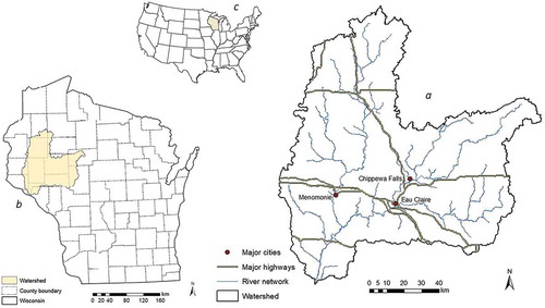
Agriculture and forest are the dominant LULC in the study area while lakes are also prominent in several areas (Wilson 2015). Primary economic activities encompass agriculture, service, and mining (West Central Wisconsin Regional Planning Commission 2010; Wilson 2015). Eau Claire, Chippewa Falls, and Menomonie are the largest cities in the watershed with a total population of 96,000 (U.S. Census Bureau 2010). Overall population within the watershed is approximately 280,000 (U.S. Census Bureau 2010).

2.2. Datasets and image processing

The data sources for this research primarily consisted of several GIS data and three set of satellite image scenes. The GIS data include decennial U.S. Census data at the block group level for 1990, 2000, and 2010, respectively (Minnesota Population Center 2011), zoning data, and the 2010 assessed land value from Wisconsin Statewide parcel data (Wisconsin State Cartographer’s Office 2017). The satellite images are from Landsat-5 Thematic Mapper (TM) satellite sensor individually acquired between August 9-September 10, 1990, 29 August –5 September 2000, and July 11–3 August 2011. TM images are available in six reflective bands at a spatial resolution of 30 m (USGS 2013a). The images are distributed by the USGS already corrected for atmospheric interference with the use of the Landsat Ecosystem Disturbance Adaptive Processing System (LEDAPS) algorithm (Schmidt et al. 2013). This study employed Landsat-5 surface reflectance data. Additionally, digital raster graphics, National Agriculture Imagery Program high resolution orthoimagery, historical aerial photograph of Wisconsin, and classified LiDAR point clouds were also used (USDA 2013; USGS 2013b; Wisconsin DNR 2013; Wisconsin State Cartographer’s Office 2017).

The current study considered a total of eight LULC classes developed by modifying the USGS Anderson Level 1 LULC classification system (Anderson et al. 1976). Classes produced include water, residential, institutional, industrial, green vegetation (GV)/shrub, forest, commercial, and agriculture. In extracting LULC information from the TM images, two individual hybrid approaches were utilized. The first involved the use of linear spectral mixture analysis (LSMA) in consonance with maximum likelihood (ML) classifier in stage 1 and an expert system in stage 2, using all reflective bands (Lu and Weng 2004; Kahya, Bayram, and Reis 2010; Wilson 2014). In a LSMA model, the spectral reflectance recorded by an orbital or sub-orbital sensor is a linear amalgam of all types of information contained in a pixel (Ridd 1995). Equation 1 demonstrates a LSMA model.

(1) $\begin{array}{c}{S}_{\mathit{i}}=\sum _{p=1}^N{t}_p{S}_{ip}+{\epsilon }_{\mathrm{i}}\end{array}$(1)

Where S_i is the reflectance signal of a pixel in spectral channel i that encapsulates single or multiple endmembers; i = 1, … j are the number of spectral channels captured by the sensor; p = 1, … m represents number of unique spectral reflectance/endmembers contained in the image; t_p is the fraction of endmember p within a pixel, S_ip is the acknowledged reflectance signature of endmember p within a pixel in spectral channel i; ε is the amount of error contained in a particular spectral channel such as i. We utilized a forward principal component rotation to transform the TM reflective bands to principal component images in a bid to collect endmembers (Wilson 2014). The following endmembers were collected: water, urban/built-up, forest, and non-forested vegetation. In converting endmembers to fractional images, we employed a constrained unmixing solution defined by Equation 2 (Wilson 2014).

(2) $\begin{array}{c}\sum _{p=1}^N{t}_p=1and0\le t_p\le 1\end{array}$(2)

The ML classifier was used to merge the fractional images thus producing stage 1 land cover data. For an in-depth description of the LSMA procedure undertaken in this study, see Wilson (2014). To arrive at detailed urban land use classes and to separate non-forested vegetation into its specific LULC classes, we used an expert system classifier (Wilson 2014). This classifier develops rules between an image and ancillary data (Kahya, Bayram, and Reis 2010). Zoning information, Google Earth images, and surface models generated from LiDAR point cloud provided ancillary data for the second stage of classification. We developed rules to integrate the ancillary data with the results obtained from stage 1 classification to produce the 8 LULC classes mentioned above.

The second hybrid classification approach combined an object-based image analysis (OBIA) and expert system classifier (Blaschke 2010; Kahya, Bayram, and Reis 2010) in two stages. An OBIA combines both the spectral and spatial characteristics of features contained in an image in extracting LULC information (Blaschke 2010). Creation of image objects was accomplished with the multiresolution segmentation algorithm while segmentation parameters for spectral and spatial characteristics of objects was guided by local variance of heterogeneity (Dragut, Tiede, and Levick 2010). Equation 3 illustrates a simplified schematic of the major parameters in the segmentation process.

(3) ${\mathrm{S}}_{\mathrm{f}}=w_c\ast h_c+\left(1-w_c\right)\ast h_s\mathrm{a}\mathrm{n}\mathrm{d}0\le w_c\le 1$(3)

Where S_f is the segmentation function; w_c is weight assigned to color; h_c represents color criterion; while h_s denotes spatial criterion. For a detailed discussion of multiresolution image segmentation, see Benz et al. (2004). The same segmentation parameter was employed for the 1990, 2000, and 2011 images as initial trials with slightly different parameters produced unexpected artifact in images with larger scale parameter. Training of image objects was facilitated by the random forest classifier (Gislason, Benediktsson, and Sveinsson 2006) informed by texture and other contextual information to derive 5 classes – urban/built-up, water, GV/shrub, agriculture, and forest. The OBIA classification result was then inputted into an expert system classifier to compartmentalize the urban/built-up land cover into its various land uses and to properly separate GV/shrub from agriculture by using the same ancillary datasets employed in the first hybrid classification approach discussed above.

In assessing the accuracy of image classification, 1000 reference points were collected for each image through stratified random sampling technique (Congalton 1991). The number of reference points allocated per LULC class vary directly with the spatial extent and structural heterogeneity of each class. To minimize bias in the accuracy assessment, the stratified random sampling further omitted all training pixels and objects that were used in hybrid classification methods 1 and 2 respectively. Reference points were obtained from historical aerial photograph of Wisconsin, the National Agriculture Imagery Program high resolution orthoimagery, and Google Earth high resolution images for the 1990, 2000, and 2011 images respectively (Wisconsin Department of Natural Resources (WDNR) 2013; USDA 2013; Google Earth 2016).

2.3. Land change driver and policy prescription development

A wide variety of land change drivers were initially identified during the search and discovery process based on consultation with regional comprehensive land use plan practitioners from the West Central Wisconsin Regional Planning Commission (WCWRPC), literature review, and expert knowledge of the dynamics of major land change drivers in the LCRW. These drivers can be categorized into socioeconomic, proximity, biophysical, probability, and policy (Table 1). Proximity related drivers were generated by a 3.2 km (2 mile) multiple ring buffer from major roads (Interstate and US highways) and the three major cities in the LCRW – Eau Claire, Chippewa Falls and Menomonie. Following spatial analysis, this buffer linear unit was used since it was found to be the most optimal for the study area. The probability driver (evidence likelihood) was calculated as an empirical probability of change between an earlier land use image (t-1) (e.g., 1990), and a later image (t) (e.g., 2000).

Table 1. Land change drivers & constraints.

Categories	Initial consideration	Final selection
Socio-economic	Housing density	o
	Population density	Y
	Median household income	Y
	Total manuf. & const. employees	o
	Total agricultural employees	o
	Total wholesale & retail employees	o
	Total service industry employees	o
	Assessed land value	Y
Proximity	Distance to major highways	Y
	Distance to major cities	Y
Biophysical	Slope	o
	Aspect	o
	Soil	o
	Elevation	o
Probability	Evidence likelihood	Y
Policy	Forest land constraint	Y
	Agricultural land constraint	Y
	Urban growth boundary constrain	Y
	Riparian vegetation constrain	Y
	Non-zoned	Y
	Zoned	Y

Note: Y included in projection, o omitted from projection,

Manuf. manufacturing, const. construction

All land change drivers were then ranked by the plan practitioners and subsequently revised with inputs from the authors according to their importance in effecting land change in the LCRW. Next, a contingency table analysis test was employed on all drivers to evaluate their predictive power. This test examined the relationship between the value of each driver within a geographic unit and that of the distribution of the current land cover map within the same geographic unit (Eastman 2016). The evaluation of the level of relationship was conducted with the Cramer’s V statistics, which is defined as follows (Rodriguez et a1. 2012):

(4) ${\mathrm{V}}_{\mathrm{c}}=\sqrt{\frac{x^2}{N\left(k-1\right)}}0\le {\mathrm{V}}_c\le 1$(4)

Where V_c denotes Cramer’s V; $x^2$ illustrate Pearson chi-square statistics; N is the sample size, and $k$ is the lesser number of categories for either the driver or current land cover map. A high Cramer’s V indicates a land change driver possess greater influence on LULC distribution. At the end of the driver evaluation process, those that were proven to have little to no influence on LULC distribution in the LCRW were omitted.

At the completion of driver evaluation for inclusion in model prediction, the next task was to identify key land use plan prescriptions from a regional comprehensive plan of the study area and to translate these qualitative drivers into a quantitative structure. The provenance of qualitative drivers is based on recommendations from the WCWRPC. The latter recommends that all contiguous forested and agricultural lands that are 40.5 hectares (100 acres) and above to be preserved from transitioning till the end of the plan’s vision period of 2030–2040. In order to translate this plan prescription into spatially explicit driver variable, forest and agricultural lands were independently extracted from the 2011 object-based hybrid classified image to create two respective binary images. The binary images were clumped and the area threshold applied to eliminate contiguous clumps that did not meet the size specification of plan prescriptions (Bunting et al. 2014). Another pivotal planning prescription adopted by the WCWRPC is the principle of smart growth (Talen and Knaap 2003). In this direction, an urban growth boundary in the Eau Claire-Chippewa Falls urban corridor and the City of Menomonee is to be developed. An urban growth boundary was created by extracting the 2011 object-based hybrid urban LULC in the aforementioned cities while masking the other LULC classes. Next, contiguous urban patches were clustered and their edges used to demarcate the 2011 urban boundary. Centroids of these patches were calculated and lateral allowable growth was guided by azimuths from the centroids, zoning, and plan prescription from the WCWRPC. The planning commission further proposed the preservation of riparian vegetation around all water bodies. We generated constraint images for these waterbodies to prevent transitions occurring within these corridors. In local jurisdictions that are devoid of zoning, land transition was described as excessive by the plan practitioners. This non-zoned policy driver in some jurisdictions is normally leveraged by local politicians in encouraging flexibility in land change within the affected areas. In order to translate this qualitative policy driver into a spatially-explicit structure, we tracked the LULC transitions per class within the affected areas over a 21-year period (1990–2000, 2000–2011) to obtain an estimate of the spatial extent of change resulting from the lack of zoning.

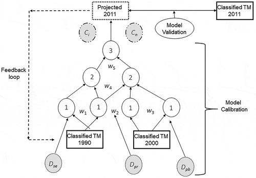
After configuring land change drivers into a quantitative form, the next procedure was to arrive at an optimal spatially-explicit format. This exercise, often referred to as model calibration, was facilitated by a dynamic simulation model that integrates multi-layer perceptron (MLP) neural network and Markov Chain – MC (Eastman 2016). The MLP-MC model was adopted to develop functional relationships between selected land change drivers and the spatial extent and trajectory of change patches. As a feed-forward artificial neural network with multiple layers that span input (land change drivers, policy prescriptions), hidden (nodes and neurons), and output (transition probability), it learns through the complex connections between input and output nodes in understanding the dynamics of land change drivers (Qiu and Jensen 2004). At the end of the learning process, the MLP generates transition probability maps from one LULC class to another (Eastman 2016). The transition probability maps are then fed into a Markov Chain (MC) to make projections of LULC. In a MC, the probability p(y_t) that a phenomenon exist in state a_j if it was in state a_i at a previous time is denoted by the following equation:

(5) $\mathrm{p}⟨y_t=a_j|y_{t-1}=a_i⟩$(5)

A landscape such as the LCRW is characterized by various states or LULC configurations which is dynamic over time (Table 2). Equation 6 depicts a Markov Chain matrix that encapsulates multiple transitions such as that illustrated in Table 2.

(6) $\underset{\_}{P}=\left[p_{ij}\right]=\left[\begin{array}{c}{p}_{11},p_{12,}...p_{1n}\\ p_{21},p_{22,}...p_{2n}\\ p_{n1},p_{n2,}...p_{nn}\end{array}\right]$(6)

Table 2. LULC trajectory used in creating probability/transition potential Surfaces.

		To
		water	Commercial	Forest	GV/S	Residential	Institutional	Agriculture	Industrial
From	Water	–	Y	N	Y	Y	Y	Y	Y
	Commercial	N	–	N	N	Y	Y	N	Y
	Forest	Y	Y	–	Y	Y	Y	Y	Y
	GV/S	Y	Y	N	–	Y	Y	Y	Y
	Residential	N	N	N	N	–	N	N	N
	Institutional	N	N	N	N	N	–	N	N
	Agriculture	N	Y	Y	Y	Y	Y	–	Y
	Industrial	Y	Y	N	Y	Y	Y	Y	–

Note: Y included, N not included, – not applicable, GV/S green vegetation/shrub.

Where P = $\left[p_{ij}\right]$ is the probability of transitioning from one state _i to a different state _j or to multiple states (_{i1, i2,….ij}). We individually trained the MLP-MC with the 1990 and 2000 hybrid pixel-based and hybrid object-based LULC maps respectively to simulate two 2011 images. Land change drivers employed during this stage include the final selected socioeconomic, proximity, probability, non-zoned, and zoned policy (Table 1). The policy related constraints were not employed here because they were not part of the older regional comprehensive plan that governed the period before 2010. Among the 56 possible transitions from the eight LULC types between 1990 and 2000, only 34 of them were observed to be significant in both hybrid pixel and hybrid object input LULC cases and hence used to produce related transition probability maps by the MLP (Table 2).

During model calibration, the population density and median household income socioeconomic drivers were initially inputted at their 1990 and 2000 values but subsequently, a calculated difference image between the two years worked better. In encoding the behavior of the non-zoned policy driver into the MLP-MC model, maximum incentive for land transition was embedded into these non-zoned lands. On the other hand, lower incentives was inserted in zoned lands to depict the varying levels of flexibility of land transition in non-zoned lands vis-à-vis areas characterized by zoned policy. In order to prevent future transition in areas that are zoned as protected, no incentive was allocated to these areas as they are meant to remain static in the future.

2.4. Model validation and development of projected images

Validated was accomplished by comparing the 2011 classified images with the simulated LULC images of the same year (Figure 2). We employed the Relative Operating Characteristics (ROC) tool to assess the efficacy of the models (Mas et al. 2013). In the standard approach of ROC implementation, the probability/transition potential surface map used in generating the projected land use data is divided into suitability groups according to the levels of probability and area threshold (for e.g. 0–10%, 10–20%, ….. 90–100%) which is then compared with the real world classified map of that same time (Pontius and Schneider 2001). The resultant ROC information/graph is then used to compute the Area Under the Curve (AUC) statistics to determine the performance of land change models (Mas et al. 2013). The AUC statistics is calculated as follows:

(7) $\mathrm{A}\mathrm{U}\mathrm{C}=\sum _{t=1}^n\left[x_{t+1}-x_t\right]\left[yt+y_{t+1}-y_t/2\right]$(7)

Figure 2. Projected land use data model construction.

Note: D_se socioeconomic drivers, D_pr proximity drivers, D_pb probability driver, 1–3 perceptron, w weights, C_i first constraint (e.g. forest), C_n last constraint (e.g. urban growth boundary).

Where x_t represents the rate of false positives for scenario t, y_t denotes the rate of true positives for scenario t, and n is the number of suitability groups. The AUC produces a result between 0 and 1, where 1 represents a perfect model and less than 0.5 suggests that the model has less predictive efficacy than a random probability map (Mas et al. 2013). In this study, a pair of AUC was calculated for the two projected 2011 LULC images with all classes as a whole and individual classes as well.

In developing the projected images for 2030 and 2050, the calibrated and validated MLP-MC model with input from the 2000 and 2011 object-based hybrid classified LULC maps was employed. We chose the object-based hybrid classified input images for future projection because it produced better validation results compared to the pixel-based hybrid classified images. Transition constraints were applied to the forest and agricultural policy drivers to prevent conversion of those cells in the development of future LULC data. Transition constraint was also established within riparian vegetation corridors. Urban growth boundary constraint was imposed on residential, commercial and institutional lands related to the build-up area.

3. Results

3.1 Historical and contemporary images: production accuracy and landscape trajectory

Figure 3 illustrates the overall accuracy (OA) for the pixel-based hybrid and object-based hybrid approaches employed in this study. The object-based hybrid approach performed slightly better than the pixel-based method for each of the three years with an average of 1.8% increase in OA (p < 0.05). Tables 3 and 4 lists the producers and users accuracy for each date of classified image for the pixel-based hybrid and the object-based hybrid methods respectively. A more detailed examination of the performance of the classification approaches at the individual class level reveals that there are instances when the pixel-based hybrid approach performed better than the object-based method. For e.g., Tables 3 and 4 demonstrate that the pixel-based hybrid approach produced better users accuracy for commercial and institutional classes for all years. Additionally, the pixel-based hybrid approach produced slightly better users accuracy for GV/shrub and agriculture classes for some years. When the producers accuracy was closely examined, the object-based hybrid approach outperformed the pixel-based method for all classes with the exception of forest and to some extent industrial class.

Figure 3. Comparison of overall accuracy for historical and contemporary images.

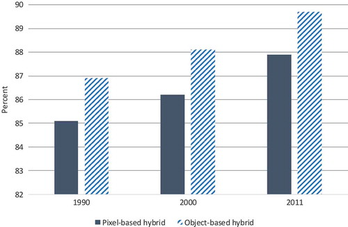
Table 3. Producers and users accuracy for pixel-based hybrid classified images.

		Water	Comm	Forest	GV/S	Residential	Inst	Agric	Indst
1990	PA(%)	98	77	92	73	75	88	79	81
	UA(%)	95	94	83	95	86	97	95	91
2000	PA(%)	94	76	89	63	78	67	75	89
	UA(%)	93	100	82	91	85	96	96	79
2011	PA(%)	98	89	98	71	89	67	72	92
	UA(%)	99	97	80	84	94	100	86	80

Note: comm commercial, GV/S green vegetation/shrub, Inst institutional, Agric agriculture, Indst industrial, PA producer’s accuracy, UA user’s accuracy.

Table 4. Producers and users accuracy for object-based hybrid classified images.

		Water	comm	Forest	GV/S	Residential	Inst	Agric	Indst
1990	PA(%)	98	81	91	77	83	86	87	85
	UA(%)	96	91	87	86	86	92	93	91
2000	PA(%)	96	86	92	73	84	84	84	79
	UA(%)	94	84	85	82	86	92	90	89
2011	PA(%)	98	90	94	81	92	82	85	84
	UA(%)	96	84	86	87	95	95	91	87

Note: comm commercial, GV/S green vegetation/shrub, Inst institutional, Agric agriculture, Indst industrial, PA producer’s accuracy, UA user’s accuracy.

Figure 4 illustrates the three LULC maps derived from the object-based hybrid classification for 1990, 2000, and 2011, respectively. Change analysis of the maps indicates that residential, commercial, industrial, and insitutional lands experienced significant increase over the assessment period while net losses were incurred in forest, GV/shrub, and agriculture (Figure 5). Most of the lands that transitioned to residential and other urban uses between 1990 and 2011 are from forest, agriculture, and to some extent GV/shrub (Table 5).

Table 5. Land use/land cover net gain transition matrix (hectares).

		To 2011
		water	Commercial	Forest	GV/S	Residential	Institutional	Agriculture	Industrial
From 1990	Water	–	17	0	0	231	10	12	3
	Commercial	0	–	0	0	0	0	0	0
	Forest	502	283	–	98	5882	78	9026	496
	GV/S	100	18	53	–	286	13	425	17
	Residential	0	0	0	0	–	0	0	0
	Institutional	0	0	0	0	7	–	0	0
	Agriculture	0	426	30	18	6789	301	–	475
	Industrial	10	0	0	7	21	11	15	–

Note: – not applicable, GV/S green vegetation/shrub.

Figure 4. Historical and contemporary object-based hybrid classified images for 1990 (a), 2000 (b), and 2011 (c).

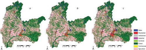
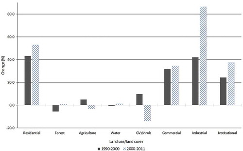
Figure 5. Percentage change in LULC, 1990–2011.

Note: GV green vegetation.

3.2 Future landscape: model performance and potential landscape trajectory

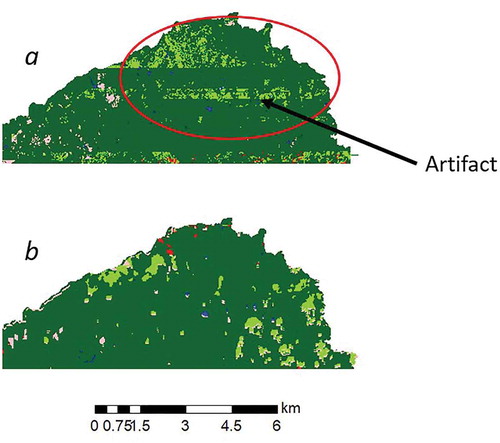
Model calibration demonstrated that the most optimal configuration for the MLP-MC model was a population density change image between 1990 and 2000. This implies that the trend format, rather than individual year’s representation of population driver can best support the MLP-MC model to learn trajectories between different years. This breakthrough in spatially configuring population driver provided valuable clues for incorporating other socioeconomic drivers into the land change model. Another pivotal observation was that iteratively rescaling the absolute assessed land value driver into ranges assisted the MLP-MC model during the learning process. Additionally, the encoding of various levels of incentives and constraint on policy related drivers demonstrated a closer replication of real world land transitions by the MLP-MC model. Results further demonstrated that the 2011 projected image from the pixel-based hybrid classification maps generated conspicuous artifacts despite comparable classification accuracy to the object-based hybrid method. When the object-based hybrid input images were employed in simulation, a more reliable predicted image with no artifact was produced. Figure 6a shows a snippet of the northeastern LCRW with GV/shrub artifact from the pixel-based hybrid method while the object-based hybrid approach (Figure 6b) is devoid of this problem. Since the same model driver configuration was used to generate the 2011 projected images with the only exception of pixel-based hybrid input baseline images versus object-based hybrid input baseline images, we can attribute the artifacts mentioned above to the mostly heterogeneously-oriented structure of the pixel-based hybrid input images. We speculate that during the projection of the 2011 image from the pixel-based hybrid input, the model might have struggled with translating the “salt and pepper” heterogenous structured transition potential surfaces derived from pixel-based hybrid input images to a structurally homogeneous projected surface. Another important observation is that this artifact was mostly detected in areas where the LULC is fragmented and was solely extracted based on pixel information alone (GV/shrub and agriculture). The ancillary data used to extract the urban land uses in stage 2 of pixel-based hybrid classification encoded a more homogenous structure into residential and other urban land uses thus forestalling the creation of artifacts. Moreover, forest cover displayed less amount of fragmentation compared to GV/shrub and agriculture and thus preserved a relatively homogenous structure with minimal artifacts from pixel-based hybrid method.

Figure 6. Snippet of 2011 pixel-based hybrid projected image (a) compared to object-based hybrid (b).

The calibrated model with input from object-based hybrid LULC maps performed better than the pixel-based hybrid with an average improvement of 0.15 in AUC value (Figure 7).

Figure 7. Average ROC performance of model for all projected 2011 LULC classes.

Note: AUC_O is object-based hybrid, AUC_P is pixel-based hybrid.

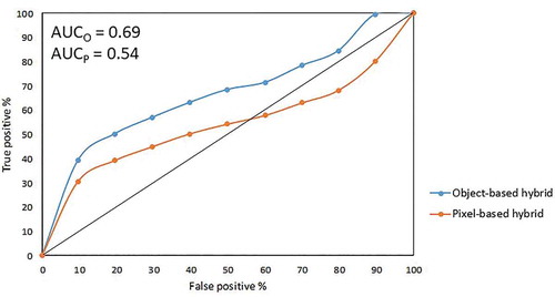
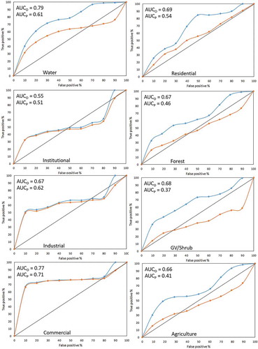
The better overall performance of the object-based hybrid input LULC model can be attributed to the lack of projection artifact in GV/shrub, agriculture, and forested areas. It is pivotal to evaluate the spatial performance of model efficiency within the lens of LULC composition and configuration rather than just limiting validation to overall model performance especially when such datasets have potential to be used for policy formulation. Figure 8 presents the ROC validation curves and AUC values for the eight projected LULC classes from the two sets of input LULC maps. The graphs shows that the model with input from object-based hybrid classified maps performed better compared to the pixel-based hybrid for all classes though with varying levels of differences per class. For most of those classes delineated during stage 2 of classification (Institutional, industrial, and commercial), difference in AUC scores between the object-based hybrid and pixel-based hybrid was within 6% (Figure 8). In fact, at higher suitability thresholds for some of these classes, model performance was identical. On the contrary, LULC classes that were wholly or partially delineated during stage 1 of classification (agriculture, GV/shrub, forest) demonstrated the greatest difference in AUC scores (15% ≤ 31%). We ascribe the larger difference in model performance for these classes to the artifact generated by pixel-based hybrid model causing errors in projection. With the exception of residential, such projection artifacts was non-existent in classes mostly delineated in stage 2 of image classification from the pixel-based hybrid LULC input data.

Figure 8. ROC performance of models per projected 2011 LULC class.

Note: AUC_O is object-based hybrid

, AUC_P is pixel-based hybrid.

Additionally, we probed into areas where the models missed transitions for the LULC classes. Misses and falls alarms for the object-based hybrid input model were mostly found in proximate locations (< 3.2 km) to the major cities in the LCRW while those for the pixel-based hybrid were located within and outside the aforementioned area. The poor performance of both models close to major urban centers can be explained by the complexity of urban landscape within and around cities.

Figure 9 displays the 2011 object-based hybrid classified map together with the projected maps for 2030 and 2050. The projected maps suggest that residential land in the LCRW will continue to grow up till 2050 though at a slower rate (< 20%) compared to the historical (1990–2000) and contemporary (2000 – 2011) epoch (Figure 6).This slower rate of residential land expansion can be attributed to the implementation of smart growth where an urban growth boundary is established and the enforcement of plan prescription of a cap in areal extent threshold for forest and agricultural land transition.

Figure 9. Contemporary and projected images for 2011 (a), 2030 (b), and 2050 (c).

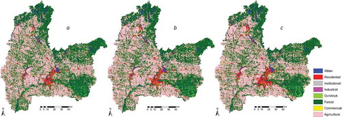
Most of the growth in residential land (Figure 9b and 9c) is slated to occur in the southeastern portion of the Eau Claire-Chippewa Falls urban corridor while the southwestern portion is poised to experience a slower expansion in residential lands. This differential can be attributed to higher land value and potential for growth in that portion of the Eau Claire-Chippewa Falls urban corridor compared to other zones. Slight increase in residential land is also projected to occur in the northwestern portion of the Eau Claire-Chippewa Falls urban corridor (Figure 9b and 9c). Growth in the areal extent of residential land in the LCRW is anticipated to occur partly as a response to population growth from its associated driver encoded during model construction. Figure 10 demonstrates that commercial and institutional lands are expected to grow at an average of 17 and 12% respectively over the forecast period.

Figure 10. Potential percentage change in LULC, 2011–2050.

Note: GV green vegetation.

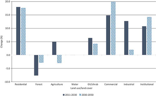
The model suggests that industrial land will continue to increase throughout the forecast period though at a slower rate (17%) compared to the baseline period (86.4%) of 2000 and 2011. The model projected slight increase in industrial lands in proximate location to the major cities over the forecast period. This can be ascribed to a response to higher income and land value closer to cities compared to areas farther out. Agricultural land is projected to experience relatively notable increase by 2030 but a slight drop by 2050 (Figure 10). To make room for the increase by 2030, some forested land below the size constraint were transitioned to agricultural land. The slight decline of agricultural land by 2050 can be traced to model uncertainty as one would expect the same trend of increase to continue beyond 2030. Additional forest decline is projected to be caused by increase in GV/shrubs.

4. Discussion

The major drivers of land change in the LCRW between 1990 and 2011 are population growth, technological, and income (Wilson 2015). This study demonstrated that residential, commercial, and institional land uses between 1990 and 2011 increased in response to population growth (> 10%) and its antecedant service needs over the study period (U.S. Census Bureau 2010). Growth in industrial lands, especially during the 2000–2011 period, can be attributed to the accentuation of industral sand mining in response to the high demand for industrial sand by the oil and gas industry to support hydraulic fracturing. Across the LCRW, there are approximately 46 industrial sand mines which constitues 41% of the state’s total (Wisconsin DNR 2015). A number of studies have reported that anthropogenic drivers are the main impetus of land change in areas of human habitation (Lambin et al. 2001; Wilson and Wilson 2016). Projected images of 2030 and 2050 demonstrated that a similar trend of land change is expected to occur though at a slower rate. The latter can be attributed to the policy related constraints encoded into the MLP-MC model. Our model result is in consonance with similar studies that have concluded that an urban area which has experienced population and economic growth is most likely to continue in this direction in the future (Alcamo et al. 2011; Wilson and Weng 2011). Such urban expansion has been shown to manifest in a controlled and non-sprawl manner when the principle of smart growth is applied (Song and Knaap 2004; Wassmer 2006).

This study has demonstrated that both pixel-based hybrid and object-based hybrid classified LULC maps can be used as baseline images in an MLP-MC land change model to project future LULC data. A component of this finding tend to resonate with other studies that have used baseline images created with either of these methods (Onate-Valdivieso and Sendra 2010; Wilson and Weng 2011; Tayyebi and Pijanowski 2014). Results of this current study goes further to evaluate the efficacy of the two methods for LULC baseline maps and has demonstrated that LULC baseline maps created with an object-based hybrid method resulted in more accurate projected image compared to that generated with the pixel-based method. The improved overall and individual class AUC values from the validation analysis of the MLP-MC model informed by object-based hybrid classified LULC maps can be attributed to its more spatially homogenous units (patches) compared to a heterogeneously-oriented analysis (pixel) from the pixel-based hybrid classified LULC maps. Scholars have widely reported the “salt and pepper” effect synonymous with per-pixel classifiers (Ouyang et al. 2011; Whiteside, Boggs, and Maier 2011). However, this reported case of apparent stripe artifact generated by some LULC classes from the pixel-based-hybrid input images in consonance with the “salt and pepper effect” appears to be a new and additional anomalous phenomenon in land change prediction analysis, especially with the MLP-MC method used in this study. While more research efforts are called on to look into this issue, we recommend that an OBIA should precede post-classification sorting algorithms such as Expert System for moderate spatial resolution images rather than a per-pixel classifier before inclusion in a land change projection model. Alternatively, a convolution filter can be implemented on pixel-based hybrid baseline images for land change projections to eliminate the ‘salt and pepper effect (Onate-Valdivieso and Sendra 2010) and also potentially preclude the formation of artifacts.

The rigorous validation approach undertaken in this study to probe into the locations of wrong projected pixels and patches within the study area is pivotal for two reasons. First, to obtain a sense of the spatial and contextual characteristics of those areas and second, to potentially develop spatial constraints for some of those areas that fall within protected or inflexible zoned areas. Most of the missed areas were found in public lands that are adjacent to areas with relatively high land values, and witnessed increase in population and income between 1990 and 2000. The MLP-MC assumed that these public lands might be transitioning since some of them were deliberately excluded from model construction in a bid to reduce model complexity. To improve model performance in these locations when possible, publics lands should be fully encoded into the model in the form of spatial constraints to prevent incorrect transitions from taking place in those locations (Verburg, Tabeau, and Hatna 2013; Schaldach et al. 2011; Pindozzi et al. 2017). Additionally, model uncertainty was high close to the major urban centers in the LCRW. In an effort to minimize errors in model prediction for these areas, we recommend that appropriate constraints and diverse ranges of incentives be implemented within and around complex urban corridors.

Another pivotal finding from this study is the importance of configuring land change drivers during model calibration. Our result illustrates that the way in which an individual land change driver is spatially configured could play an important role in the learning process and hence the efficacy of the land change model. This issue was seldom addressed in previous studies on which the focus was mainly on the entire driver-landscape system instead of an individual driver. For instance, system dynamics (Schmitt Olabisi et al. 2010), fuzzy cognitive maps (Jetter and Kok 2014), agent-based modeling (Parker et al. 2003), and related models are geared towards understanding the behavior of land change drivers in a system in order to obtain coefficients for parameterizing model variables. Most of these models have been successful in simulating future LULC scenarios (Tayyebi and Pijanowski 2014; Mas et al. 2014). Notwithstanding, the apparent dearth of information on how to correctly spatially configure individual land change drivers for specific model architecture such as the MLP-MC used in this study can result in an increase in model uncertainty if such input datasets are not structured correctly. It might be beneficial for a research to be conducted on the spatial configuration of diverse land change drivers for specific simulation models.

5. Conclusion

This study has demonstrated that even though both pixel-based hybrid and object-based hybrid classification algorithms can be used to project future LULC data, validation results illustrates that the object-based hybrid classified input images resulted in the projection of more accurate results. This outcome connotes that the choice of image classification algorithm is critical not only in yielding useful LULC information, but also in successfully informing land change modeling in generating more accurate projected images as well – a topic seldom addressed in the past. Results further shows that the calculation of differences to generate trends in socioeconomic drivers is more effective than using independent timescale when training a MLP-MC land change model. The projected images suggests that the areal extent of urban LULC, including GV/shrub, will continue to increase till 2050 though at a slower rate compared to the baseline period. It might be prudent to test the two hybrid classification approaches adopted in this study on other land change models to verify whether the artifact reported from a pixel-based hybrid method is reproducible. Overall, the measures used in this study are observed to be efficient in filtering out land change drivers that have little to no influence on model efficacy. In general, the modeling framework developed in this study can be easily adopted to other watersheds irrespective of spatial scale, complexity in LULC composition, configurations, and driver dynamics. This allows for a better understanding of the relationships between LULC and all sorts of drivers such as policy, technological, and socioeconomic at diverse spatial and temporal scales. It therefore lays the foundation for enhancing the understanding of the impacts of short-to-medium term land use decision-making processes on water resource sustainability.

Acknowledgments

This research is sponsored by the Office of Research and Sponsored Programs and the Department of Geography and Anthropology, University of Wisconsin-Eau Claire. The authors wishes to thank senior planners of the West Central Wisconsin Regional Planning Commission for their invaluable inputs throughout this project. Finally, the authors would like to express gratitude to three anonymous individuals for providing pivotal suggestions that helped improve the manuscript and also all those who gave positive feedback on the research during several conference presentations.

Disclosure statement

No potential conflict of interest was reported by the authors.

Additional information

Funding

This work was supported by the Office of Research and Sponsored Programs and the Department of Geography and Anthropology, University of Wisconsin-Eau Claire.

References

- Agarwal, C., G. M. Green, J. M. Grove, T. P. Evans, and C. M. Schweik. 2002. “A Review and Assessment of Land-Use Change Models: Dynamics of Space, Time, and Human Choice.” General Technical Report NE-297. USDA Forest Service, Northeastern Research Station.
- Alcamo, J., R. Schaldach, J. Koch, C. Kolking, D. Lapola, and J. Priess. 2011. “Evaluation of an Integrated Land Use Change Model Including a Scenario Analysis of Land Use Change for Continental Africa.” Environmental Modelling & Software 26: 1017–1027. doi:10.1016/j.envsoft.2011.03.002.
- Anderson, J. R., E. E. Hardy, J. T. Roach, and R. E. Witmer. 1976. “A Land Use and Land Cover Classification System for Use with Remote Sensor Data.” U.S. Geological Survey Professional Paper 964, 28 pp. Washington, D.C., U.S. Government Printing Office.
- Benz, U. C., P. Hofmann, G. Willhauck, I. Lingenfelder, and M. Heynen. 2004. “Multi-Resolution, Object-Oriented Fuzzy Analysis of Remote Sensing Data for GIS Ready Information.” ISPRS Journal of Photogrammetry & Remote Sensing 58: 239–258. doi:10.1016/j.isprsjprs.2003.10.002.
- Blaschke, T. 2010. “Object Based Image Analysis for Remote Sensing.” ISPRS Journal of Photogrammetry & Remote Sensing 65: 2–16. doi:10.1016/j.isprsjprs.2009.06.004.
- Boucher, A., K. C. Seto, and A. G. Journel. 2006. “A Novel Method for Mapping Land Cover Changes: Incorporating Time and Space with Geostatistics.” IEEE Transactions on Geoscience and Remote Sensing 44 (11): 3427–3435. doi:10.1109/TGRS.2006.879113.
- Bradley, A. V., I. Rosa, R. G. Pontius, S. E. Ahmed, M. B. Araujo, D. G. Brown, A. Brandao, et al. 2016. “SimiVal, a Multi-Criteria Map Composition Tool for Land-Change Model Projections.” Environmental Modelling & Software 82: 229–240. doi:10.1016/j.envsoft.2016.04.016.
- Bunting, P., D. Clewley, R. M. Lucas, and S. Gillingham. 2014. “The Remote Sensing and GIS Software Library (Rsgislib).” Computers & Geosciences 62: 216–226. doi:10.1016/j.cageo.2013.08.007.
- Congalton., R. G. 1991. “A Review of Assessing the Accuracy of Classification of Remotely Sensed Data.” Remote Sensing of the Environment 37: 35–46. doi:10.1016/0034-4257(91)90048-B.
- Dragut, L., D. Tiede, and S. R. Levick. 2010. “ESP: A Tool to Estimate Scale Parameter for Multiresolution Image Segmentation of Remotely Sensed Data.” International Journal of Geographic Information Science 24 (6): 859–871. doi:10.1080/13658810903174803.
- Eastman, J. R. 2016. TerrSet Geospatial Monitoring and Modeling System Manual. Worcester: Clark Labs, Clark University.
- El-Khoury, A., O. Seidou, D. R. Lapen, M. Sunohara, Q. Zhenyang, M. Mohammadian, and B. Daneshfar. 2014. “Prediction of Land-Use Conversions for Use in Watershed-Scale Hydrological Modeling: A Canadian Case Study.” The Canadian Geographer 58 (4): 499–516. doi:10.1111/cag.12105.
- Gislason, P. O., J. A. Benediktsson, and J. R. Sveinsson. 2006. “Random Forests for Land Cover Classification.” Pattern Recognition Letters 27 (4): 294–300. doi:10.1016/j.patrec.2005.08.011.
- Google Earth. 2016. Google Earth Pro (Version 7.1.2.2041) [Software]. Mountain View, CA: Google Earth. Accessed 29 June 2016.
- Guan, D., H. Li, T. Inohae, W. Su, T. Nagaie, and K. Hokao. 2011. “Modeling Urban Land Use Change by the Integration of Cellular Automaton and Markov Model.” Ecological Modelling 222: 3761–3772. doi:10.1016/j.ecolmodel.2011.09.009.
- Jetter, A. J., and K. Kok. 2014. “Fuzzy Cognitive Maps for Futures Studies – A Methodological Assessment of Concepts and Methods.” Futures 61: 45–57. doi:10.1016/j.futures.2014.05.002.
- Kahya, O., B. Bayram, and S. Reis. 2010. “Land Cover Classification with an Expert System Approach Using Landsat ETM Imagery: A Case Study of Trabzon.” Environmental Monitoring and Assessment 160: 431–438. doi:10.1007/s10661-008-0707-6.
- Lambin, E. F., M. D. Rounsevell, and H. J. Geist. 2000. “Are Agricultural Land-Use Models Able to Predict Changes in Land-Use Intensity?” Agriculture, Ecosystems and Environment 82: 321–331. doi:10.1016/S0167-8809(00)00235-8.
- Lambin, E. F., B. L. Turner, H. J. Geist, S. B. Agbola, A. Angelsen, J. W. Bruce, O. T. Coomes. et al. 2001. “The Causes of Land-Use and Land-Cover Change: Moving beyond the Myths.” Global Environmental Change 11: 261–269. doi: 10.1016/S0959-3780(01)00007-3.
- Li, G., D. Lu, E. Moran, L. Dutra, and M. Batistella. 2012. “A Comparative Analysis of ALOS PALSAR L-Band and RADARSAT-2 C-Band Data for Land-Cover Classification in A Tropical Moist Region.” ISPRS Journal of Photogrammetry and Remote Sensing 70: 26–38. doi:10.1016/j.isprsjprs.2012.03.010.
- Ligmann-Zielinska, A., and P. Jankowski. 2010. “Exploring Normative Scenarios of Land Use Development Decisions with an Agent-Based Simulation Laboratory.” Computers, Environment and Urban Systems 34: 409–423. doi:10.1016/j.compenvurbsys.2010.05.005.
- Lopez, E., G. Bocco, M. Mendoza, and E. Duhau. 2001. “Predicting Land Cover and Land Use Change in the Urban Fringe: A Case in Morelia City, Mexico.” Landscape and Urban Planning 55 (4): 271–285. doi:10.1016/S0169-2046(01)00160-8.
- Lu, D., P. Mausel, M. Batistella, and E. Moran. 2004. “Comparison of Land-Cover Classification Methods in the Brazilian Amazon Basin.” Photogrammetric Engineering & Remote Sensing 70 (6): 723–731. doi:10.14358/PERS.70.6.723.
- Lu, D., and Q. Weng. 2004. “Spectral Mixture Analysis of the Urban Landscape in Indianapolis with Landsat ETM+ Imagery.” Photogrammetric Engineering and Remote Sensing 70 (9): 1053–1062. doi:10.14358/PERS.70.9.1053.
- Mallampalli, V. R., G. Mavrommati, J. Thompson, M. Duveneck, S. Meyer, A. Ligmann-Zielinska, C. G. Druschke, et al. 2016. “Methods for Translating Narrative Scenarios into Quantitative Assessments of Land Use Change.” Environmental Modelling & Software 82: 7–20. doi:10.1016/j.envsoft.2016.04.011.
- Martin, L. 1965. The Physical Geography of Wisconsin. Madison, WI: University of Wisconsin Press.
- Mas, J., B. S. Filho, R. G. Pontius, M. F. Gutierrez, and H. Rodrigues. 2013. “A Suite of Tools for ROC Analysis of Spatial Models.” ISPRS International Journal of Geo-Information 2: 869–887. doi:10.3390/ijgi2030869.
- Mas, J., M. Kolb, M. Paegelow, M. T. Olmedo, and T. Houet. 2014. “Inductive Pattern-Based Land Use/Land Cover Change Models: A Comparison of Four Software Packages.” Environmental Modelling & Software 51: 94–111. doi:10.1016/j.envsoft.2013.09.010.
- Minnesota Population Center. 2011. National Historical Geographic Information System: Version 2.0. Minneapolis, MN: University of Minnesota. Accessed 24 June 2013. http://www.nhgis.org
- Mountrakis, G., J. Im, and C. Ogole. 2011. “Support Vector Machines in Remote Sensing: A Review.” ISPRS Journal of Photogrammetry and Remote Sensing 66: 247–259. doi:10.1016/j.isprsjprs.2010.11.001.
- Myint, S. W., P. Gober, A. Brazel, S. Grossman-Clarke, and Q. Weng. 2011. “Per-Pixel Vs. Object-Based Classification of Urban Land Cover Extraction Using High Spatial Resolution Imagery.” Remote Sensing of Environment 115 (5): 1145–1161. doi:10.1016/j.rse.2010.12.017.
- National Climate Data Center. 2016. “Land-Based Station Data.” Accessed 12 June 2016 http://www.ncdc.noaa.gov/
- National Research Council. 2013. Advancing Land Change Modeling: Opportunities and Research Requirements (committee members: Brown, D., Band, L.E., Green, K.O., Irwin, E.G., Jain, A., Lambin, E.F., Pontius, R.G., Seto, K.C., Turner, II B.L., Verburg, P.H.). Washington, DC: National Academies Press.
- O’Sullivan, D., and P. M. Torrens. 2000. “Cellular Models of Urban Systems.” In: Theoretical and Practical Issues on Cellular Automata, edited by S. Bandini and T. Worsch, 108–116. London: Springer. available at http://www.casa.ucl.ac.uk/cellularmodels.pdf
- Onate-Valdivieso, F., and J. B. Sendra. 2010. “Application of GIS and Remote Sensing Techniques in Generation of Land Use Scenarios for Hydrological Modeling.” Journal of Hydrology 395: 256–263. doi:10.1016/j.jhydrol.2010.10.033.
- Ouyang, Z., M. Zhang, X. Xie, Q. Shen, H. Guo, and B. Zhao. 2011. “A Comparison of Pixel-Based and Object-Oriented Approaches to VHR Imagery for Mapping Saltmarsh Plants.” Ecological Informatics 6 (2): 136–146. doi:10.1016/j.ecoinf.2011.01.002.
- Parker, D. C., S. M. Manson, M. A. Janssen, M. J. Hoffmann, and P. Deadman. 2003. “Multi-Agent Systems for the Simulation of Land-Use and Land-Cover Change: A Review.” Annals of the Association of American Geographers 93 (2): 314–337. doi:10.1111/1467-8306.9302004.
- Penha, A. M., A. Chambel, M. Murteira, and M. Morais. 2016. “Influence of Different Land Uses on Ground Water in Southern Portugal.” Environmental Earth Sciences 75: 622. doi:10.1007/s12665-015-5038-7.
- Pindozzi, S., E. Cervelli, P. F. Recchi, A. Capolupo, and L. Boccia. 2017. “Predicting Land Use Change on a Broad Area: Dyna-CLUE Model Application to the Litorale Domizio-Agro Aversano (Campania, South Italy).” Journal of Agricultural Engineering 48 (s1): 657. doi:10.4081/jae.2017.657.
- Plantinga, A., and D. Lewis. 2013. “Landscape Simulations with Econometric-Based Land-Use Models.” In: The Oxford Handbook of Land Economics, edited by J. M. Duke and J. Wu. New York: Oxford University Press, 800 pp.
- Pontius, R. G., W. Boersma, J. Castella, K. Clarke, T. de Nijs, C. Dietzel, Z. Duan, et al. 2008. “Comparing the Input, Output, and Validation Maps for Several Models of Land Change.” The Annals of Regional Science 42 (1): 11–37. doi:10.1007/s00168-007-0138-2.
- Pontius, R. G., and L. C. Schneider. 2001. “Land-Cover Change Model Validation by an ROC Method for the Ipswich Watershed, Massachusetts, USA.” Agriculture, Ecosystems and Environment 85: 239–248. doi:10.1016/S0167-8809(01)00187-6.
- Qiu, F., and J. R. Jensen. 2004. “Opening the Black Box of Neural Networks for Remote Sensing Image Classification.” International Journal of Remote Sensing 25 (9): 1749–1768. doi:10.1080/01431160310001618798.
- Ridd, M. K. 1995. “Exploring a V-I-S (Vegetation-Impervious Surface-Soil) Model for Urban Ecosystem Analysis through Remote Sensing: Comparative Anatomy for Cities.” International Journal of Remote Sensing 16 (12): 2165–2185. doi:10.1080/01431169508954549.
- Rodrıguez, N., D. Armenteras, and J. Retana. 2012. “Land Use and Land Cover Change in the Colombian Andes: Dynamics and Future Scenarios.” Journal of Land Use Science 8 (2): 154–174. doi:10.1080/1747423X.2011.650228.
- Rounsevell, M. D., I. Reginster, M. B. Araujo, T. R. Carter, N. Dendoncker, F. Ewert, J. I. House, et al. 2006. “A Coherent Set of Future Land Use Change Scenarios for Europe.” Agriculture, Ecosystems & Environment 114: 57–68. doi:10.1016/j.agee.2005.11.027.
- Scanlon, B. R., R. C. Reedy, D. A. Stonestrom, D. E. Prudic, and K. F. Dennehy. 2005. “Impact of Land Use and Land Cover Change on Ground Water Recharge and Quality in the Southwestern US.” Global Change Biology 11: 1577–1593. doi:10.1111/j.1365-2486.2005.01026.x.
- Schaldach, R., J. Alcamo, J. Koch, C. Kolking, D. M. Lapola, J. Schungel, and J. A. Priess. 2011. “An Integrated Approach to Modelling Land-Use Change on Continental and Global Scales.” Environmental Modelling & Software 26: 1041–1051. doi:10.1016/j.envsoft.2011.02.013.
- Schmidt, G. L., C. B. Jenkerson, J. Masek, E. Vermote, and F. Gao. 2013. “Landsat Ecosystem Disturbance Adaptive Processing System (LEDAPS) Algorithm Description.” U.S. Geological Survey Open-File Report 2013–1057, 17.
- Schmitt Olabisi, L. K., A. R. Kapuscinski, K. A. Johnson, P. B. Reich, B. Stenquist, and K. J. Draeger. 2010. “Using Scenario Visioning and Participatory System Dynamics Modeling to Investigate the Future: Lessons from Minnesota 2050.” Sustainability 2: 2686–2706. doi:10.3390/su2082686.
- Shu, Y., H. Tang, J. Li, T. Mao, S. He, A. Gong, Y. Chen, and H. Du. 2015. “Object-Based Classification of VHR Panchromatic Satellite Images by Combining the HDP and IBP on Multiple Scenes.” IEEE Transactions on Geoscience and Remote Sensing 53 (11): 6148–6162. doi:10.1109/TGRS.2015.2432856.
- Sohl, T. L., K. L. Sayler, M. A. Bouchard, R. R. Reker, A. M. Friesz, S. L. Bennett, B. M. Sleeter, et al. 2014. “Spatially Explicit Modeling of 1992-2100 Land Cover and Forest Stand Age for the Conterminous United States.” Ecological Applications 24 (5): 1015–1036.
- Song, Y., and G. Knaap. 2004. “Measuring Urban Form: Is Portland Winning the War on Sprawl?” Journal of the American Planning Association 70 (2): 210–225. doi:10.1080/01944360408976371.
- Talen, E., and G. Knapp. 2003. “Legalizing Smart Growth: An Empirical Study of Land Use Regulations in Illinois.” Journal of Planning Education and Research 22: 345–359. doi:10.1177/0739456X03022004002.
- Tayyebi, A., and B. C. Pijanowski. 2014. “Modeling Multiple Land Use Changes Using ANN, CART and MARS: Comparing Tradeoffs in Goodness of Fit and Explanatory Power of Data Mining Tools.” International Journal of Applied Earth Observation and Geoinformation 28: 102–116. doi:10.1016/j.jag.2013.11.008.
- U.S. Census Bureau. 2010. “Profile of Selected Social Characteristics: State of Wisconsin.” Accessed 12 June 2013. http://factfinder2.census.gov/faces/nav/jsf/pages/index.xhtml
- USDA (United States Department of Agriculture). 2013. “National Agriculture Imagery Program.” Accessed 24 January 2013. http://nrcs.usda.gov
- USGS (United States Geological Survey). 2013a. “Earth Resources Observation and Science Centre. Satellite Image Collections.” Accessed 10 January 2013. http://glovis.usgs.gov
- USGS (United States Geological Survey). 2013b. “USGS Digital Raster Graphics.” Accessed 21 January 2013. http://glovis.usgs.gov/drg
- Verburg, P. H., and K. P. Overmars. 2009. “Combining Top-Down and Bottom-Up Dynamics in Land Use Modeling: Exploring the Future of Abandoned Farmlands in Europe with the Dyna-CLUE Model.” Landscape Ecology 24 (9): 1167–1181. doi:10.1007/s10980-009-9355-7.
- Verburg, P. H., A. Tabeau, and E. Hatna. 2013. “Assessing Spatial Uncertainties of Land Allocation Using a Scenario Approach and Sensitivity Analysis: A Study for Land Use in Europe.” Journal of Environmental Management 127: S132–S144. doi:10.1016/j.jenvman.2012.08.038.
- Vliet, J., A. K. Bregt, D. G. Brown, H. van Delden, S. Heckbert, and P. H. Verburg. 2016. “A Review of Current Calibration and Validation Practices in Land-Change Modeling.” Environmental Modelling and Software 82: 174–182. doi:10.1016/j.envsoft.2016.04.017.
- Wassmer, R. W. 2006. “The Influence of Local Urban Containment Policies and Statewide Growth Management on the Size of United States Urban Areas.” Journal of Regional Science 46 (1): 25–65. doi:10.1111/jors.2006.46.issue-1.
- WDNR(Wisconsin Department of Natural Resources). 2013. “Digital Orthophoto Data. Accessed 10 June 2013. http://dnr.wi.gov
- West Central Wisconsin Regional Planning Commission. 2010. West Central Wisconsin Comprehensive Plan: 2010-2030. Eau Claire, WI. WCWRPC.
- Whiteside, T. G., G. S. Boggs, and S. W. Maier. 2011. “Comparing Object-Based and Pixel-Based Classifications for Mapping Savannas.” International Journal of Applied Earth Observation and Geoinformation 13: 888–893. doi:10.1016/j.jag.2011.06.008.
- Wilson, C., and Q. Weng. 2010. “Assessing Surface Water Quality and Its Relations with Urban Land Cover Changes in the Lake Calumet Area, Greater Chicago.” Environmental Management 45: 1096–1111. doi:10.1007/s00267-010-9482-6.
- Wilson, C. O., and Q. Weng. 2011. “Simulating the Impacts of Future Land Use and Climate Changes on Surface Water Quality in the Des Plaines River Watershed, Chicago Metropolitan Statistical Area, Illinois.” Science of the Total Environment 409 (20): 4387–4405. doi:10.1016/j.scitotenv.2011.07.001.
- Wilson, S. A., and C. O. Wilson. 2016. “Land Use/Land Cover Planning Nexus: A Space-Time Multi-Scalar Assessment of Urban Growth in the Tulsa Metropolitan Statistical Area.” Human Ecology. doi:10.1007/s10745-016-9857-2.
- Wilson, C. 2014. “Spectral Analysis of Civil Conflict-Induced Forced Migration on Land-Use/Land Cover Change: The Case of a Primate and Lower-Ranked Cities in Sierra Leone.” International Journal of Remote Sensing 35 (3): 1094–1125. doi:10.1080/01431161.2013.875633.
- Wilson, C. O. 2015. “Land Use/Land Cover Water Quality Nexus: Quantifying Anthropogenic Influences on Surface Water Quality.” Environmental Monitoring and Assessment 187: 424. doi:10.1007/s10661-015-4666-4.
- WDNR (Wisconsin Department of Natural Resources). 2015. “Locations of Industrial Sand Mines and Processing Plants in Wisconsin.” Accessed http://dnr.wi.gov/topic/Mines/ISMMap.html.
- Wisconsin State Cartographer’s Office. 2017. “Version 3 Statewide Parcel Map Database Project.” Accessed 10 August 2017. https://www.sco.wisc.edu/parcels/data-county/
- Zhai, R., C. Zhang, W. Li, M. A. Boyer, and D. Hanink. 2016. “Prediction of Land Use Change in Long Island Sound Watersheds Using Nighttime Light Data.” Land 5 (44). doi:10.3390/land5040044.
- Zhang, C., and W. Li. 2005. “Markov Chain Modeling of Multinomial Land-Cover Classes.” GIScience & Remote Sensing 42 (1): 1–18. doi:10.2747/1548-1603.42.1.1.