Seasonal trend analysis (STA) of MODIS vegetation index time series for the mangrove canopy of the Teacapan-Agua Brava lagoon system, Mexico

ABSTRACT

Monthly time series, from 2001 to 2016, of the Normalized Difference Vegetation Index (NDVI) and the Enhanced Vegetation Index (EVI) from MOD13Q1 products were analyzed with Seasonal Trend Analysis (STA), assessing seasonal and long-term changes in the mangrove canopy of the Teacapan-Agua Brava lagoon system, the largest mangrove ecosystem in the Mexican Pacific coast. Profiles from both vegetation indices described similar phenological trends, but the EVI was more sensitive in detecting intra-annual changes. We identified a seasonal cycle dominated by Laguncularia racemosa and Rhizophora mangle mixed patches, with the more closed canopy occurring in the early autumn, and the maximum opening in the dry season. Mangrove patches dominated by Avicennia germinans displayed seasonal peaks in the winter. Curves fitted for the seasonal vegetation indices were better correlated with accumulated precipitation and solar radiation among the assessed climate variables (Pearson’s correlation coefficients, estimated for most of the variables, were r ≥ 0.58 p < 0.0001), driving seasonality for tidal basins with mangroves dominated by L. racemosa and R. mangle. For tidal basins dominated by A. germinans, the maximum and minimum temperatures and monthly precipitation fit better seasonally with the vegetation indices (r ≥ 0.58, p < 0.0001). Significant mangrove canopy reductions were identified in all the analyzed tidal basins (z values for the Mann-Kendall test ≤ −1.96), but positive change trends were recorded in four of the basins, while most of the mangrove canopy (approximately 87%) displayed only seasonal canopy changes or canopy recovery (z > −1.96). The most resilient mangrove forests were distributed in tidal basins dominated by L. racemosa and R. mangle (Mann-Kendal Tau t ≥ 0.4, p ≤ 0.03), while basins dominated by A. germinans showed the most evidence of disturbance.

Keywords:

• Seasonal trend analysis (STA)
• mangrove canopy
• MOD13Q1
• normalized difference vegetation index (NDVI)
• enhanced vegetation index (EVI)

Introduction

Mangrove forest ecosystems are characterized by their high productivity and diverse ecological processes; habitats suitable for numerous aquatic and terrestrial species; and accumulation of sediment, carbon, contaminants and nutrients, as well as by their ability to protect against coastal erosion, which is one of many different ecosystem services that contributes to human wellbeing (Alongi 2002; Nagelkerken et al. 2008.; Vo et al. 2012). Because of these characteristics, there is an increasing concern for mangrove ecosystem conservation, which requires in-depth knowledge of their diversity, distribution and condition.

Until the 1970s, studies of mangrove forests were mainly performed at the local scale, aimed at estimating their structure and productivity, with only a few attempts to evaluate their extent and cover changes at the regional or global scale (Wilkie and Fortuna 2003). The evaluation of these mangrove issues improved with the advent of remote sensing techniques, which allowed comprehensive biogeographical studies of mangroves. Earth observation satellite imagery has been gathered since the early 1970s, and despite the fact that digital products have been commercially available since the 1980s, satellite imagery has been used sporadically to study mangrove cover. The use of satellite imagery, particularly from the Landsat series, for mangrove and other wetlands mapping became popular in the 1990s (Kuenzer et al. 2011; Giri 2016).

Currently, hundreds of earth observation satellites are in operation, providing information on the extent, distribution and changes of mangrove forests (Younes, Joyce, and Maier 2017), and many studies have demonstrated the successful application of remote sensing data to map and monitor mangrove forests at local-regional scales (e.g., Arief and Itaya 2017; Tuyholske et al. 2017; Zhang et al. 2017; Zhu et al. 2017). This has also been proven at national scales (Long and Giri 2011; Rodríguez-Zuñiga et al. 2013; Jia et al. 2014; Chen et al. 2017) and even at the global scale (Giri et al. 2011). However, the reliability of mangrove assessments based on satellite images has been questioned because of the inaccuracy of the trend lines, which are dependent on the data series and the analysis applied (Ruiz-Luna, Acosta-Velázquez, and Berlanga-Robles 2008; Friess and Webb 2014). In this sense, the availability of an increasing amount of free or low-cost satellite imagery and the addition of technologies such as radar, LiDAR and hyperspectral imaging, together with improved classification techniques (machine learning, cellular automaton, object-based image analysis), allow for more accurate classifications and increase the opportunities for mangrove monitoring at different scales (Heumann 2011; Kuenzer et al. 2011; Younes, Joyce, and Maier 2017).

Moreover, despite the fact that over the past 40 years remote sensing instruments have provided data to summarize and systematize information on the distribution, health, productivity and dynamics of vegetation (Chétet and Denux 2011; Rahman et al. 2013), mangrove change assessment using this approach has been limited. Many studies disregard the potential offered by the large stock of free satellite imagery, using a limited number of images to describe changes over long time periods (e.g., lustrum or decades), without paying enough attention to seasonal cycles and gradual interannual changes (Younes, Joyce, and Maier 2017).

Part of these limitations has been the lack of optical images with quality sufficient to integrate times series at regular intervals. In this regard, the temporal resolution, calibration, cloud detection and atmospheric correction of the MODIS images have allowed the production of land cover specialized products, such as the 16-day vegetation index composites, that regularly record vegetation dynamics, allowing for seasonal and gradual time change indicators to be determined; this is hardly available with other satellite images, even with higher spatial resolutions, due to irregular availability of quality data (Hall-Beyer 2003; Langner, Miettine, and Siegert 2007; Chétet and Denux 2011).

In this regard, the present study focused on the analysis of the seasonal and interannual change trends for the mangrove canopy in the Teacapan-Agua Brava lagoon system, the largest mangrove ecosystem in the Mexican Pacific coast. The analysis was based on the decomposition of time series of the vegetation indices, from 2001 to 2016, edited from the 16-day vegetation products of MODIS Terra (MOD13Q1), to expand and update the information on extent and change trends. The analysis included two vegetation indices, the Normalized Difference Vegetation Index (NDVI) and the Enhanced Vegetation Index (EVI), and took advantage of their different spectral properties.

This ecosystem has been extensively studied using remote sensing data (De la Lanza et al. 1996; Kovacs, Wang, and Blanco-Correa 2001; Kovacs, Blanco-Correa, and Flores-Verdugo 2001; Kovacs et al. 2004; Kovacs, Wang, and Flores-Verdugo 2005; Berlanga-Robles and Ruiz-Luna 2002, 2007; Valderrama-Landeros et al. 2018), and mangrove loss due to natural and anthropogenic disturbances has been documented in recent years (Berlanga-Robles and Ruiz-Luna 2007). However, despite the use of remote sensing techniques, most of the abovementioned analyses have used a limited number of scenes to evaluate trends of change in cover extent and condition, and they have omitted the analysis of seasonal cycles, which together with long-term trend analysis is the aim of the present work.

Methods

Study area

The Teacapan-Agua Brava lagoon system, also known as Marismas Nacionales, is located in northwestern Mexico, on the east coast of the Gulf of California, between 21° 44ʹ and 22° 52ʹ N, and 105° 15ʹ and 106° 04ʹ W. Although the boundaries and extent of this lagoon complex vary among authors, it is generally accepted that the Baluarte river bounds the system to the north and the Santiago river to the south (Figure 1). The climate in the region is warm subhumid (Aw) with a mean annual temperature of approximately 22 °C, displaying an arid to humid gradient from north to south. The mean precipitation ranges from 500 to 2500 mm per year, with most rainfall during the summer (Berlanga 2006; De la Lanza and Hernández 2017). The system integrates a complex mosaic of lagoons, estuaries, saltmarshes and mangroves that are unevenly distributed in eight tidal basins, with an area of approximately 163,000 ha (Blanco et al. 2011).

Figure 1. Study area. teacapan-agua brava lagoon system, northwest mexico. the left map shows the main lagoons and estuaries and the mangrove surface used as baseline for the seasonal trend analysis (sta). in the right map, tidal basin limits based on Blanco et al. (2011).

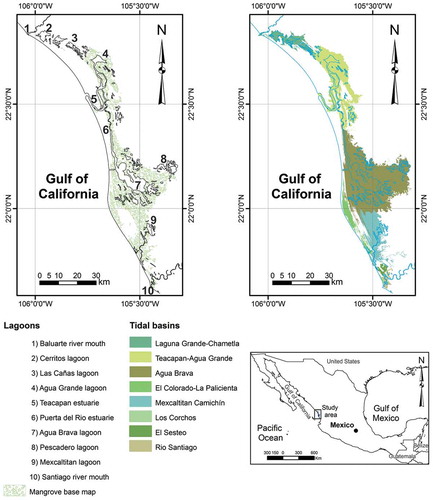
Mangroves are shrub or tree vegetation growing in intertidal zones in tropical and subtropical coasts. They are adapted to highly variable conditions in salinity, tides, winds, temperature and soils (Kathiresan and Bingham 2001). At least five species occur in Mexico, with four of them located in the study area: Avicennia germinans (black mangrove), Laguncularia racemosa (white mangrove), Rhizophora mangle (red mangrove) and Conocarpus erectus (buttonwood). According to the trees’ physiognomy and the local hydrology and topography, the mangrove forests are classified as fringe, riverine and basin forest (Cintron and Schaeffer-Novelli 1985). In the Teacapan-Agua Brava lagoon system, with a mangrove forest of approximately 75,000 ha (Berlanga-Robles and Ruiz-Luna 2007; De la Lanza and Hernández 2017), the basin forest predominates, conformed by patches with dominance of A. germinans in the northern part of the system and by L. racemosa or L. racemosa and R. mangle in the central and southern parts (De la Lanza et al. 1996).

Database integration and preprocessing

The NDVI and EVI data from MODIS/Terra (250 m resolution) were used to evaluate changes in the mangrove canopy of the study area, from 2001 to 2016. The NDVI has been widely used in the study of mangrove cover at different latitudes, but with limitations due to over- or underestimation of the vegetation cover (Rahman et al. 2013). An alternative used to overcome these limitations is the EVI, which is highly sensitive to canopy greenness over dense forests and is resistant to atmospheric haze (Rossi, Rogan, and Schneider 2013). The products MODQ131 V006 used in this study include the two-band version for this index (EVI2), which has been recommended for mangrove assessments because it eliminates noise associated with the subpixel and residual clouds, common in mangrove areas, and because this index is resistant to dark soil background, also common in mangrove areas (Rahman et al. 2013).

The dataset was integrated with 368 HDF files from the global MOD13Q1 V006 data, corresponding to tile h08v06 of the MODIS grid, downloaded from the Land Processes Distributed Active Archive Center (LP DAAC: https://lpdaac.usgs.gov/data_access/data_pool). The 250 m 16 NDVI and 250 m 16 EVI bands were extracted and projected from the MODIS sinusoidal reference system to the UTM system (zone 13N, Datum WGS84) and windowed to fit the study area. The pixel values were rescaled and divided by 10,000 to adjust them to the vegetation index values [0, 1], integrating a 16-day time series from January 2001 to December 2016, from which a monthly time series was produced by averaging images from the same month and year.

Based on previous results from Berlanga-Robles and Ruiz-Luna (2007), non-mangrove areas and mangrove patches ≤ 25 ha were excluded from the analysis, using a raster mask with the results from studies that have provided a baseline for further comparison. Additionally, a climatic database for the study area was downloaded from the National Center for Environmental Prediction (NCEP) – Global Weather Data for SWAT (http://globalweather.tamu.edu/), to trace monthly profiles of the maximum and minimum temperatures, the monthly and accumulated precipitation, relative humidity and solar radiation from April 1999 to July 2014. Finally, a mangrove change from 2005 to 2015 map of the study area was edited from a postclassification comparison of two Mexico´s mangrove distribution maps produced by the National Commission for the Knowledge and Use of Biodiversity (CONABIO), available at http://www.conabio.gob.mx/informacion/gis/. These maps were produced combining unsupervised classifications and visual interpretation of SPOT 5, SPOT 6 and SPOT 7 images, and validated with aerial photographs, reaching overall accuracies of approximately 90% (Rodríguez-Zuñiga et al. 2013; Valderrama-Landeros et al. 2017).

Data analysis

The monthly time series for each vegetation index (NDVI and EVI) were analyzed with a seasonal trend analysis (STA), using the TerrSet 18.30 software (Eastman 2016). The STA involves three stages: first, a harmonic regression was applied to extract five shape parameters of sine waves with an annual and semiannual frequency (Eastman et al. 2009):

$y={\alpha }_0+\sum _{n=1}^{n=2}\left\{a_{n}sin\left(\frac{2\pi nt}{T}\right)+b_n\mathrm{c}\mathrm{o}\mathrm{s}\left(\frac{2\pi nt}{T}\right)\right\}+e\left(Eq.1\right)$

where y is the vegetation index value, t is the time and T is the temporal length of the series; n is a harmonic, e is the error term, and α₀ is the mean of the series. The regression was applied with the first two harmonics on the 12 images by year for the time series to estimate five shape parameters to describe each seasonal cycle: Amplitude 0 (the mean annual signal), Amplitude 1 and Phase 1 (the annual cycle), and Amplitude 2 and Phase 2 (the semiannual cycle). By rearranging the terms after the solution and ignoring the error term, the generalized seasonal curve (Eq. 1) can also be expressed as (Eastman et al. 2009):

$y={\alpha }_0+\sum _{n=1}^{n=2}{a}_{n}sin\left(\frac{2\pi nt}{T}+{\phi }_n\right)\left(Eq.2\right)$

where α_n are the amplitudes, and φ_n are phase angles representing the point of maximum amplitude. The harmonic regressions were achieved at the pixel level, resulting in five shape parameter images for each year. The vegetation phenology cycle inferred from remote sensing data could be characterized by four transition dates: 1) greenup, 2) maturity, 3) senescence and 4) dormancy (Zhang et al. 2003). In the STA analysis with two harmonics, Amplitude 0 represents the vegetation index mean annual signal, whereas Amplitude1 and Phase 1 described the first two dates, and Amplitude 2 and Phase 2 the last two.

In the second stage, the trends over the years in the five harmonic series shape parameters were analyzed with the Theil-Sen median slope. This procedure calculates the slope for each pairwise combination of samples in time, and the median of these slopes is used to characterize the trend. Procedures were also executed at the pixel level, producing a slope image for each of the five shape parameters (Eastman et al. 2009, 2013).

In the third stage, an interactive interpretation of false color composite images was achieved with the Earth Trends Modeler module of TerrSet to translate the trends into fitted seasonal curves for the beginning and the end of the series for different regions. The images produced in the second step were stretched and combined to create false color composite images. The first image was obtained by filtering the slope images of Amplitude 0 in red, Amplitude 1 in green and Amplitude 2 in blue; the second color composite image was produced by filtering slope images of Amplitude 0 in red, Phase 1 in green and Phase 2 in blue. The pixel sets were selected based on the output images to calculate the median slope and intercept values for each of the five shape parameters, using them to fit curves for the beginning and the end of the series for a region in the study area. By plotting these two prototypical curves, changes in seasonality could be determined. Year profiles for the five shape parameters can also be observed with this tool; thus, the interannual variation of the vegetation index can be seen in the profile of the Amplitude 0 (Eastman et al. 2009, 2013; Eastman 2016). We used this tool to extract the adjusted curves of the first and last years of the NDVI and EVI series and the year profiles of Amplitude 0 for each tidal basin.

The climatic variable profiles edited from NCEP data were adjusted with the HarmonicRegression package for R (Westermark 2015) to model:

$y={\alpha }_0+a_{n}sin\left(\frac{2\pi nt}{T}\right)+b_{n}cos\left(\frac{2\pi nt}{T}\right)={\alpha }_0+a_{n}sin\left(\frac{2\pi nt}{T}+{\phi }_n\right)\left(Eq.3\right)$

The correlation between the vegetation index and climatic variable profiles, observed monthly from January 2001 to July 2014, were estimated with the Kendall correlation coefficient, taking into account that the NDVI and climatic variables profiles were not distributed normally. Otherwise, the correlations between the NDVI and EVI fitted curves for each tidal basin and the annual cycle fitted curves for each climatic variable were estimated with the Pearson correlation coefficient.

Additionally, the z values for the Mann-Kendall test for the slopes of five shape parameters were computed at the pixel level, using the Earth Trends Modeler of TerrSet software (Eastman 2016). The z values for the images of Amplitude 0 of both vegetation indices were used to classify the mangrove canopy into three classes, based on the significance level of α = 0.05, with decreasing canopy (z ≤ −1.96), no change in canopy (−196 < z < 1.96), and canopy recovery (z ≥ 1.96). The resulting canopy trend maps were compared with each other and with the 2005–2015 mangrove change map edited from CONABIO maps. The comparisons were made with error matrices (postclassification comparison) to calculate the producer’s accuracy, user’s accuracy, total accuracy and Kappa agreement coefficient (Congalton and Green 1999).

Results

A total mangrove area of approximately 72,680 ha was estimated for the baseline map, covering 45% of the lagoon system. Almost 60% of the mangrove forest was distributed in the Agua Brava tidal basin (AB), while only 0.1% of the forest was found in the Laguna Grande-Chametla basin (LG-C) to the north, and there was no detectable forest in the Los Corchos basin (C). Except for the last two basins, where mangrove cover is not significant at the basin level, mangrove cover was distributed among the remaining six basins, totaling approximately 69,680 ha (96% of the total) if only the ≥ 25 ha patches are considered in the analysis of the NDVI and EVI seasonal trends (Table 1).

Table 1. Mangrove distribution by tidal basin in the Teacapan-Agua Brava lagoon system, Mexico. Basin area estimates are based on Blanco et al. (2011) and mangrove area from a mangrove distribution map by Berlanga-Robles and Ruiz-Luna (2007).

	Basin area (A)		Mangrove area (Ma)			Ma > 25 ha
Tidal basin	ha	%	ha	%	Ma/A	ha	%^2
Laguna Grande-Chametla (LG-C)	10,388	6.4	88	0.1	0.01	0	0
Teacapán-Agua Grande (T-AG)	39,513	24.2	15,938	21.9	0.40	14,994	94.1
Agua Brava (AB)	84,763	52.0	42,281	58.2	0.50	41,450	98.0
El Colorado-La Palicienta (C-P)	6556	4.0	2738	3.8	0.42	2150	78.5
Mexcaltitán-Camichin (M-C)	19,994	12.3	10,869	15.0	0.54	10,444	96.1
Los Corchos (C)	63	0.04	0	0	0.00	0	0
El Sesteo (S)	519	0.3	238	0.3	0.46	156	65.8
Río Santiago (RS)	1313	0.8	525	0.7	0.40	488	92.9
Total	163,106	100.0	72,675	100.0		69,681	95.9

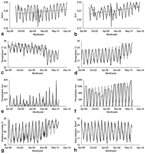
The monthly NDVI and EVI average values oscillated from 0.37 to 0.65 and from 0.18 to 0.33, respectively. In both cases, the minimum values were recorded in December 2007, but they were disregarded because there were no values for the vegetation indices in approximately 90% of the pixels in the study area. The observed monthly profiles from January 2001 to December 2016 displayed similar oscillations (Kendall’s r = 0.75, p = 0), with the maximum values recorded mainly in October-November, while minimums occurred in June-July (Figure 2). Both profiles showed positive monotonic trends, with the NDVI series outputting values of Kendall’s Tau t = 0.158 (p = 0.0012) and Sen’s slope Qi = 0.0003 NDVI/month. The same parameters were assessed for the EVI series output, with t = 0.3 (p < 0.0001) and Qi = 0.0002 EVI/month. In addition, both profiles were significantly correlated in terms of the maximum temperature, accumulated precipitation and solar radiation profiles (Table 2); however, the correlation values were low, and their significance (p < 0.0001) was due to the sample size (n = 163) more than to the relationship among variables (Wheater and Cook 2000).

Table 2. Kendall correlation between the observed NDVI and EVI monthly profiles and the observed profiles of six climatic variables: IV) vegetation index; Tmax) maximum temperature; Tmin) minimum temperature; Ptmon) monthly precipitation; Pacu) accumulated precipitation: Rh) relative humidity; Sr) solar radiation. The correlations were based on 163 months, from January 2001 to July 2014. The bold values are the significant correlations for α = 0.05 and n = 163. In parentheses the p-values.

IV	Tmax	Tmin	Ptmon	Pacu	Rh	Sr
NDVI	−0.29 (< 0.0001)	−0.08 (0.113)	0.06 (0.264)	0.49 (< 0.0001)	−0.01 (0.880)	−0.63 (< 0.0001)
EVI	−0.31 (< 0.0001)	−0.07 (0.172)	0.01 (0.860)	0.47 (< 0.0001)	0.04 (0.580)	−0.48 (< 0.0001)

Figure 2. Vegetation indices and climatic variables profiles: a) NDVI, b) EVI, c) maximum temperature, d) minimum temperature, e) monthly precipitation, f) accumulated precipitation, g) relative humidity and h) solar radiation. solid lines show the observed profiles. dashed lines show the monotonic trend or the fitted seasonal curves.

Trends for the five shape parameters of the NDVI and EVI series were similar, mainly in Amplitude 0, but even so, the EVI seems to be more sensitive in detecting changes in the annual and semiannual cycles. False color composite images for amplitudes and phases of this index showed a more heterogeneous pattern with respect to the composite images of NDVI (Figure 3, available in color in the online digital version).

Figure 3. False color composition images of the slopes of the shape parameters of the NDVI and EVI time series. the images a and b were edited filtering the amplitude 0 slopes in red, the amplitude 1 slopes in green and the amplitude 2 slopes in blue. the images c and d filtered the amplitude 0 slopes in red, the phase 1 slopes in green and the phase 2 slopes in blue. the graphs present the fitted seasonal curves for the beginning (solid) and the end (dashed) of the series for different pixel samples in the study area.

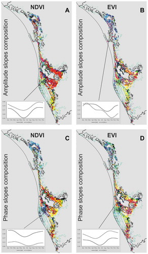
The false color composite images for the amplitudes and phases are shown in red, yellow or magenta; the zones where the Amplitude 0 slopes displayed a significant positive trend were associated with mangroves that have the most closed canopies at the end of the study period. These mangrove patches were mainly concentrated in the Agua Brava tidal basin. Conversely, the zones where the Amplitude 0 slopes had a negative or no trend (seen as green, cyan, blue or black) were associated with mangroves showing open or stable canopies during the study period. These mangroves were mainly in the Teacapan-Agua Grande basin (Figure 3).

Regarding other amplitudes and phases, the composite images shown in yellow, cyan and green were the zones where the Amplitude 1 or Phase 1 slopes had a significant positive trend, and images in magenta, cyan and blue were the zones with positive trends for Amplitude 2 or Phase 2. The white and light gray colors correspond to areas with positive trends for the slopes of the three shape parameters mapped (Amplitude 0-Amplitude 1-Amplitude 2 or Amplitude 0-Phase 1-Phase 2), and the black and dark gray areas correspond to negative or no trends (Figure 3).

In general, the seasonal fitted curves from the beginning (2001) and the end (2016) for the NDVI and EVI series were similar, except the curves of the T-AG and C-P basins, where the minimum values (dormancy) occurred in the late spring, corresponding to the driest period of the year, whereas the highest peaks (maturity) were present in autumn, at the end of the rainy season. Likewise, the curves of 2016 were above those of 2001, indicating the most closed mangrove canopies at the end of the analyzed period, but again, there were exceptions in the T-AG and C-P basins (Figure 4).

Figure 4. Fitted seasonal curves at the beginning (2001) and the end (2016) of the NDVI (left) and EVI (right) times series for tidal basins in the Teacapan-Agua Brava lagoon system: T-AG. Teacapan-Agua Grande; AB. Agua Brava; C-P. El Colorado – La Palicienta; M-C. Mexcaltitan-Camichin; S. El Sesteo; RS. Rio Santiago.

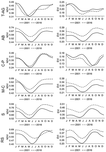
The climatic variables most correlated with the NDVI and EVI fitted curves were the accumulated precipitation (positive) and solar radiation (negative). The EVI curves for the T-AG basin were significantly correlated with all climatic variables, except solar radiation. In some cases, changes in the phases of the vegetation cycles modified the relation with the climatic variables, as correlations were only significant in one year, e.g., the maximum temperature was correlated with the NDVI fitted curve of 2001 but not with the curve of 2016 (Table 3). This result was more common with the EVI fitted curves.

Table 3. Pearson correlation between the NDVI and EVI seasonal fitted curves for the beginning (2011) and end (2016) of the time series with the seasonal fitted curves of six climatic variables. The bold values are the significant correlations for α = 0.05 and n = 12. In parentheses the p-values.

			NDVI					EVI
Basin	Year	Tmax	Tmin	Ptmon	Pacu	Rh	Sr	Tmax	Tmin	Ptmon	Pacu	Rh	Sr
T-AG	2001	−0.54 (0.072)	−0.26 (0.416)	−0.11 (0.742)	0.90 (0.000)	−0.19 (0.561)	−0.90 (0.000)	−0.89 (0.000)	−0.92 (< 0.0001)	−0.89 (0.000)	0.41 (0.184)	−0.91 (< 0.0001)	−0.31 (0.332)
	2016	−0.4 (0.171)	−0.17 (0.600)	−0.04 (0.913)	0.77 (0.003)	−0.10 (0.747)	−0.78 (0.003)	−0.88 (0.000)	−0.84 (0.001)	−0.77 (0.003)	0.58 (0.048)	−0.81 (0.001)	−0.50 (0.099)
AB	2001	−0.60 (0.040)	−0.31 (0.323)	−0.16 (0.623)	0.93 (< 0.0001)	−0.24 0.457)	−0.92 (< 0.0001)	−0.52 (0.084)	−0.23 (0.478)	−0.08 (0.804)	0.88 (0.000)	−0.15 (0.634)	−0.88 (0.000)
	2016	−0.49 (0.104)	−0.18 (0.571)	−0.02 (0.945)	0.93 (< 0.0001)	−0.10 (0.747)	−0.94 (< 0.0001)	−0.34 (0.286)	−0.01 (0.984)	0.15 (0.646)	0.86 (0.000)	0.07 (0.825)	−0.89 (0.000)
C-P	2001	−0.22 (0.487)	0.09 (0.770)	0.25 (0.435)	0.82 (0.001)	0.17 (0.599)	−0.86 (0.000)	−0.37 (0.242)	−0.58 (0.049)	−0.66 (0.019)	−0.29 (0.364)	−0.62 (0.032)	0.37 (0.233)
	2016	−0.16 (0.627)	0.17 (0.605)	0.32 (0.309)	0.79 (0.002)	0.24 (0.450)	−0.85 (0.001)	−0.69 (0.014)	−0.71 (0.010)	−0.70 (0.011)	0.25 (0.434)	−0.70 (0.011)	−0.16 (0.612)
M-C	2001	−0.65 (0.021)	−0.39 (0.204)	−0.25 (0.440)	0.91 (< 0.0001)	−0.33 (0.302)	−0.90 (0.000)	−0.58 (0.050)	−0.31 (0.331)	−0.17 (0.606)	0.87 (0.000)	−0.24 (0.456)	−0.86 (0.000)
	2016	−0.38 (0.227)	−0.05 (0.869)	0.11 (0.742)	0.89 (< 0.0001)	0.03 (0.938)	−0.92 (< 0.0001)	−0.34 (0.287)	0.00 (0.989)	0.15 (0.638)	0.87 (0.000)	0.07 (0.818)	−0.90 (< 0.0001)
S	2001	−0.09 (0.784)	0.21 (0.510)	0.36 (0.254)	0.73 (0.007)	0.28 (0.378)	−0.79 (0.002)	0.45 (0.138)	0.67 (0.016)	0.76 (0.004)	0.28 (0.376)	0.71 (0.009)	−0.38 (0.222)
	2016	−0.17 (0.591)	0.16 (0.614)	0.32 (0.310)	0.82 (0.001)	0.24 (0.453)	−0.87 (0.000)	0.12 (0.720)	0.43 (0.159)	0.57 (0.052)	0.64 (0.026)	0.50 (0.096)	−0.72 (0.009)
RS	2001	−0.56 (0.61)	−0.26 (0.414)	−0.11 (0.735)	0.91 (< 0.0001)	−0.19 (0.565)	−0.90 (< 0.0001)	−0.19 (0.553)	0.11 (0.731)	0.26 (0.424)	0.76 (0.004)	0.18 (0.572)	−0.80 (0.002)
	2016	−0.93 (< 0.0001)	−078 (0.003)	−0.69 (0.014)	0.77 (0.003)	−0.73 (0.006)	−0.69 (0.012)	−0.56 (0.056)	−0.31 (0.327)	−0.17 (0.599)	0.85 (0.000)	−0.24 (0.446)	−0.84 (0.001)

Notes: T_max) maximum temperature, T_min) minimum temperature, P_mon) monthly precipitation, P_acu) accumulated precipitation, Rh) relative humidity, Sr) solar radiation.

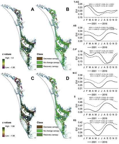
Regarding the NDVI and EVI Amplitude 0 slopes, the z value images were significant at α = 0.05 for 55% and 62% of the pixels, respectively (Figure 5). Based on the output of both indices, the decrease in mangrove canopy was higher in the T-AG basin, with 23% and 34% of the mangrove in this condition. In contrast, mangroves with the highest recovered canopy were present in the AB and S basins, where at least half of the cover showed significant positive trends, and mangroves with decreased canopies were absent in the S basin (Tables 4a and 4b).

Table 4. Mangrove canopy trends and mangrove change. The canopy classes were defined according to the significance (α = 0.05) of Amplitude 0 Z-value images for NDVI (a) and EVI (b). The mangrove change classes (c) were derived from a post-classification comparison of mangrove distribution maps from 2005 and 2015 produced by CONABIO.

a	NDVI
	Decrease canopy		No change canopy				Recovery canopy
Basin	ha	%	ha		%		ha		%	Total
T-AG	3513	23.4	6800		45.4		4681		31.2	14,994
AB	1806	4.4	17,375		41.9		22,269		53.7	41,450
C-P	100	4.7	1638		76.2		413		19.2	2150
M-C	844	8.1	5031		48.2		4569		43.7	10,444
S	0	0.0	50		32.0		106		68.0	156
RS	44	9.0	288		59.0		156		32.1	488
Total	6306	9.1	31,181		44.7		32,194		46.2	69,681
b	EVI
	Decrease canopy		No change canopy				Recovery canopy
Basin	ha	%	ha		%		ha		%	Total
T-AG	5019	33.5	6688		44.6		3288		21.9	14,994
AB	2863	6.9	14,344		34.6		24,244		58.5	41,450
C-P	356	16.6	1413		65.7		381		17.7	2150
M-C	944	9.0	3644		34.9		5856		56.1	10,444
S	0	0.0	44		28.0		113		72.0	156
RS	38	7.7	225		46.2		225		46.2	488
Total	9219	13.2	26,356		37.8		34,106		48.9	69,681
c	2005–2015 mangrove change
	Loss	No change		Gain		Total 2005		Total 2015			Δ
Basin	ha	ha		ha		ha		ha			%
LG-C	69	163		19		231		181			−2.4
T-AG	994	13,119		1581		14,113		14,700			0.4
AB	2406	39,675		300		42,081		39,975			−0.5
C-P	763	2038		56		2800		2094			−2.8
M-C	1031	9694		394		10,725		10,088			−0.6
S	6	194		50		200		244			2.0
RS	56	338		56		394		394			0.0
Total	5325	65,219		2456		70,544		67,675			−0.4
Notes: Δ) Annual average change rate

Notes: Δ) Annual average change rate

Considering the fitted curves and proportion of mangrove canopy conditions by basin, the profiles of the annual averages (Amplitude 0) for both vegetation indices showed significant positive monotonic trends (α = 0.05) in the AB, to the middle of the system, and S and RS basins, to the south. No significant trends were detected for the T-AG (north) and C-P (south) basins, and only a positive trend in the EVI profile was detected for the M-C basin (Figure 5).

Figure 5. z value images and mangrove canopy condition maps generated from the Mann-Kendal significance test for the Amplitude 0 slopes of the NDVI (A and B) and EVI (C and D) time series. The graphs are the NDVI (solid) and EVI (dashed) estimated annual profiles for the tidal basins of the Teacapan-Agua Brava lagoon system. The lines represent the monotonic trend. The t and Qi values are the estimated Mann-Kendal Tau and the Sen slopes (vegetation index/year), respectively.

Additionally, based on the 2005 – 2015 CONABIO mangrove distribution maps, there were approximately 65,219 ha of mangroves without change, 5325 ha were lost, and 2456 ha were gained, resulting in an estimated annual deforestation rate of −0.4%. The highest deforestation rates were recorded in the LG-C and C-P basins, and the highest gains in mangroves were in the AB and S basins. The T-AG basin, identified as the largest mangrove area with canopy decrease, recorded an annual change rate of 0.4% in the postclassification comparison. In the M-C basin, according to the STA results, between 44 to 56% of its mangrove surface registered as recovery canopy, and in comparison with the maps CONABIO presented, the annual change rate was −0.6% (Table 4c).

The results of the analysis for the overall accuracy of the error matrix between the NDVI and EVI canopy trend maps yielded C = 94%, and the Kapa coefficient K’ = 0.9, indicating a perfect agreement between maps, as defined by Landis and Koch (1977). However, only considering the analyzed mangrove area (72,675 ha), the overall accuracy was slightly lower, with C = 86% and K’ = 0.76, which corresponded to substantial agreement (Landis and Koch 1977). The “no change” canopy class obtained the lowest producer´s accuracy, while the “decrease” canopy class obtained the lowest user´s accuracy (Table 5a).

Table 5. Proportional error matrices, based on the 26,097 pixels (163,106.25 ha), comparing of the NDVI and EVI mangrove canopy trends maps (a) and these maps again to a 2005–2015 mangrove change map (b and c).

a)		Canopy trends NDVI map
	Class	0	1	2	3	Total	UA (%)
Canopy trends EVI map	0	0.573	0	0	0	0.573	100.0
	1	0	0.038	0.018	0	0.057	67.6
	2	0	0.001	0.146	0.015	0.162	90.2
	3	0	0	0.027	0.182	0.209	87.2
	Total	0.554	0.039	0.191	0.197	1
	PA (%)	100.0	98.7	76.2	92.2
With background (0): Overall accuracy = 94%, Kappa coefficient = 0.9 Without background (0): Overall accuracy = 86%, Kappa coefficient = 0.76
b)		2005–2015 mangrove change map
	Class	0	A	B	C	Total	UA (%)
Canopy trends NDVI map	0	0.501	0.015	0.049	0.008	0.573	87.5
	1	0.011	0.009	0.017	0.002	0.039	23.3
	2	0.025	0.007	0.155	0.004	0.191	81.1
	3	0.015	0.001	0.180	0.002	0.197	0.8
	Total	0.552	0.033	0.400	0.015	1
	PA (%)	90.7	27.6	38.8	9.9
Overall accuracy = 66%, Kappa coefficient = 0.45
c)		2005–2015 mangrove change map
	Class	0	A	B	C	Total	UA (%)
Canopy trends EVI map	0	0.501	0.015	0.049	0.008	0.573	87.5
	1	0.015	0.012	0.028	0.002	0.057	20.4
	2	0.022	0.005	0.132	0.004	0.162	81.4
	3	0.015	0.001	0.192	0.001	0.209	0.6
	Total	0.552	0.033	0.400	0.015	1
	PA (%)	90.7	35.3	32.9	7.9
Overall accuracy = 64%, Kappa coefficient = 0.43

Notes: 0) background, 1) Decrease canopy, 2) No change canopy, 3) Recovery canopy, A) Mangrove loss, B) Mangrove no change, C) Mangrove gain, PA) Producer accuracy, UA) User accuracy.

The 2005–2015 mangrove change map directly recorded the land-cover changes as a result of postclassification comparison analyses, while the NDVI and EVI canopy trend maps recorded canopy variations that were not always associated with land-cover changes. However, by comparing these maps, high agreement between the classes of mangrove loss with decreasing canopy, the “no change” in mangroves with no change in canopy classes, and the gaining mangrove with canopy recovery classes was expected; but the estimated overall accuracy and Kappa coefficient corresponded to moderate agreement, and the lowest producer´s and user´s accuracies were for the mangrove gain and recovery canopy classes (Tables 5b and 5c).

Discussion

The moderate spatial resolution remote sensing data, such as MODISQ131 products, are inadequate for a reliable and accurate assessment of mangroves found in small patches and narrow strips along rivers (Giri et al. 2015). However, in regionally distributed mangrove forests, containing large patches, the vegetation indices of MODIS with 250 m resolution have allowed the monitoring of these vegetation dynamics (Rogan et al. 2011; Rahman et al. 2013; Rossi, Rogan, and Schneider 2013; Pastor-Guzman, Dash, and Atkinson 2018). The above considerations were imperitive for analyzing the mangrove forest of Teacapan-Agua Brava lagoon; as in agreement with Berlanga (2006), mangrove is distributed in patches averaging 130 ha in size, in a region of 163,000 ha (Blanco et al. 2011).

The minimum patch size of four MOD13Q1 products pixels (250 m each) selected for the study allowed for the analysis of 96% of the total mangrove area previously defined as the baseline map. On this basis, it was possible to characterize the seasonality and trends in mangrove canopies in the study area, and even when it was not possible to detect small gaps in the vegetation patches (Kamal, Phinn, and Johansen 2014), their presence was reflected in the vegetation index values, as a result of the averaged reflectance in the entire pixel (Jiang et al. 2006). In this regard, the use of the EVI has advantages over the NDVI because it is not affected by the presence of soil background effects or saturation due to dense vegetation.

However, we analyzed the mangrove of Teacapan-Agua Brava lagoon system with both vegetation indices, and despite some differences, the results were similar in describing the dominant phenological patterns and monotonic trends, even when the EVI was more sensitive in detecting changes in the amplitude and phase of annual and semiannual cycles. Thus, the false color composites, produced with the shape parameter slope images derived from the NDVI, were more homogeneous than those produced with the EVI. For example, some patches indicating a positive trend for Phase 0 were displayed with some differences in the EVI amplitude trends composite, indicating positive trends also for the Amplitudes 1 or 2, respectively – differences that could be useful for management and restoration purposes. Considering this, Pastor-Guzman, Dash, and Atkinson (2018) found differences between the mangrove phenological variables estimated with four vegetation indices, possibly associated with their sensitivity to different phases of the vegetation growth. Regarding the EVI, they detected more variability in the phenological metrics because it is primarily sensitive to structural proprieties that vary spatially in the canopy.

Although mangroves are perennial, the analysis with both vegetation indices allowed for the identification of phenological (annual) cycles, mostly displaying the maximum greenness in autumn, a few months after the rainy season begins; additionally, the senescence and dormancy were higher to the end of the dry season, when the salinity and evaporation-transpiration deficit reached their maximums in the study area, and producing the highest mangrove litterfall rate (Flores-Verdugo, 1990). This phenological pattern is characteristic for tidal basins with mangrove patches dominated by L. racemosa or mixed patches of L. racemosa and R. mangle (De la Lanza et al. 1996). In the T-AG and C-P basins, where the EVI fitted curves displayed maximum values in winter, the dominance of A. germinans could be the reason for differences in the seasonal pattern.

With regard to climate variables, the maximum temperature, accumulated precipitation and solar radiation output the highest correlations for the two vegetation indices with the observed profiles (from 2001 to 2014), as well as the fitted seasonal curves, at the beginning (2001) and at the end (2016) of the time series. In the tidal basins dominated by L. racemosa or L. racemosa and R. mangle, the seasonal fitted curves of both vegetation indices were positively correlated with the accumulated precipitation, but in the tidal basin dominated by A. germinans, the fitted curves of EVI were negatively correlated with the monthly precipitation and relative humidity. These correlations could be the result of the adaptation of L. racemosa and R. mangle to maximize production under conditions of saturated water supply, as proposed by Miller (1972); whereas A. germinans is adapted to maximize production in drier conditions. In addition, the highest rates of leaf bud and literfall are associated with changes in temperature (Mehlig 2006; Bernini and Rezende 2010), but this factor seems to have a greater influence on the phenology of A. germinans than other species.

As found by Zhang et al. (2014), mangrove litterfall is mostly related to temperature, and it is a common pattern for mangroves to produce approximately 85% of litterfall in the warmest months, with some influence from precipitation and solar radiation. Similarly, Pastor-Guzman, Dash, and Atkinson (2018) found a strong positive correlation between litterfall and temperature in mangroves of Yucatan, Mexico, where mangrove species are the same as in the Teacapan-Agua Brava system. Additionally, these authors reported a weak correlation between litterfall and precipitation, similar to the present findings; however, they found a large negative correlation of the cumulative precipitation with the start of the growing season and the maximum vegetation greenness, indicating that mangroves do not respond immediately to precipitation. Although the beginning of the rainy season stimulates the formation of new leaves (Baserra and Galvani 2013), the closest canopy occurs three to four months later, when they reach their maximum size. This biological process could explain the weak correlations of the observed profiles and fitted seasonal curves of the vegetation indices with monthly precipitation, and the strong positive correlation with the accumulative precipitation detected in this study.

Seasonality in litterfall could also be influenced by solar radiation, producing peaks in the months of highest radiation (Bernini and Rezende 2010; Sharma et al. 2012). This could happen in the study area, mainly during May and June, when according to the seasonal patterns, the mangrove canopy is in a dormant state. Additionally, in these months the driest time occurs, and the photosynthetic activity of the mangroves requires a conservative use of water. Thus, high solar radiation induces an increase in the temperature of the leaves, beyond the acceptable physiological limits and accelerating their fall (Ball and Passioura 1995).

Compared with the last quarter of the 20th century, the Teacapan-Agua Brava lagoon system has reduced the mangrove average annual deforestation, from 0.64% (Berlanga-Robles and Ruiz-Luna 2007; De la Lanza and Hernández 2017) to −0.4% for the 2005–2015 period. Such a reduction is important regarding the condition of the whole system; however, our current approach also allows for the detection of mangrove degradation at the basin level, which was observed in five of the six analyzed basins.

The T-AG basin shows the largest proportion of perturbed mangrove, reaching up to one-third of its area with significant decreasing canopy. Most of the decline is attributed to the reduction of tidal flow and range (Blanco et al. 2011). In other tidal basins, the proportion of degraded mangroves was lower, compared with the mangroves with no change in canopy or recovery canopy; however, in the AB and M-C basins, the mangroves with decreasing canopy were localized in subbasins with hydrological changes, such as flow sequestration, hydrological flow increasing and blocked tidal flow, producing massive mangrove mortality (Blanco et al. 2011).

Although there is not enough evidence, considering that only De la Lanzaet al. (1996) have proposed a rough mangrove distribution species for this wetland complex, the present results could support possible changes in the structure of the mangrove forests, that must be proven. As suggested by the above authors, A. germinans is dominant to the north of the complex, where the tidal basin T-AG displayed a seasonal trend very different to the others, with a maximum amplitude of both vegetation indices in winter. Unfortunately, field data on mangrove structure is not available for the whole study area, but field work data (unpublished data by the authors) confirms that mangroves in this location are practically monospecific for A. germinans. Further confirmation of this, in addition to analytical methods similar to those used in the present study, could help to detect possible changes in mangrove forest structure, as a consequence of different drivers, including climate change. Additionally, regarding the mangrove degradation indicators, the CONABIO data used here indicate that mangrove deforestation in the study area continues, but at rates lower than those recorded at the end of the last century.

Despite the fact that STA and postclassificatory comparison are two different strategies to detect mangrove changes, a higher agreement between results from both analyses was expected, particularly in describing the degradation or recovery patterns in each tidal basin. However, there were coincidences only in two of the six basins analyzed. Part of the disagreement could be attributed to the quantity and location differences found between the baseline map of this study and the 2005–2015 mangrove change map derived from the CONABIO layers. There was a difference of approximately 3000 ha in the mangrove surface estimated between both maps, and almost 10% of the pixels classified as background in the baseline map were classified as a mangrove change class in the 2005–2015 mangrove change map. The interceptions mangrove loss-recovery canopy and mangrove gain-decrease canopy detected in the error matrices are of special interest because these “extreme” disagreements could indicate commission errors in the mangrove change map (reference map), which could explain how 600 to 1000 mangrove hectares were classified as other systems in the CONABIO maps.

Finally, these results highlight that despite the signs of degradation observed in mangroves of the Teacapan-Agua Brava lagoon system, the NDVI and EVI profiles for the whole system and for most of the tidal basins showed positive trends. Almost half of the mangrove forest displayed canopy recovery, and at least one-third of this cover remained without canopy changes. The resistant and resilient mangrove patches were dominated by L. racemosa, and some of them were localized in tidal subbasins with impacts on the river flows and tidal patterns. This could indicate that A. germinans is more vulnerable to changes in these variables than other monospecific or mixed mangrove forests in the study area.

Conclusion

The spatial properties of mangrove forests in the Teacapan-Agua Brava lagoon system, consisting of large patches and wide regional distribution, allow for the use of MOD13Q1 imagery to study their condition, through the analysis of their reflectance properties. Despite the pixel size (250 m), it was possible to analyze 93% of the total mangrove area estimated for the beginning of this century. Additionally, the regularity of data acquisition allowed the performance of a seasonal analysis of the mangrove canopy, limited to other satellite platforms.

The seasonal trend approach, using NDVI and EVI series, output similar phenological patterns and change trends, although the EVI seems to be more sensitive to changes in the semiannual cycles. Additionally, the identification of an annual phenological cycle for mangrove canopies was possible, with the greenest and densest canopy in the early autumn, at the end of the rainy season, and the increasingly open canopies in late spring, in the dry season. This phenological pattern is even more evident when analyzed at the tidal basin level, with mangroves dominated by L. racemosa or mixed L. racemosa and R. mangle patches. However, this slightly differs in tidal basins dominated by A. germinans, where peaks occur in winter. If it is verified, it could be used for future analyses of changes in mangrove structure. Additionally, we found that accumulated precipitation and solar radiation are the main climatic drivers in the seasonality of L. racemosa and R. mangle, while the maximum and minimum temperatures and monthly precipitation were the drivers for A. germinans.

Regarding the long-term changes, mangrove degradation signals were identified in the six tidal basins analyzed; however, four of them recorded positive change trends, only displaying seasonal canopy changes or canopy recovery in 87% of the mangroves. These results, together with those of the 2005–2015 postclassificatory comparison analysis, indicate better conditions for mangrove recovery, compared with those present at the end of the last century. Resilient mangroves were distributed in tidal basins dominated by L. racemosa and R. mangle, while the most disturbed mangrove conditions were found in basins dominated by A. germinans.

Acknowledgements

The authors thank the National Council of Science and Technology (CONACYT-MEXICO) for supporting the SEP-CONACYT Basic Science Project CB-157533 and for the grant to M.R. Nepita (Num. 748017). The MODQ131 products were retrieved online, from the NASA EOSDIS Land Processes Distributed Active Archive Center (LP DAAC) and the USGS/Earth Resources Observation and Science (EROS) Center. Climate data and the 2005 and 2015 mangrove distribution maps used in this study, were courtesy of the National Center for Environmental Prediction (NCEP) - Global Weather Data for SWAT, and the National Commission for the Knowledge and Use of Biodiversity (CONABIO, Mexico).

Disclosure statement

No potential conflict of interest was reported by the authors.

References

- Alongi, D. M. 2002. “Present State and Future of World’s Mangrove Forests.” Environmental Conservation 23 (3): 331–349. doi:10.1017/S0376892902000231.
- Arief, M. C. W., and A. Itaya. 2017. “A Brief Description of Recovery Process of Coastal Vegetation after Tsunami: A Google Earth Time-Series Remote Sensing Data.” Journal Manajemen Hutan Tropika 23 (2): 81–89. doi:10.7226/jtfm.23.2.81.
- Ball, M. C., and J. B. Passioura. 1995. “Mangrove Gain in Relation to Wáter Use: Photosynthesis in Mangroves.” Ecophysiology of Photosynthesis edited by E. D. Schulze and M. M. Caldwell 247–259. Berlin: Springer. . 10.1007/978-3-642-79354-7_12.
- Baserra, L. N. G., and E. Galvani. 2013. “Mangrove Microclimate: A Case Study from Southeastern Brazil.” Earth Interactions 17 (2): 1–16. doi:10.1175/2012EI000464.1.
- Berlanga, R. C. A. 2006. “Characterization of the Coastal Landscapes of Sinaloa and North of Nayarit, Mexico through the Analysis of Land Cover Patterns. [Caracterización De Los Paisajes Costeros De Sinaloa Y Norte De Nayarit, México a Través Del Análisis De Los Patrones De Cobertura Del Terreno].” PhD Diss. Universidad Nacional Autónoma de México, México. 204 p.
- Berlanga-Robles, C. A., and A. Ruiz-Luna. 2002. “Land Use Mapping and Change Detection in the Coastal Zone of Northwest Mexico Using Remote Sensing Techniques.” Journal of Coastal Research 18 (3): 514–522. ORCID: 0000-0001-6878-0929.
- Berlanga-Robles, C. A., and A. Ruiz-Luna. 2007. “Analysis of change trends of the mangrove forest in Teacapan-Agua Brava lagoon system, Mexico. An approximation using Landsat satellite images [Análisis de las tendencias de cambio del bosque de mangle del sistema lagunar Teacapán-Agua Brava, México. Una aproximación con el uso de imágenes de satélite Landsat].” Universidad y Ciencia 23 (1): 29–46.
- Bernini, E., and C. E. Rezende. 2010. “Litterfall in Mangroves in Southeast Brazil.” Pan-American Journal of Aquatic Sciences 5 (4): 508–519.
- Blanco, C. M., F. Flores, M. A. Ortiz, G. De la Lanza, J. Lopez-Portillo, I. Valdéz, C. Agraz, et al. 2011. Diagnostico Funcional De Marismas Nacionales [Functional Diagnosis of Marismas Nacionales. México: Universidad Autónoma de Nayarit, Comisión Nacional Forestal.
- Chen, B., X. Xiao, X. Li, L. Pan, R. Doughty, J. Ma, J. Dong, et al. 2017. “A Mangrove Forest Map of China in 2015: Analysis of Time Series Landsat 7/8 and Sentinel-1A Imagery in Google Earth Engine Cloud Computing Platform.” ISPRS Journal of Photogrammetry and Remote Sensing 131 :104–120. doi:10.1016/j.isprsjprs.2017.07.011.
- Chétet, V., and J. P. Denux. 2011. “Analysis of MODIS NDVI Time Series to Calculate Indicators of Mediterranean Forest Fire Susceptibility.” GIScience & Remote Sensing 48 (2): 171–194. doi:10.2747/1548-1603.48.2.171.
- Cintron, G., and Y. Schaeffer-Novelli. 1985. “Características y desarrollo estructural de los manglares de Norte y Sur América.” Ciencia Interamericana 25 (1–4): 4–15.
- Congalton, R. G., and K. Green. 1999. Assessing the Accuracy of Remote Sensed Data: Principles and Practices.” Boca Raton: Lewis Publishers.
- De la Lanza, E. G., and S. Hernández. 2017. “Natural and Induced Space/Time Environmental Changes in the Teacapán-Agua Brava Lagoon System, NW Mexico.” Journal of Aquaculture & Marine Biology 5 (6): 00140.
- De la Lanza, E. G., S. Sánchez, V. Sorani, and T. Bojórquez. 1996. “Geological, Hydrological, and Mangrove Features in the Coastal Plain of Nayarit, Mexico. [Características Geológicas, Hidrológicas, Y Del Manglar En La Planicie Costera De Nayarit, México].” Boletín de Investigaciones Geográficas 32: 33–54.
- Eastman, J. R. 2016. “TerrSet. Geospatial Monitoring and Modelling System. Tutorial.” Massachusetts: Clark Labs.
- Eastman, J. R., F. Sangermano, B. Ghimire, H. L. Zhu, H. Chen, N. Neeti, Y. M. Cai, et al. 2009. “Seasonal Trend Analysis of Images Time Series.” International Journal of Remote Sensing 30 (10): 2721–2726. doi:10.1080/01431160902755338.
- Eastman, J. R., F. Sangermano, E. A. Machado, J. Rogan, and A. Anyamba. 2013. “Global Trends in Seasonality of Normalized Difference Vegetation Index (NDVI), 1982-2011.” Remote Sensing 5 (10): 4799–4818. doi:10.3390/rs5104799.
- Flores-Verdugo, F., F. González-Farías, O. Ramírez-Flores, F. Amezcua-Linares, A. Yañeez-Arancibia, M. Alvarez, and J. W. Day. 1990. “Mangrove, Aquatic Primary Productivity, and Fish Community Dynamics in Teacapán-Agua Brava Lagoon-Estuarine System (Mexican Pacific).” Estuaries 13: 219–230. doi:10.2307/1351591.
- Friess, D. A., and E. L. Webb. 2014. “Variability in Mangrove Change Estimates and Implications for the Assessment of Ecosystem Service Provision.” Global Ecology and Biogeography 23 (7): 715–725. doi:10.1111/geb.12140.
- Giri, C. 2016. “Observation and Monitoring of Mangrove Forests Using Remote Sensing: Opportunities and Challenges.” Remote Sensing 8 (9): 1–8. doi:10.3390/rs8090783.
- Giri, C., E. Ocheieng, L. L. Tieszen, Z. Zhu, A. Singh, T. Loveland, J. Masek, and N. Duke. 2011. “Status and Distribution of Mangrove Forests of the World Using Earth Observation Satellite Data.” Global Ecology and Biogeography 20 (1): 154–159. doi:10.1111/j.1466-8238.2010.00584.x.
- Giri, C., J. Long, S. Abbas, R. M. Murali, F. M. Qamer, B. Pengra, and D. Thau. 2015. “Distribution and Dynamics of Mangrove Forests of South Asia.” Journal Environmental Management 148: 101–111. doi:10.1016/j.jenvman.2014.01.020.
- Hall-Beyer, M. 2003. “Comparison of Single-Year and Multiyear NDVI Time Series Principal Components in Cold Temperate Biomes.” IEEE Transactions on Geoscience and Remote Sensing 41 (11): 1–8. doi:10.1109/TGRS.2003.817274.
- Heumann, B. W. 2011. “Satellite Remote Sensing of Mangrove Forests: Recent Advances and Future Opportunities.” Progress in Physical Geography: Earth and Environment 35 (1): 87–108. doi:10.1177/0309133310385371.
- Jia, M., Z. Wang, L. L., . K. Song, C. Ren, B. Liu, and D. Mao. 2014. “Mapping China’s Mangroves Based on an Object-Oriented Classification of Landsat Imagery.” Wetlands 34 (2): 277–283. doi:10.1007/s13157-013-0449-2.
- Jiang, Z. Y., A. R. Huete, J. Chen, Y. H. Chen, J. Li, G. J. Yan, and X. Y. Zhang. 2006. “Analysis of NDVI and Scaled Difference Vegetation Index Retrieval of Vegetation Fraction.” Remote Sensing of Environment 101 (3): 366–378. doi:10.1016/j.rse.2006.01.003.
- Kamal, M., S. Phinn, and K. Johansen. 2014. “Characterizing the Spatial Structure of Mangrove Features for Optimizing Image-Based Mangrove Mapping.” Remote Sensing 6 (2): 984–1006. doi:10.3390/rs6020984.
- Kathiresan, K., and B. L. Bingham. 2001. “Biology of Mangrove Ecosystem.” Marine Biology 40: 81–251.
- Kovacs, J. M., F. Flores-Verdugo, J. Wang, and L. Aspden. 2004. “Estimating Leaf Area Index of a Degraded Mangrove Forest Using High Spatial Resolution Satellite Data.” Aquatic Botany 80 (1): 13–22. doi:10.1016/j.aquabot.2004.06.001.
- Kovacs, J. M., J. Wang, and F. Flores-Verdugo. 2005. “Mapping Mangrove Leaf Area Index at the Species Level Using IKONOS and LAI-2000 Sensors for the Agua Brava Lagoon, Mexican Pacific.” Estuarine Coastal and Shelf Science 62: 377–384. doi:10.1016/j.ecss.2004.09.027.
- Kovacs, J. M., J. Wang, and M. Blanco-Correa. 2001. “Mapping Disturbances in a Mangrove Forest Using Multi-Date Landsat TM Imagery.” Environmental Management 27 (5): 763–776. doi:10.1007/s002670010186.
- Kovacs, J. M., M. Blanco-Correa, and F. Flores-Verdugo. 2001. “A Logistic Regression Model of Hurricane Impacts in A Mangrove Forest of the Mexican Pacific.” Journal of Coastal Research 17 (1): 30–37. ORCID: 0000-0002-0520-3996.
- Kuenzer, C., A. Bluemel, S. Gebhardt, T. V. Quoc, and S. Dech. 2011. “Remote Sensing of Mangrove Ecosystems: A Review.” Remote Sensing 3: 878–928. doi:10.3390/rs3050878.
- Landis, J. R., and G. G. Koch. 1977. “The Measure of Observer Agreement for Categorical Data.” Biometrics 33 (1): 159–174.
- Langner, A., J. Miettine, and F. Siegert. 2007. “Land Cover Change 2002–2005 in Borneo and the Role of Fire Derived from MODIS Imagery.” Global Change Biology 13 (11): 2329–2340. doi:10.1111/j.1365-2486.2007.01442.x.
- Long, J. B., and C. Giri. 2011. “Mapping the Philippines´ Mangrove Forest Using Landsat Imagery.” Sensors 11 (3): 2972. doi:10.3390/s110302972.
- Mehlig, U. 2006. “Phenology of Red Mangrove, Rhizophora Mangle L, in the Caeté Estuary, Pará, Equatorial Brazil.” Aquatic Botany 84 (2): 158–164. doi:10.1016/j.aquabot.2005.09.007.
- Miller, P. C. 1972. “Bioclimate Leaf Temperature, and Primary Production in Red Mangrove Canopies in South Florida.” Ecology 53 (1): 22–45. doi:10.2307/1935708.
- Nagelkerken, I., S. J. M. Blaber, S. Bouillon, P. Green, M. Haywood, L. G. Kirton, J. O. Meynecke, et al. 2008. “The Habitat Function of Mangroves for Terrestrial and Marine Fauna: A Review.” Aquatic Botany 89 (2): 155–185. doi:10.1016/j.aquabot.2007.12.007.
- Pastor-Guzman, J., J. Dash, and P. Atkinson. 2018. “Remote Sensing of Mangrove Forest Phenology and Its Environmental Drivers.” Remote Sensing of Environment 205: 71–84. doi:10.1016/j.rse.2017.11.009.
- Rahman, A. F., D. Dragoni, K. Didan, A. Barreto, and J. A. Hutabarat. 2013. “Detecting Large Scale Conversion of Mangroves to Aquaculture with Change Point and Mixed-Pixel Analyses of High-Fidelity MODIS Data.” Remote Sensing of Environment 30: 96–107. doi:10.1016/j.rse.2012.11.014.
- Rodríguez-Zuñiga, M. T., C. Troche-Souza, A. D. Márquez-Mendoza, J. D. Vázquez-Balderas, L. Valderrama-Landeros, S. Velázquez-Salazar, M. I. Cruz-López, et al. 2013. “Manglares De México. Extensión, Distribución Y Monitoreo [Mangroves of Mexico. Extension, Distribution and Monitoring].” Mexico: Comisión Nacional para el conocimiento y Uso de la Biodiversidad.
- Rogan, J., L. Schneider, Z. Christman, M. Millones, D. Lawrence, and B. Schmook. 2011. “Hurricane Disturbance Mapping Using MODIS EVI Data in the Southeastern Yucatán, Mexico.” Remote Sensing Letters 2 (3): 259–267. doi:10.1080/01431161.2010.520344.
- Rossi, E., J. Rogan, and L. Schneider. 2013. “Mapping Forest Damage in Northern Nicaragua after Hurricane Felix (2007) Using MODIS Enhanced Vegetation Index Data.” GIScience & Remote Sensing 50 (4): 171–194. doi:10.1080/15481603.2013.820066.
- Ruiz-Luna, A., J. Acosta-Velázquez, and C. A. Berlanga-Robles. 2008. “On the Reliability of the Data of Extent of Mangroves, a Case Study in Mexico.” Ocean and Coastal Management 51 (4): 342–351. doi:10.1016/j.ocecoaman.2007.08.004.
- Sharma, S., A. T. M. R. Hoque, K. Analuddin, and A. Hagihara. 2012. “Litterfall Dynamics in Overcrowded Mangrove Kandelia Obovate (S., L.) Yong Stand over Five Years.” Estuarine, Coastal and Shelf Science 98: 31–41. doi:10.1016/j.ecss.2011.11.012.
- Tuyholske, C. C., Z. Tane, D. Lopez-Carillo, D. Roberts, and S. Cassels. 2017. “Thirty Years of Land Use/Cover Change in the Caribbean: Assessing the Relationship between Urbanization and Mangrove Loss in Roatan, Honduras.” Applied Geography 88: 84–93. doi:10.1016/j.apgeog.2017.08.018.
- Valderrama-Landeros, L., F. Flores-de Santiago, J. M. Kovacs, and F. Flores-Verdugo. 2018. “An Assessment of Commonly Employed Satellite-Based Remote Sensors for Mapping Mangrove Species in Mexico Using an NDVI-based Classification Scheme.” Environmental Monitoring and Assessment 190 (1): 23. doi:10.1007/s10661-017-6399-z.
- Valderrama-Landeros, L. H., M. T. Rodríguez-Zúñiga, and C. Troche-Souza, S. Velázquez-Salazar, S., E. Villeda-Chávez, J. A. Alcántara-Maya, B. Vázquez-Balderas, et al. 2017. “Manglares de México: actualización y exploración de los datos del sistema de monitoreo 1970/1980–2015. [Mangroves of Mexico: Update and exploration of the monitoring data system 1970/1980-2015]”. México: Comisión Nacional para el Conocimiento y Uso de la Biodiversidad
- Vo, Q. T., C. Kuenzer, Q. M. Vo, F. Moder, and N. Oppelt. 2012. “Review of Valuation Methods for Mangrove Ecosystem Services.” Ecological Indicators 23: 431–446. doi:10.1016/j.ecolind.2012.04.022.
- Westermark, P. O. 2015. “Package ‘Harmonicregresion’.” April 1. https://cran.r-project.org/web/packages/HarmonicRegression/HarmonicRegression.pdf
- Wheater, C. P., and P. A. Cook. 2000. Using Statistics to Understand the Environment. New York: Routledge.
- Wilkie, M. L., and S. Fortuna. 2003. “Status and Trends in Mangrove Area Extent Worldwide.” Food and Agriculture Organization of the United Nations, December.http://www.fao.org/docrep/007/j1533e/J1533E00.htm#TopOfPage
- Younes, C. N., K. E. Joyce, and S. W. Maier. 2017. “Monitoring Mangrove Forests: Are Taking Full Advantage of Technology.” International Journal of Applied Earth Observation and Geoinformation 63: 1–14. doi:10.1016/j.jag.2017.07.004.
- Zhang, H., W. Wenping, W. Dong, and S. Liu. 2014. “Seasonal Patterns of Litterfall in Forest Ecosystem Wordwide.” Ecological Complexity 20: 240–247. doi:10.1016/j.ecocom.2014.01.003.
- Zhang, X., M. A. Friedl, C. B. Schaaf, A. H. Strahler, J. Hodges, F. Gao, B. C. Reed, and A. Huete. 2003. “Monitoring Vegetation Phenology Using MODIS.” Remote Sensing of Environment 84 (3): 471–475. doi:10.1016/S0034-4257(02)00135-9.
- Zhang, X., P. M. Treitz, D. Chen, C. Quan, L. Shi, and X. Li. 2017. ““Mapping Mangrove Forest Using Multi-Tidal Remotely-Sensed Data and Decision-Tree-Based Procedure.” International Journal of Applied Earth Observation and Geoinformation.” 62: 201–214. doi:10.1016/j.jag.2017.06.010.
- Zhu, Y. H., K. Liu, L. Liu, S. W. Myint, S. G. Wang, H. X. Liu, and Z. He. 2017. “Exploring the Potential of WorldView-2 Red-Edge Band-Based Vegetation Indices for Estimation of Mangrove Leaf Area Index with Machine Learning Algorithms.” Remote Sensing 9 (10): 1060. doi:10.3390/rs9101060.