Bathymetry retrieval from optical images with spatially distributed support vector machines

Abstract

This paper presents a spatially distributed support vector machine (SVM) system for estimating shallow water bathymetry from optical satellite images. Unlike the traditional global models that make predictions from a unified global model for the entire study area, our system uses locally trained SVMs and spatially weighted votes to make predictions. By using IKONOS-2 multi-spectral image and airborne bathymetric LiDAR water depth samples, we developed a spatially distributed SVM system for bathymetry estimates. The distributed model outperformed the global SVM model in predicting bathymetry from optical satellite images, and it worked well at the scenarios with a low number of training data samples. The experiments showed the localized model reduced the bathymetry estimation error by 60% from RMSE of 1.23 m to 0.48 m. Different from the traditional global model that underestimates water depth near shore and overestimates water depth offshore, the spatially distributed SVM system did not produce regional prediction bias and its prediction residual exhibited a random pattern. Our model worked well even if the sample density was much lower: The model trained with 10% of the samples was still able to obtain similar prediction accuracy as the global SVM model with the full training set.

Keywords:

• bathymetry
• optical images
• support vector machine
• spatially distributed model

1. Introduction

Mapping water depth or bathymetry was a costly and time-consuming work for boat-based bathymetric survey. With the advancing remote sensing technologies, the efficiency of bathymetry mapping has greatly improved. Although airborne bathymetry LiDAR has been recognized the most accurate and efficient way for collecting shallow water bathymetry (Guenther 2007; Gao 2009), satellite-based optical images alternatively can provide a synoptic view of water color in larger areas with higher revisit frequency (Shahbazi, Théau, and Ménard 2014). Empirical models estimate water depth from satellite images with the calibration of a few ground samples. Eugenio, Marcello, and Martin (2015) used a radiative transfer model to map shallow water bathymetry using high-resolution images. The bathymetry maps they derived from WorldView-2 images were compared with acoustic depths, yielding a prediction RMSE of 1.9 m. The Green band and blue band of multispectral images were used for most bathymetry retrieval works. Furthermore, Stumpf, Holderied, and Sinclair (2003) found ratios of the visible spectrum bands could help deal with varying bottom conditions. Hamylton, Hedley, and Beaman (2015) applied the spatial error regression model to address spatial autocorrelation problem of the model residuals. They concluded that the spatial error model significantly outperformed the regular empirical or physical models.

Machine learning algorithms have been implemented for water depth inversion from optical images. Wang et al. (2007) used a three-layer Back Propagation Neural Network (BPNN) on water depth estimation from Landsat 5 images. They reported that the BPNN model could predict the water depth at a mean absolute error of 0.9 m. They also found the accuracy of the model varied with water depth, from 0.6 m at depth of 0 ~ 5 m to 1.7 m at depth over 10 m. Given that the average water depth in their study area was 5.48 m and the mean absolute error was 0.9 m, the error was significant. Mohamed et al. (2016) used ensemble boosting machine learning algorithm to estimate bathymetry in El-Burullus Lake from a SPOT satellite image. The reference bathymetry data were obtained from echo sounding. They claimed that the least square boosting ensemble method could yield an accuracy of 0.15 m. Their work showed that machine-learning algorithms could replace the traditional multivariate regressive inversion models with better prediction accuracy. Liu et al. (2015) compared the performance of two neural network models: Multilayer Perceptron (MLP) and General Regression Neural Network (GRNN) on bathymetry mapping. They reported that the GRNN had a better root-mean-squared error (RMSE) than the MLP neural network. Kibele and Shears (2016) used the k-nearest neighbor (KNN) nonparametric regression model. They found KNN had a much better prediction accuracy than the traditional Lyzenga’s model (1978). The KNN model searches for the k nearest neighbors in the image multi-dimension feature space to find relevant training samples for regression. Unlike the traditional regression model, KNN model does not have a strong assumption about the data distribution. Their work was another showcase of the superiority of the non-parametric models.

Gao (2015) tested several machine learning algorithms on shallow water depth inversion in the near shore of Great Lakes and found the Support Vector Machine (SVM) with a Gaussian kernel had the best accuracy among the machine learning algorithms. In fact, SVM has been well received in remote sensing data classification. For example, Wang et al. (2016) compared the maximum likelihood classification and the SVM method. They reported that SVM achieved a better overall accuracy as well as the user’s accuracy for channel bars. Moreira, Teixeira, and Galvão (2015) used SVM to classify saline soils from non-saline soils using Thematic Mapper/Landsat-5, Operational Land Imager/Landsat-8, and Hyperion/EO-1 images in Brazil. The classification accuracy ranged from 0.778–0.842. They found SVM worked better with the narrow-band salinity indices of Hyperion than the broadband Landsat images. Xun and Wang (2015) employed SVM to map salt cedar with QuickBird images using an object-based image classification approach. Although separating salt cedar from other vegetation types was challenging, their hierarchical object-SVM method yielded a classification accuracy of 91% and kappa of 0.9. Rodriguez-Galiano et al. (2012) tested several machine-learning classifiers on their resiliency to data quality problems. They reported that SVM was the most robust classifier to work with data with problems such as noise and insufficient sampling.

In the case study of Gao (2015) using the SVM model to predict water depth along the coast of Great Lakes, the accuracy of the SVM model varied with water depth. The depth-dependent error distribution is an evidence of model heterogeneity in the general geographical analyses. In response to this common problem, we propose to use a spatially distributed SVM ensemble system to replace the traditional global SVM model for water depth inversion. The purpose of the present research is to evaluate whether the localized ensemble SVMs could improve over the traditional boosting or bagging sampling strategy. Recently, localized methods are emerging in remote sensing image processing. For example, Su et al. (2014) used a geographically weighted inversion model to retrieve shallow water bathymetry from optical images. They found that using localized samples could largely improve the model accuracy. Deng and Wu (2013) and Wu, Deng, and Jia (2014) recommended a spatially adaptive endmember selection method for spectral mixture analysis. They found that searching for local endmembers and using distance-weighted average produced adequate accuracy for subpixel mapping. These implementations of the location adaptive samples demonstrated that local adaptive models could be superior alternatives to the existing supervised learning models. In this paper, we illustrate the design of a localized sampling framework for support vector machine models. We also tested the sensitivity of the model to the parameters of tessellation and localization, including the search radius of each SVM model, and the spacing of the SVM sites.

2. The distributed SVM model design and implementation

2.1. Selection of the SVM kernel function

The support vector machine partitions the model feature space by hyperplanes through supervised learning. A non-linear classification problem can be solved by projecting the data to a higher dimension space through a kernel function. The specification of the kernel function is subject to user selection. The work by Gao (2015) showed the Gaussian (or radial basis function (RBF)) kernel had the best performance when predicting the bathymetry in the Great Lakes. Lin and Yan (2016) suggested the RBF kernel was a strongly localized kernel function and should be properly selected to maximize the learning ability and avoid the over-training problem. To determine the best γ value, we tested the γ parameter values ranging from 0.1–100 using the training data from the samples (the rest of the samples were for validation). The SVM model prediction accuracy was then assessed by the validation data. As shown in Table 1, the best accuracy was achieved at γ = 1. Increasing or decreasing it led to higher RMSE. Therefore, given the marginal change of RMSE around γ = 1, the SVM models will be defined on the Gaussian kernel function with γ = 1.

Table 1. Parameter test of the SVM Gaussian kernel function.

γ	RMSE (m)
0.01	1.2868
0.1	1.2559
1	1.2496
10	1.4327
100	1.7850

2.2. Tessellation of the study area

The area was tessellated to evenly distributed model spaces. Each space was occupied by a hexagon to train an SVM. Comparing to other regular tessellation shapes such as squares and triangles, using the hexagon maintains the two important spatial properties defined in Boots, Okabe, and Sugihara (1999): uniform adjacency and constant number of neighbors, despite that most GIS and image processing applications used regular grid cells as their basic spatial units. Each SVM was trained using the neighboring samples defined by a search radius. Between search by fixed number of neighbors and search by fixed radius, we used the latter for this case study because the sampling density is almost uniform within the study area. In a situation if samples are unevenly spaced, we recommend using a number of the nearest neighbors as the default spatial search method because the same search radius could return with some unexpected number of neighbors. For example, in a worst scenario, the number of samples included in the research radius could be zero. To test how the tessellation unit size would affect the model prediction accuracy, we created three different tessellations using hexagon units of 6000 m², 12,000 m² and 24,000 m².

2.3. Spatial search for training data

The geometric centers of the hexagons were the locations for spatial searching to train the SVM models. Each model was trained only using the nearby sample data. Supposedly if the search radius was set to infinity, all SVM models will be the same, and then localization will not make any sense. Therefore, setting an appropriate search radius is the essential design component of the localized SVM model. A short search radius may train a learner good at predicting the local conditions; but there is a risk that the short-distance search does not return sufficient number of samples. Therefore, we required at least 30 samples were included in each SVM. By checking the point density of our data, we found 100 meters was the least search radius to include enough samples for each SVM. There are about 2,300 points allocated for training and our study area is about 3.2 km². If the research radius is 50 m, there are only about 6 points by average for each SVM. Insufficient training data will be of a major concern of the supervised learning models in such a short search radius. Therefore, we set the search radius from minimum 100 m and increase it to 200 m and 300 m, to test the best search radius for training the SVMs. Each collection of the samples returned by the spatial search were fed into an SVM for learning. Because they were locally trained, each local SVM was used to predict water depth for the nearby locations. The number of SVMs in the training/prediction system was determined by the size of the tessellation unit and the total study area. For example, if each tessellation unit was 6,000 m², there were 542 locally trained SVM models in the case study area. Another property of the localized model is, if the study area was extended in the future, none of the existing SVMs will be affected by the changing boundary of the study area. A global model, on the contrary, will have to be recalibrated if more samples are added by the change of study area boundary.

Related to the search radius, the sample density as an important parameter for a sampling design also affects the prediction of SVM. LiDAR offers a much efficient way to survey elevation than traditional methods. It does not only improve the sampling accuracy, but also significantly increase the sampling density. A scanning airborne LiDAR system has its sampling density controlled by the laser pulse frequency, scanning mirror rotation speed, and the altitude of the airplane. The first two factors are dependent on the design of the LiDAR systems. The third factor, flight altitude is determined prior to the flight. Higher altitude flights will generate less sampling density but increase the spatial coverage. It is advantageous to find the optimal balance between sampling density and the spatial coverage for the LiDAR surveys. For example, Wang et al. (2013) found the 5 points/m² was the best sampling density for tree stand characterization. In this research, we also test the impact of sample density to the prediction accuracy of the models. We trained the SVMs defined at the above-mentioned tessellations (e.g. T12000 with a search radius of 100 m) with randomly sampled subsets of a variety of sizes (i.e. from 10% to 90% of the total training data). The model accuracy was evaluated using the same validation set.

2.4. Making predictions by SVM ensembles

Individual SVM is a weak learner because of the limited sample sizes from a local area, but their ensemble could make strong predictions. A common practice in using spatial ensemble is the weighted voting. The weights can address the spatial autocorrelation in the neighborhood of the models. It is a common practice to assign the weights inversely to their distance to the prediction location. We adopted the Gaussian spatial distribution function to calculate the weights. The Gaussian distribution function has a zero mean and standard deviation of 100 m, which matches the average search radius. The result will be the weighted average of the nearby SVM predictions. The advantage of the Gaussian kernel is it does not need a cut-off distance like the functions including spherical, linear, and k-nearest neighbor.

The package “e1071” in the R scripting environment was used for SVM model calibration and prediction. Spatial search and distance-based weight calculation was done in a GIS with Python scripts.

3. Case study data and results

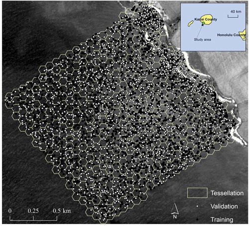
The case study area is located at Waimea Bay – the southwestern shore of Kauai Island of Hawaii, U.S.A (Figure 1). This area is in a moderate tropical climate and known for big-wave surfing activities. Kauai Island water has the most turbidity among all the Hawaiian islands according to the 2014 report by Hawaii Department of Health (2014). The sea floor of the study area is covered by a variety of materials including sand, rock, and pavement inhabited with various amount of macroalgae. An IKONOS-2 image was acquired on 16 February 2006. The image had three visible spectrum ranges – 450–520 nm (blue), 510–600 nm (green), and 630–700 nm (red) and one near-infrared band at 760–850 nm, with a spatial resolution of 4 m. The blue to green spectral range has the best ability to penetrate water because of the combined effects of scattering and absorption in water. Therefore, often were they used to inverse the image colors to depth of water bodies (Jagalingam, Akshaya, and Hegde 2015; Campbell and Wynne 2011, 562). The green band and the blue band were used to train the SVM models in our case study. One of the water column correction methods – deep-water correction (Zoffoli, Frouin, and Kampel 2014; Lyzenga 1978) to obtain the exponential depth dependence X (Lyzenga 1978). The equation is written as:

(1) $X_b=ln\left(L_b-L_{b,\mathrm{\infty }}\right)$(1)

Figure 1. Location of the study area in Kauai County, Hawaii. The tessellation divided the study area into geographical model spaces. Each hexagon had an area of 6000 m². The sample data are split to training (black dots) and validation (white dots) sets. The background image is the green band image of IKONOS with 4 m resolution.

where b is the spectral band, L is the radiance, L_∞ is the deep-water radiance (including scattering). It is worth noting that the deep-water radiance correction also removed the influence of the atmospheric path radiance (Zoffoli, Frouin, and Kampel 2014). We did not conduct any other physically based atmospheric corrections because the atmospheric corrections other than the deep-water radiance subtraction could introduce unwanted artifacts to the data (Monteys et al. 2015). A small portion of deep-water area was used to compute the deep-water radiance of each band, which was subtracted from the image bands. The exponential depth dependence variables (X_b) of the green band and the blue band were used in the SVM model. In 1999, about 4,000 water depth/bathymetry samples of were acquired by the airborne bathymetric LiDAR – Scanning Hydrographic Operational Airborne LiDAR Survey (SHOALS) system. SHOALS system measures both water depth and seabed elevation using its waveform LiDAR with a vertical accuracy of 0.15 m (Irish, McClung, and Lillycrop 2000; Guenther 2007). The maximum water depth of the survey area is about 38 m. The seabed elevation water referenced to the tidal datum at the mean lower low water (MLLW).

In Figure 1, the study site was tessellated to 542 hexagons. Each hexagon was 6,000 m² with a distance to adjacent area center at 100 m. There was one SVM trained at the center of each of the hexagons. The minimum search radius of each SVM model was 100 m. As mentioned in the last section, varying this parameter produced different SVM predictors. The LiDAR sample data were randomly split into two parts: the training set and validation set (Figure 1). The size of the validation set was 1,800. The rest samples of about 2,300 LiDAR points were allocated to the training set. We did not split the data to 80% for training and 20% for testing as used by many other works (e.g. Wang et al. 2016) because our sample data came in with a very high density, thanks to the LiDAR technology. However, adding too much training data not always yields a better model, especially for the non-parametric models. On the other hand, more validation data will bring higher confidence interval for the accuracy assessment. Therefore, we split the data by about 50%-50%, with the training data slightly more than the validation data.

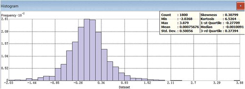
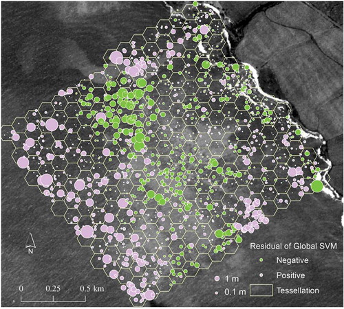
As shown in Figure 1, the distributed SVM system was constructed and used to make predictions by ensemble voting. The model prediction was compared to the validation data. The result showed that the model yielded a good prediction with an RMSE of 0.48 m. This accuracy is much better than the previously reported application of bathymetry retrieval from satellite images (e.g. Gao (2015)). The variogram of the residuals (Figure 2) showed a weak spatial autocorrelation among the residuals. The variogram was fitted using a Stable function: 0*Nugget+1.058* Stable (85.562, 0.592). The range parameter of variogram function was about 86 m, which indicated the residuals at more than 86 m distance apart could be regarded as random. Below the distance of 86 m, there was still some degree of spatial autocorrelation because the SVM models were trained at 100 m search radius. The residual map (Figure 3) of the prediction confirmed the residuals were randomly distributed except those near the coastline and the ledges to the deep water. The normal QQ plot (Figure 4) and histogram (Figure 5) of the residuals also confirmed that the prediction errors almost followed a normal distribution ~(µ = 0,σ = 0.5). A noticeable group of validation points at the south end of the area were out of the model tessellation area, which might be the reason that these points had relatively large errors (about 1.5 m). The outliers in the north section of the coastline might be the result of the inconsistency of the sampling time between the LiDAR data and the IKONOS image. Human activities could be the main reason of bathymetry change during the time gap. Tide height at the time of data acquisition had no impact on the model prediction because the height differences would have been corrected as the bias term in the regression model.

Figure 2. Variogram of the residuals.

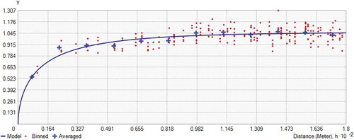
Figure 3. Map of the residuals of the distributed SVM ensemble predictions.

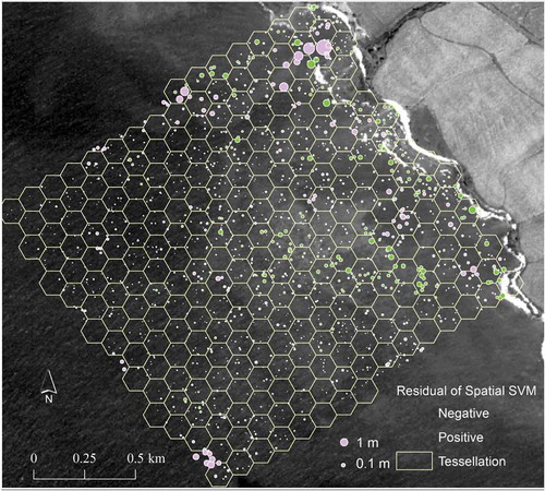
Figure 4. Normal-QQ plot of the residuals.

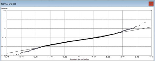
Figure 5. Histogram of the residuals.

4. Discussions

4.1. Problems of the global models

The global SVM model yielded an RMSE of 1.2334 m. As shown in Table 1, tuning the parameter of the SVM kernel function only yielded negligible differences. As shown in Figure 6, the residuals from the global SVM model were generally much larger than that from the distributed SVM ensemble model prediction, and exhibited a strong spatial clustering pattern parallel to the coastline, i.e. underestimated depth in deep water and overestimated in shallow water. The strength of autocorrelation was confirmed by Moran’s I value = 0.22 (p < 0.000001). The similar spatial pattern was reported in many previous research works that tested the global inversion models such as Gao (2015) and Su et al. (2014). The pattern is due to the stationary assumption of the global model, where one model fits all regardless of the complex environment of the study area. A global model can be refined by re-weighting or bagging of the samples Kuncheva (2004), also known as boosting; but none of the existing boosting strategies considers the geographical aspects of the samples.

Figure 6. Residual map of the global SVM model.

Another example of a global model is the ordinary regression inversion model. The optimization target of the model is to minimize the sum of error-squared. Such a model has some strong assumptions like the randomness of residuals. However, most outliers in the model may be due to the complexity of the environment, and can be called environmental outliers. Environmental outliers cannot be treated as data noise but could introduce bias to the models as well. Unless there are sufficient independent variables included in the model, the unexplained variability always exists. Some of the variability is location-dependent because it is from the environment and therefore is called spatial non-stationarity. The non-stationary nature of most models are the defects of the model design. It assumes the model can explain all the variability components of the observations. However, in practice, this assumption is hardly true. The unexplained variability, in our case, resulted from the variable ocean floor cover, turbidity, and bidirectional reflectance distribution function (BRDF) – all could contribute to the satellite image pixel radiance values. Unless all these components are included in the regression equation, the global inversion models are not capable of making reliable predictions. In contrast, the distributed model can overcome the defect of the global models because of the concept of localization. Indeed, the residual map of the distributed SVM model showed the problem has been rectified (Figure 2).

In most remote sensing and environmental studies, the field sample data are always confined by a certain geographic boundary. The global models suffers the modifiable areal unit problem -MAUP (Dark and Bram 2007), i.e. the statistical models trained on the sample data are determined by the arbitrary areal boundary. If the area of interest is expanded or shrunk, the prediction model will have to be recalibrated to fit the new data set. For local models, there will not be such a problem, because expansion or reduction of the study area will only result in addition or removal of individual local SVMs in the prediction system. None of other SVMs will be affected by the changing boundary of the study area.

Our distributed model overcame the problems of a global model and yielded much better predictions. In the following discussions, we will show that a locally trained distributed SVM system can produce a comparable accuracy even the training sample density was only 10% of the original.

4.2. Impact of tessellation

The numbers of SVMs from the three tessellation units (6000, 12,000, and 24,000 m²) were 542, 267, and 132 respectively. For convenience, they were marked as T6000, T12000, and T24000. As shown in Table 2, the best accuracy was achieved by T6000 (0.48 m). However, comparing to T12000, the computation cost of T6000 doubled with a marginal gain in the accuracy (from RMSE 0.50 m to 0.48 m). Therefore, the most cost-effective tessellation would be T12000. Changing the model space (occupied area) would not be a major concern because of its low sensitivity to the model output.

Table 2. Tessellation with different hexagons.

Tessellation	Area (m^2)	Spacing (m)	Number of SVMs	RMSE (m)
T6000	6000	83	542	0.4820
T12000	12000	118	267	0.5004
T24000	24000	166	132	0.5503

4.3. Impact of search radius

The search radius was set to 100 m, 200 m and 300 m to test the sensitivity of the model accuracy. The analysis result showed the best model for each tessellation was the one with the least search radius. However, it was only true by assuming that all search radius settings generate sufficient training samples. We suggested it would be better to keep the search radius as small as possible as long as the number of samples included in the model training is large enough (e.g. 30 points). In addition, it is interesting to see, when the radius was set to 300 m, all three tessellations yielded the similar accuracy (Table 3). Reducing the search radius could increase the model sensitivity to the choice of tessellation unit size. Smaller tessellation unit is more sensitive to the search radius parameter.

Table 3. RMSE of three different tessellations with three different search radius settings.

Search radius (m)	RMSE(T6000)	RMSE(T12000)	RMSE(T24000)
100	0.4820275	0.5004224	0.5503384
200	0.6296925	0.6327278	0.6389739
300	0.7447235	0.7456078	0.7505355

4.4. Impact of sample density

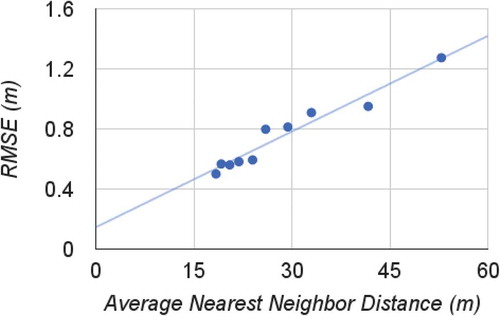
To test the impact of sample density, the training dataset was reduced to its 10% to 90% of its original size by random drawing. The average nearest-neighbor distance, defined as the mean distance of points to their nearest neighbors was used to measure the sample density. The average nearest-neighbor distance tests if a point pattern follows a random Poisson process (Baddeley et al. 2007). If we assume the LiDAR data follow a Poisson distribution because of the randomness of the LiDAR pulse returns, the average nearest-neighbor distance is only associated with point density. We note that the average nearest-neighbor distance can be an index to guide the aerial scanning LiDAR survey instead of the number of points per unit area because it is easy to calculate and has statistical meaning. The test result (Figure 7) showed the model prediction accuracy went down as the sampling density decreased, and the trend line between the RMSE and the average nearest-neighbor distance was almost linear. The gain in accuracy became marginal after the average nearest-neighbor distance went below 24 m. The worst RMSE was in the scenario where the average nearest-neighbor distance is 53 m and only contains about 10% of the original training set. It is interesting that although the sampling density was greatly lowered, the distributed SVM model still produced a comparable accuracy (with RMSE = 1.27 m) to the global model trained with 10 times number of samples (RMSE = 1.23 m). The robustness of SVM to data reduction was also reported in Rodriguez-Galiano and Chica-Rivas (2012). We believe this finding can benefit the works that have difficulty in collecting high-density samples due to the cost or accessibility of the sites: one still can achieve a comparable prediction accuracy from the satellite data using the distributed SVM ensemble model rather than using a global model that requires a much higher sample density.

Figure 7. RMSE by different sample density measured by the average nearest-neighbor distance. The sample dataset with the largest average nearest-neighbor distance (53 m) is a 10% subset of the original sample dataset, followed by 20%, 30%, and so on moving to the shorter average nearest-neighbor distance.

4.5. Comparison with spatially distributed inversion model

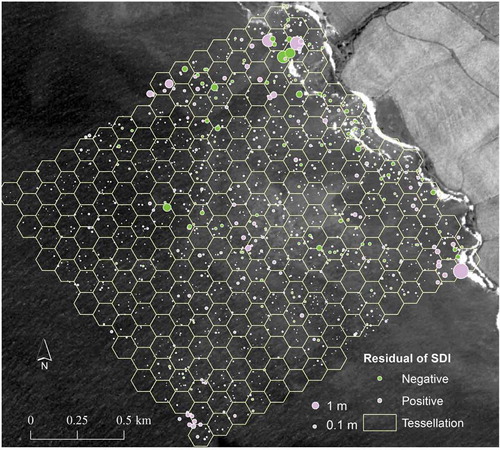
We did a comparison between the distributed SVM ensemble model and the spatially distributed inversion (SDI) model by Su et al. (2014). The residual map (Figure 8) and the RMSE from the SDI model looks similar to our model output. It suggests at the distributed SVM is an alternative to the local adaptive empirical inversion model. In addition, the distributed SVM ensemble approach only used 236 SVMs while the SDI model used almost 2300 regression models to achieve similar accuracy, indicating our model is much more efficient. Furthermore, the SDI model is a linear regression model prone to the uncertainty of many external factors including data noise, the selection of the atmosphere correction model, and the deep-water radiance parameter (Su et al. 2014). Our model uses support vector machines, which are more robust to data noise and other data situations such as low sample density and complex environment (Rodriguez-Galiano et al. 2012). These advantages make the distributed SVM model a better alternative to the SDI model.

Figure 8. Residual map from the Spatially Distributed Inversion Model.

4.6. Comparison with the empirical bayesian kriging interpolation

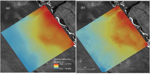
To validate our model prediction with the bathymetry sample data, we compared the rasterized prediction map from our model with the spatial interpolation of the sample data. As shown in Figure 9, the model prediction (Figure 9(a)) agreed with the interpolation (Figure 9(b)) in the overall pattern except some color differences caused by image histogram stretching. It is also apparent that although the spatial interpolation used all the LiDAR samples (4,196 points), the raster data resolution was not as good as the model prediction using the 4 m resolution IKONOS image because spatial interpolation tends to over-smooth the data. This comparison does not only validates our model, but also corroborate one of the advantages of employing satellite images in bathymetry mapping when spatial autocorrelation cannot depict the micro-scale variation in the bathymetry (Su, Liu, and Wu 2015).

Figure 9. Comparison of (a) the SVM model prediction image with (b) the spatial interpolation image using all sample points.

5. Conclusions

In the present research, we designed and tested a distributed SVM ensemble system of using locally trained support vector machines to make an adequate prediction of bathymetry from optical satellite imagery. The localized SVMs and their ensembles outperformed the global SVM model in the prediction accuracy. The distributed SVM model is robust to data reduction. Although higher sampling density could yield better prediction accuracy, the gain of the accuracy was marginal when the average nearest-neighbor distance was shorter than 24 m in a high-density sample design. In addition, our model produced a comparable accuracy only using 10% of the samples to the global model trained with 100% of the samples. When there are limited resources for sampling, using the spatially distributed SVM model could be an effective alternative to the costly efforts of collecting additional samples.

Acknowledgements

This work is partly funded by the College of Humanities & Social Sciences summer stipend program of Louisiana State University and by the National Natural Science Foundation of China (Grant No. 41671095).

Disclosure statement

No potential conflict of interest was reported by the authors.

Additional information

Funding

This work was supported by the National Natural Science Foundation of China [41671095];College of Humanities & Social Sciences summer stipend program of Louisiana State University.

References

- Baddeley, A., I. Bárány, R. Schneider, and W. Weil, eds. 2007. “Spatial Point Processes and Their Applications.” In Stochastic Geometry: Lectures given at the C.I.M.E. Summer School Held in Martina Franca, Italy, 13–18 September 2004, 1–75. Berlin, Heidelberg: Springer Berlin Heidelberg.
- Boots, B., A. Okabe, and K. Sugihara. 1999. “Spatial Tessellations.” In: Geographical Information Systems, P. A. Longley, edited by, Vol. 1, 503–526. New York, NY: John Wiley & Sons.
- Campbell, J. B., and R. H. Wynne. 2011. Introduction to Remote Sensing, 5th ed. New York, NY: Guilford Press.
- Dark, S. J., and D. Bram. 2007. “The Modifiable Areal Unit Problem (MAUP) in Physical Geography.” Progress in Physical Geography 31 (5): 471–479. doi:10.1177/0309133307083294.
- Deng, C., and W. Changshan. 2013. “A Spatially Adaptive Spectral Mixture Analysis for Mapping Subpixel Urban Impervious Surface Distribution.” Remote Sensing Environment 133: 62–70. doi:10.1016/j.rse.2013.02.005.
- Eugenio, F., J. Marcello, and J. Martin. 2015. “High-Resolution Maps of Bathymetry and Benthic Habitats in Shallow-Water Environments Using Multispectral Remote Sensing Imagery.” IEEE Transactions on Geoscience and Remote Sensing 53 (7): 3539–3549. doi:10.1109/tgrs.2014.2377300.
- Gao, J. 2009. “Bathymetric Mapping by Means of Remote Sensing: Methods, Accuracy and Limitations.” Progress in Physical Geography 33 (1): 103–116. doi:10.1177/0309133309105657.
- Gao, S. 2015. “Shallow Water Depth Inversion Based on Data Mining Models.” Master Thesis, Department of Geography & Anthropology, Louisiana State University.
- Guenther, G. C. 2007. “Chapter 8: Airborne Lidar Bathymetry.” In Digital Elevation Model Technologies and Applications: The DEM Users Manual, D. F. Maune, edited by, 2nd ed., 253–320. Asprs Pubns.
- Hamylton, S., J. Hedley, and R. Beaman. 2015. “Derivation of High-Resolution Bathymetry from Multispectral Satellite Imagery: A Comparison of Empirical and Optimisation Methods through Geographical Error Analysis.” Remote Sensing 7 (12): 16257–16273. doi:10.3390/rs71215829.
- Hawaii Department of Health. 2014.“2014 State of Hawaii Water Quality Monitoring and Assessment Report.” The Hawaii Department of Health. http://health.hawaii.gov/cwb/files/2013/05/2014_Draft-Integrated-Report_public-comment.pdf.
- Irish, J. L., J. K. McClung, and W. J. Lillycrop. 2000. “Airborne Lidar Bathymetry: The SHOALS System.” Bulletin of the Permanent International Association of Navigation Congresses 103: 43–53.
- Jagalingam, P., B. J. Akshaya, and A. V. Hegde. 2015. “Bathymetry Mapping Using Landsat 8 Satellite Imagery.” Procedia Engineering 116 (Jan.): 560–566. doi:10.1016/j.proeng.2015.08.326.
- Kibele, J., and N. T. Shears. 2016. “Nonparametric Empirical Depth Regression for Bathymetric Mapping in Coastal Waters.” IEEE Journal of Selected Topics in Applied Earth Observations and Remote Sensing 9 (11): 5130–5138. doi:10.1109/jstars.2016.2598152.
- Kuncheva, L. I. 2004. Combining Pattern Classifiers: Methods and Algorithms. Wiley-Interscience.
- Lin, Z., and L. Yan. 2016. “A Support Vector Machine Classifier Based on A New Kernel Function Model for Hyperspectral Data.” GIScience and Remote Sensing 53 (1): 85–101. Taylor & Francis. doi:10.1080/15481603.2015.1114199.
- Liu, S., Y. Gao, W. Zheng, and L. Xiaolu. 2015. “Performance of Two Neural Network Models in Bathymetry.” Remote Sensing Letters 6 (4): 321–330. doi:10.1080/2150704X.2015.1034885.
- Lyzenga, D. R. 1978. “Passive Remote Sensing Techniques for Mapping Water Depth and Bottom Features.” Applied Optics 17 (3): 379–383. doi:10.1364/AO.17.000379.
- Mohamed, H., A. Negm, M. Zahran, and O. C. Saavedra. 2016. “Bathymetry Determination from High Resolution Satellite Imagery Using Ensemble Learning Algorithms in Shallow Lakes: Case Study El-Burullus Lake.” International Journal of Environmental Science and Development 7 (4): 295. doi:10.7763/IJESD.2016.V7.787.
- Monteys, X., P. Harris, S. Caloca, and C. Cahalane. 2015. “Spatial Prediction of Coastal Bathymetry Based on Multispectral Satellite Imagery and Multibeam Data.” Remote Sensing 7 (10): 13782–13806. doi:10.3390/rs71013782.
- Moreira, L. C. J., A. D. S. Teixeira, and L. S. Galvão. 2015. “Potential of Multispectral and Hyperspectral Data to Detect Saline-Exposed Soils in Brazil.” GIScience and Remote Sensing 52 (4): 416–436. Taylor & Francis. doi:10.1080/15481603.2015.1040227.
- Rodriguez-Galiano, V. F., and M. Chica-Rivas. 2012. “Evaluation of Different Machine Learning Methods for Land Cover Mapping of a Mediterranean Area Using Multi-Seasonal Landsat Images and Digital Terrain Models.” International Journal of Digital Earth 7 (6). doi:10.1080/17538947.2012.748848.
- Shahbazi, M., T. Jérôme, and P. Ménard. 2014. “Recent Applications of Unmanned Aerial Imagery in Natural Resource Management.” GIScience & Remote Sensing 51 (4): 339–365. doi:10.1080/15481603.2014.926650.
- Stumpf, R. P., K. Holderied, and M. Sinclair. 2003. “Determination of Water Depth with High-Resolution Satellite Imagery over Variable Bottom Types.” Limnology and Oceanography 48 (1part2): 547–556. doi:10.4319/lo.2003.48.1_part_2.0547.
- Su, H., H. Liu, L. Wang, A. M. Filippi, W. D. Heyman, and R. A. Beck. 2014. “Geographically Adaptive Inversion Model for Improving Bathymetric Retrieval from Satellite Multispectral Imagery.” IEEE Transactions GIScience and Remote Sensing 52 (1): 465–476. doi:10.1109/tgrs.2013.2241772.
- Su, H., H. Liu, and Q. Wu. 2015. “Prediction of Water Depth from Multispectral Satellite Imagery—The Regression Kriging Alternative.” IEEE Transactions on Geoscience and Remote Sensing 12 (2): 2511–2515. doi:10.1109/LGRS.2015.2489678.
- Wang, C., R. T. Pavlowsky, Q. Huang, and C. Chang. 2016. “Channel Bar Feature Extraction for a Mining-Contaminated River Using High-Spatial Multispectral Remote-Sensing Imagery.” GIScience and Remote Sensing 53 (3): 283–302. Taylor & Francis. doi:10.1080/15481603.2016.1148229.
- Wang, L., A. G. Birt, C. W. Lafon, D. M. Cairns, R. N. Coulson, M. D. Tchakerian, X. Weimin, S. C. Popescu, and J. M. Guldin. 2013. “Computer-Based Synthetic Data to Assess the Tree Delineation Algorithm from Airborne LiDAR Survey.” GeoInformatica 17 (1): 35–61. doi:10.1007/s10707-011-0148-1.
- Wang, Y., P. Zhang, W. Dong, and Y. Zhang. 2007. “Study on Remote Sensing of Water Depths Based on BP Artificial Neural Network.” Marine Science Bulletin 9: 26–35.
- Wu, C., C. Deng, and X. Jia. 2014. “Spatially Constrained Multiple Endmember Spectral Mixture Analysis for Quantifying Subpixel Urban Impervious Surfaces.” IEEE Journal of Selected Topics in Applied Earth Observations and Remote Sensing 7 (6): 1976–1984. doi:10.1109/jstars.2014.2318018.
- Xun, L., and L. Wang. 2015. “An Object-Based SVM Method Incorporating Optimal Segmentation Scale Estimation Using Bhattacharyya Distance for Mapping Salt Cedar (Tamarisk Spp.) With QuickBird Imagery.” GIScience and Remote Sensing 52 (3): 257–273. Taylor & Francis. doi:10.1080/15481603.2015.1026049.
- Zoffoli, M. L., R. Frouin, and M. Kampel. 2014. “Water Column Correction for Coral Reef Studies by Remote Sensing.” Sensors 14 (9): 16881–16931. doi:10.3390/s140916881.