Linking remotely sensed Urban Green Space (UGS) distribution patterns and Socio-Economic Status (SES) - A multi-scale probabilistic analysis based in Mumbai, India

Abstract

Urban Green Spaces (UGS) offer social and environmental benefits that enhance quality of life of the residents. However, due to the underlying social and economic disparities, different sections of urban population have disproportionate level of access to UGS. The environmental inequity owing to the varied UGS distribution poses a challenge to urban planners in efficient resource allocation. This study attempts to counter this challenge using a novel remote sensing-based approach. The variations in UGS distribution (in terms of quantity, quality and accessibility) across the neighbourhoods in Mumbai vis-à-vis the socio-economic status (SES) of neighbourhood residents are assessed using remote sensing-based indicators. Further, as these indicators are susceptible to the effect of changing scales, a multi-scale approach is adopted to study the potential variations in the relationship between SES and spatial metrics of UGS with spatial resolution. The neighbourhood SES was assessed using the newly developed Socio-Economic Status Index (SESI) and the neighbourhoods were classified into multiple SES categories. The UGS were extracted from remotely sensed data using Normalized Difference Vegetation Index (NDVI), and their spatial distribution aspects were characterized using indicators at neighbourhood level. The variations in indicators of UGS distribution in the neighbourhoods belonging to different SES categories were analysed using a logistic regression model. The results showed that, while quantity of UGS is not statistically associated with neighbourhoods SES, the quality and accessibility aspects of UGS share a statistically significant relation with SES. Also, this relation was found to vary significantly with spatial resolutions. Further, it was found that the neighbourhoods with higher SES in Mumbai have a better access to green spaces, indicating spatial inequities in UGS distribution in Mumbai. This study has important implications for planning equitable green spaces in cities that are currently in urbanization transition.

Keywords:

• urban green spaces
• socio-economic status
• spatial metrics
• scale effects
• Mumbai

1. Introduction

Urban green spaces refer to “open spaces situated within city limits with a vegetation cover planted deliberately or inherited from pre-urbanization vegetation left by design or by default” (Lo and Jim 2012). They include parks, gardens, urban forests, and the informal green spaces surrounding defunct industries, railway corridors and historical sites (Gupta et al. 2012). As a key component of urban landscape, green spaces provide ecosystem services, mitigate storm water runoff and pollution, conserve biodiversity, promote social interaction, enhance public health, relieve the citizens from mental and physical stress, and influence property pricings (Franco and Macdonald 2017; De la Barrera et al. 2016a; Gupta et al. 2012). Overall, development of urban green spaces is key for human well-being and sustainability (Badiu et al. 2016). However, the spatial distribution and the distributed effects of urban green spaces are not uniform and are intertwined with the socio-economic milieu. Several studies reported that the affluential neighbourhoods – in terms of income, education, and ethnicity-exhibit more green cover (Pham et al. 2012; Wright Wendel, Zarger, and Mihelcic 2012; Zhou and Kim 2013). On the contrary, the socioeconomically disadvantaged groups are often deprived access to quality green spaces and their associated benefits, which is recognized as an environmental justice issue (Heynen, Perkins, and Roy 2006; Kabisch and Haase 2014; Rigolon, Browning, and Jennings 2018). Such imbalances in spatial distribution of urban green spaces tend to be more severe in developing countries compared to the developed countries (Jim 2013). This deprivation of green spaces is due to general apathy towards planning of green spaces and the conspicuous socio-economic-cultural disparities prevalent in these societies (Wright Wendel, Zarger, and Mihelcic 2012; Senanayake, Welivitiya, and Nadeeka 2013; De la Barrera et al. 2016a). Most research on urban green space and environmental justice are concentrated in developed countries (Kabisch, Qureshi, and Haase 2015; Fernández and Wu 2016), generating a significant blind spot in urban green space studies for cities of developing nations. Yet, the future urbanization will be developing world phenomena (UNPF 2007).

Much of urban growth in developing countries is informal and availability of spatial information on urban green spaces in these cities at neighbourhood level is a challenge. Collecting such information using conventional methods of field surveys and audits is resource intensive and scale limited (Gupta et al. 2012). However, these shortcomings can be overcome with the aid of remote sensing, which provides synoptic and repetitive monitoring of complex urban landscape in a relatively short amount of time (Maktav, Erbek, and Jürgens 2005; Franco and Macdonald 2017). Remote sensing data has been used in various regimes to identify urban green spaces in cities of developing countries (Senanayake, Welivitiya, and Nadeeka 2013; Yao et al. 2014; Zhou et al. 2018). Additionally, it can be used to obtain quantitative measures of configurational aspects of green spaces with the help of spatial metrics (Qian et al. 2015).

Most of the available studies investigating inequities of urban green spaces at neighbourhood level uses measures such as area of green space per inhabitant or percent of green space area (Gascon et al. 2016; De la Barrera, Reyes-Paecke, and Banzhaf 2016b). However, recent studies on this theme recommend adopting an integrated approach that includes quantity, quality and accessibility of urban green spaces (Gupta et al. 2012; Yao et al. 2014; Tian, Jim, and Wang 2014; Haaland and van Den Bosch 2015). It is well recognized that quality and accessibility of green spaces are closely tied to their configurational aspects such as size, shape and aggregation (Jim 2013; Zhou et al. 2018). For example, large green spaces offer scope for more biodiversity, larger social interactions and simultaneous multiple uses. Similarly, elongated and well distributed green spaces have a potential for attracting and benefiting many more residents. Yet only few studies included configurational aspects of green spaces in their assessment of spatial distribution of green spaces across neighbourhoods, particularly for cities in developing countries. For example, De la Barrera, Reyes-Paecke, and Banzhaf (2016b) included spatial metrics related to size, shape and aggregation to assess urban green space distribution across neighbourhoods with different income levels in Santiago, Chile. Li and Liu (2016) and You (2016) used spatial metrics measuring fragmentation as measures of quality of public green spaces in neighbourhoods of Shanghai and Shenzhen, China, respectively. However, these studies mainly relied on very high spatial resolution images (1m or less) acquired from aerial photography or commercial satellites to gather spatial information on urban green spaces.

Urban green spaces in cities of developing countries are vulnerable to the rapid transitions of land use patterns caused by population growth and economic development (Li and Liu 2016; Zhou et al. 2018; Zérah 2007). As a result, these cities require a periodic assessment of green space distribution across neighbourhoods of different socio-economic status to strategize and monitor their greening efforts. The high costs associated with acquiring and processing high spatial resolution images may restrain the local governments from planning green spaces or performing regular green space audits. In this context, satellite images of medium spatial resolution may prove beneficial for these cities as they are often available free of cost. However, the use of medium resolution images for assessing composition and configuration of urban green spaces has limitations. Firstly, smaller patches of urban green spaces often remain undetected (Qian et al. 2015). Secondly, since the landscape patterns are aggregated differently at different spatial resolutions (Walsh et al. 1999; Shen et al. 2004), the spatial metrics assessed from medium resolution images differ from those calculated using high resolution images (Buyantuyev, Wu, and Gries 2010; Oyana, Johnson, and Wang 2014; Feng and Liu 2015). Hence, the resulting relationship between urban green space distribution and neighbourhood socio-economic status may vary with the spatial resolution used. However, examining the potential effects of changing spatial resolution on this relationship is an under-studied area and needs attention. If this context-specific relationship is found analogous across high and medium spatial resolutions, local planners could use low-cost means to undertake periodic green space audits for equitable distribution of its effects.

In this purview, this study attempts to comprehensively analyse the variations in urban green space distribution (in terms of quantity, quality and accessibility) across neighbourhoods of varying socio-economic classes in Mumbai, India, using remote sensing-based spatial metrics derived at multiple spatial resolutions. We chose Mumbai for this study as the city is brimming with urban planning and environmental challenges, in face of proliferating urbanization (Pacione 2006), typical of most cities in developing world.

The novelty of the study is three folds. First, as far as the authors’ knowledge there is no study on the inequities in urban green space distribution across the neighbourhoods of Mumbai. Second, it provides a systematic remote sensing based methodology for assessing the relation between urban green spaces distribution and socio-economic status. Third, a multi-resolution approach is adopted to analyse the hitherto unexplored effect of changing spatial resolution on the relation between socio-economic status and urban green spaces distribution. The primary contribution of the study lies in assessing the imbalances in distribution of green spaces across neighbourhoods with different socio-economic status in Mumbai by harnessing the potential of remote sensing technology. These results might have wider implications on planning of urban green spaces and improving the distributive efficacy.

2. Study area

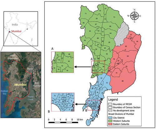
Mumbai is an Indian megacity hosting approximately 12.4 million people (Census PCA 2011) and spread across 458.28 sq km (MCGM 2016). The city is divided into 88 census sections (CS) and is comprised of two revenue districts- Mumbai City and Mumbai Suburban (Figure 1). The Suburban district is further divided into western and eastern suburbs. These suburbs together account for about 75% of the population of Mumbai (Census PCA 2011), and have been a part of the city since the 1950s (Pacione 2006). The civic administration of the city is run by the Municipal Corporation of Greater Mumbai (MCGM), which also carries out the planning of the city by means of the periodical development plans. Although two development plans have been brought out, much of urban development in Mumbai is spontaneous (Pethe et al. 2014) with a mix of residential, commercial and industrial land uses (MCGM 2016).

Figure 1. Geographical location of Mumbai, and map of census sections in Mumbai.Note: Numbers on the map represent the ID of census sections; Insets A and B provide magnified views of census sections.

Mumbai is the financial hub of India (Bardhan et al. 2015a), and the real estate in Mumbai is among the most expensive in the world (Pethe et al. 2014). The city attracts a steady stream of migrants, mostly young single adult males from across the country who mainly come seeking employment with minimal expenditure on accommodation and subsistence (Pacione 2006). However, due to high housing prices, these migrants mostly belonging to economically weaker sections settle in informal settlements like slums (Bardhan et al. 2015a). As a result, about 42% of Mumbai’s population live in slums, which occupy merely 13–15% of the land area (Wurm et al. 2017). These slums mainly lie along creeks, railway lines, peripheries of hills and forests (MCGM 2016). At the intra-city level, the proportion of slum population to the total population is 27.87% and 46.46% for the City and Suburban districts respectively (MCGM 2016), suggesting that the City district has a relatively high socio-economic status vis-à-vis the Suburban district.

Geographically, Mumbai is a peninsula with mangrove forests indenting its eastern and western coastlines. Fishing hamlets dot the entire coast of the city but are mainly concentrated in the north western part of the western suburbs. These hamlets (“Koliwadas”) particularly suffer from a poor standard of civic amenities (Baud et al. 2009). In the northern part of the city lies the Sanjay Gandhi National Park of an area of about 100 sq km. Though the national park is declared to be a no development zone, it is prone to continuous encroachment (Zérah 2007). Also, there are three great lakes in Mumbai- Tulsi, Vihar and Powai; while Tulsi and Vihar lie entirely within the national park, the Powai Lake falls under the census section numbered 85. The city also has a few hillocks and ridges, mostly in the eastern suburbs. Apart from the Sanjay Gandhi National Park and other natural green areas, there are only a few parks and other recreational spaces that constitute the green cover in the city (Zérah 2007).

3. Data and methods

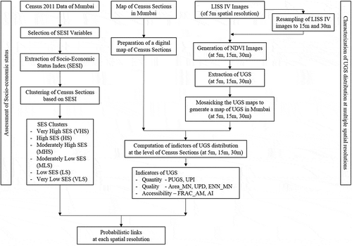
The study workflow adopted to assess the relationship between the socio-economic status (SES) and distribution of urban green spaces (UGS) is given in Figure 2, and involves two main components- (i) assessment of SES, and (ii) characterization of UGS distribution at multiple spatial resolutions. The unit of analysis is “census section,” a territorial unit used for census operations at the intra-city level, and the finest resolution at which the census data is available publicly (Baud et al. 2010). Mumbai is divided into 88 census sections that can be considered as neighbourhoods of the city (Bardhan, Kurisu, and Hanaki 2015b). The data used and detailed methodology of the study are presented in the following sections.

Figure 2. Methodological framework adopted for the study.Note: The numbers represent the ID of the census section; Insets A and B provide magnified views of census sections.

3.1. Data description

Two types of data were used in this study- i) census data- to assess the socio-economic status of Mumbai neighbourhoods, and ii) remote sensing data- to assess the distribution of urban green spaces in Mumbai.

3.1.1. Census data

In this study, the most recent census of India (2011) data (henceforth referred as census 2011) were used to assess the socio-economic status of the census sections in Mumbai. From this data, a set of eleven census variables were used to construct a composite index called Socio-Economic Status Index (SESI) that captures the socio-economic status at census section level (discussed later).

The census 2011 data of Mumbai were obtained in form of two tables, each at the level of census sections. The first table, called the Primary Census Abstract, provides the absolute number of households followed by various demographic data such as number of males, females, literates and working population (Census PCA 2011). The other table, called the “H-Series-Tables on houses, household amenities and assets” (Census HH Amenities 2011), provides data such as the percentages of households availing banking services and owning assets like house and car. In both these tables, for those census sections falling under two MCGM administrative wards, the data of each part are listed separately. A comparison between the two tables revealed that a part of census section number 45 is available in the primary census abstract (represented as 1045) but not in the H-series table. Similarly, an entry numbered 3837 in H-series table is not present in the primary census abstract. Hence, these two entries containing partial census data were ignored for rest of the study (as done in Sidhwani 2015). The remaining data considered for the study, which covers a part of census section 45 and the whole of other eighty seven census sections, account for nearly 98.5% of Mumbai’s population. The population in each census section varied from 3,580 (census section 66) to 814,948 (census section 80).

As the map of census sections in Mumbai in a suitable digital format (viz. “shapefile”) was not available in public domain, we prepared one on a Geographic Information System (GIS) platform. This mapping was based on the census section boundaries given in the maps of assembly constituencies in Mumbai (CEO Maharashtra 2017). The data quality of the digitized map was estimated to have an error of 0.006%± 0.25% at 99% confidence interval.

3.1.2. Remote sensing data

In this study, three IRS Resourcesat-2 Linear Imaging Self Scanner (LISS-IV) images, each covering different parts of Mumbai (path ID-94; row ID- 59; sub scenes- A and C (both acquired on 10 October 2011) and B (acquired on 3 November 2011)), were used. LISS-IV acquires images with a spatial resolution of 5.8m at nadir, and operates in three spectral bands- 0.52–0.59µm, 0.62–0.68µm and 0.77–0.86µm corresponding to the green, red and near infrared wavelengths of electromagnetic spectrum respectively. The three LISS-IV images were obtained from the National Remote Sensing Centre of Indian Space Research Organization as orthorectified geocoded products at a resampled spatial resolution of 5m. The dates of acquisition of these images correspond to the post-monsoon period when the city is lush with green vegetation. Further, to conduct the analysis at multiple spatial resolutions, these three LISS-IV images of 5m spatial resolution were resampled to generate two more sets of images at 15m and 30m resolutions. While 30m corresponds to the spatial resolution of the commonly used Landsat 7 TM images, 15m was chosen to serve as an intermediate resolution for reference. The images were georeferenced and resampled using ERDAS Imagine 2014 package. Thus, a total of nine satellite images, i.e. three for each three spatial resolutions, were used.

3.2. Assessment of socio-economic status

Socio-economic status is multifaceted and has no single direct measure (Kolenikov and Angeles 2009). It is influenced by the local cultural settings in addition to income, education, employment levels of the residents (Bardhan, Kurisu, and Hanaki 2015b). However, resource constraints in developing countries like India limit the scope for an extensive data collection, thus prompting the use of relevant proxy variables to assess various socio-economic status dimensions (Vyas and Kumaranayake 2006).

A newly developed index, called Socio-Economic Status Index (SESI), was used to assess the socio-economic status of Mumbai’s residents at census section level. Conceptually, SESI is similar to the Socio-Economic Cultural Index (SECI) developed for Kolkata city by Bardhan, Kurisu, and Hanaki (2015b) in terms of socio-economic domains chosen in Indian context. However, the domain variables chosen for computing SESI are different considering the spatio-socio-economic contextual differences between Mumbai and Kolkata. The variables for computing SESI were chosen from Census 2011 data primarily, as the census is the primary and only reliable source of statistics on wide ranging demographic, social and economic indicators at intra-city level in India. The domain-specific variables of SESI are as follows:

• Income: Car/Jeep/Van ownership (Car), Availing banking services (Bank), Use of kerosene for lighting (Light_Kero), Use of kerosene as cooking fuel (Fuel_Kero), and House ownership (House).

• Employment: Female working population (FWP) and Total working Population (TWP)

• Education and Culture: Literacy Rate (LR), Average Household Size (AHS), Sex Ratio (SR) and Special Class Population¹ (SCP).

Description of the eleven SESI variables is given in Table 1. Since information on income is not collected in the census, relevant proxy variables in the Indian context such as use of banking services, car ownership, house ownership, use of kerosene as cooking fuel and lighting source were included (Bardhan, Kurisu, and Hanaki 2015b). Sex ratio and female working population were included as gender bias and skewed sex ratio are critical issues in most developing countries. Total working population and literacy rate respectively provide information on the employment and educational profiles of each census section. Average household size was included as it is closely linked with education and wealth; average household size decreases with increase in level of education among women and household wealth status (IIPS 2017). Percentage of special class population was included as they represent the marginalized and historically segregated sections of Indian society (Sidhwani 2015). These variables did not have strong Pearson’s correlation coefficients among them, which makes them suitable to be used for dimension reduction (Su et al. 2014; Li and Liu 2016).

Table 1. Description of the census variables used for computing SESI.

Variable	Description	Mean	Std.Dev.	Minimum	Maximum
Households owning a car/jeep/van (Car)	% of households	15.17	11.41	1.40	53.80
Households availing banking services (Bank)	% of households	88.11	7.27	66.20	98.90
Households using kerosene as the main source of lighting (Light_Kero)	% of households	1.88	1.56	0.10	7.60
Households using kerosene as fuel for cooking (Fuel_Kero)	% of households	13.52	9.45	2.20	39.50
Households owned (House)	% of households	71.41	10.96	38.40	90.50
Female working population (FWP)	% of female population	19.84	5.23	9.06	36.73
Total Working Population (TWP)	% of population	41.99	4.43	35.66	71.09
Literacy Rate (LR)	% of population	82.15	4.70	69.24	90.66
Average Household Size (AHS)	Number of persons per household	4.46	0.32	3.85	5.40
Sex Ratio (SR)	Number of females per 1000 males	856	98.01	329	1022
Special Class Population (SCP)	% of population	6.39	4.32	0.32	21.39

Short form of the variables are given within brackets.

SESI was computed by the weighted aggregation of the eleven extracted variables. The respective weights of the variables for computing SESI were obtained from the first component loading of Principal Component Analysis (PCA). This approach of using PCA first component loading as regression coefficients is widely used in social sciences to derive a unidimensional measure of socio-economic status from a range of correlated multiple variables (Vyas and Kumaranayake 2006). The first component of PCA explains the largest possible amount of variation among the independent variables and is enough to measure socio-economic status (McKenzie 2005; Bardhan, Kurisu, and Hanaki 2015b). For census section “i,” its SESI is given by Equation (1).

(1) $SES{I}_i=W_1\ast Z_{X1}+W_2\ast Z_{X2}+\dots \dots +W_n\ast Z_{Xn}$(1)

where W₁ is the weight assigned to the variable X₁; Z_X1 is the z-score of the variable X₁ for that census section; n is the number of variables.

The resultant SESI scores indicated the socio-economic status of census sections, where higher SESI implied higher socio-economic status. For a better interpretation, the SESI scores were then rescaled from 0 to 100, where 0 and 100 signify the SESI of the lowest- and highest-ranking census sections respectively. Then, based on SESI values, the census sections were then clustered into six categories. The number of clusters was determined using NbClust package in R (Charrad et al. 2015), and clustering was done based on “Partitioning Around the Medoids” method using pam function of cluster package in R (Maechler et al. 2017).

3.3 Characterization of urban green spaces

3.3.1. Extraction of urban green spaces

By definition, urban green spaces include all vegetated open spaces in urban areas irrespective of ownership or access (Lo and Jim 2012; Zhou et al. 2018; Du Toit et al. 2018). In this study, the urban green spaces in Mumbai were extracted from satellite imageries using the Normalized Difference Vegetation Index method (Senanayake, Welivitiya, and Nadeeka 2013). NDVI measures the vegetation intensity in each pixel using the spectral reflectances in the red (R) and near infrared (NIR) bands in form of (NIR-R)/(NIR+ R) (Mennis 2006). It varies from −1 to + 1, and is typically greater than 0.2 for vegetated areas (Franco and Macdonald 2017). In this study the satellite images used cover different parts of Mumbai and were acquired on different dates. Hence, each image was analysed separately and after radiometric correction the corresponding NDVI images were generated. While prior studies (e.g. Senanayake, Welivitiya, and Nadeeka 2013) used visual inspection to choose an optimum NDVI threshold to distinguish green and non-green pixels, in this study the threshold was objectively determined using the Otsu threshold selection method (Otsu 1979). This method uses a criteria function defined by the between-class variance and the total variance, as given in Equation (2).

(2) $\eta \left(T\right)=\frac{{\delta }_b^2}{{\delta }^2}$(2)

where η(T) is the criterion function, ${\delta }_b^2$ is the between-class variance, ${\delta }^2$ is the total variance, and T is the optimum threshold. The criterion function is evaluated for all possible threshold values, and the one that maximizes η(T) is considered to be the optimal threshold (Sunder, Ramsankaran, and Ramakrishnan 2017). Accordingly for each NDVI image an optimal threshold value was computed in MATLAB, and a corresponding binary image comprising vegetation and non-vegetation areas was generated. Subsequently, the three binary images of same spatial resolution were merged to generate the maps of urban green spaces in Mumbai at 5m, 15m and 30m resolutions. These maps include accessible green spaces (such as parks and, gardens) and also inaccessible green spaces (such as urban forests and mangroves).

3.3.2. Indicators for assessing urban green space distribution

As recommended by recent studies (Gupta et al. 2012; Yao et al. 2014; Tian, Jim, and Wang 2014; Haaland and van Den Bosch 2015), this study assessed the distribution of urban green space (UGS) patches among Mumbai’s neighbourhoods by integrating the quantity, quality and accessibility aspects. Quantity of UGS was measured using two commonly used indicators: Percentage of UGS area in a census section (PUGS) and UGS area per inhabitant (UPI) (De la Barrera, Reyes-Paecke, and Banzhaf 2016b; Li and Liu 2016). The quality of green spaces is influenced by their size and fragmentation, wherein larger and connected green patches offer more quality spaces than smaller and fragmented patches (Jim 2013; Tian, Jim, and Wang 2014; Li and Liu 2016; You 2016). Hence, quality of green spaces was assessed using three spatial metrics relevant to size and fragmentation: Mean area of UGS patches (Area_MN), UGS patch density (UPD), and Mean Euclidean nearest neighbour distance of UGS patches (ENN_MN). For accessibility, prior studies generally considered the total population residing in blocks falling within a certain distance from UGS patches (De la Barrera, Reyes-Paecke, and Banzhaf 2016b; Li and Liu 2016; You 2016). However, as the population data of Mumbai is not available at block-level, the accessibility component was assessed in terms of shape and aggregation level of UGS patches. Here, the underlying assumption is that more residents live in proximity to UGS when the green spaces in a census section are more convoluted and disaggregated (Tian, Jim, and Wang 2014; Jim 2013). Accordingly, two spatial metrics were selected as the accessibility indicators: Area-weighted mean fractal dimension index (FRAC_AM) and Aggregation index (AI) of the urban green space patches. Description of all the chosen UGS distribution indicators is provided in Table 2. These indicators were computed separately for each of the three urban green spaces maps having different spatial resolutions. The spatial metrics were obtained at class-level (here, class refers to urban green spaces) for each census section in Mumbai using an eight-cell neighbourhood rule in FRAGSTATS v4.2 (McGarigal, Cushman, and Ene 2012).

Table 2. Description of the urban green space distribution indictors used in the study.

Domain	Indicator	Formula	Description	Units and Range
Quantity	Percentage of UGS area (PUGS)	PUGS = $\frac{A_{UGS}}{A_{CS}}$ * 100	where $A_{UGS}$ is the area of UGS in the census section, and $A_{CS}$is the area of census section.	Percent; 0 ≤ PUGS ≤ 100
	UGS area per inhabitant (UPI)	UPI = $\frac{A_{UGS}}{P_{CS}}$	where $A_{UGS}$ is the area of UGS in the census section, and $P_{CS}$is the population of census section.	m^2 per person; UPI ≥ 0
Quality	Mean area of UGS patches* (Area_MN)	Area_MN = $\frac{A_{UGS}}{n}$	where $A_{UGS}$ is the area of UGS in the census section, n is the number of UGS patches in the census section.	ha; Area_MN ≥ 0
	Urban green space patch density* (UPD)	UPD = $\frac{n}{A_{CS}}$ * 100	where n is the number of UGS patches in the census section, and $A_{CS}$ is the area (in ha) of that census section.	number per 100 ha; PD ≥ 0
	Mean Euclidean nearest neighbour distance of UGS patches* (ENN_MN)	ENN_MN = $\frac{{\sum }_{i=1}^n{d}_i}{n}$	where $d_i$ is the distance between an UGS patch i and its nearest neighbouring patch in the census section, n is the number of UGS patches in the census section.	m; ENN_MN ≥ 0
Accessibility	Area weighted mean fractal dimension index* (FRAC_AM)	FRAC_AM = $\sum _{i=1}^{i=n}\left[\left(\frac{a_i}{A_{UGS}}\right)\left(\frac{2ln0.25p_i}{ln{a}_i}\right)\right]$	where $a_i$ and $p_i$ denote the area and perimeter of an UGS patch i respectively, n is the number of UGS patches in the census section, $A_{UGS}$ is the area of UGS in the census section.	Unitless; 1 ≤ FRAC_AM ≤ 2 FRAC_AM = 1 if the patches are square-shaped. FRAC_AM = 2 if the patches are highly convoluted.
	Aggregation index* (AI)	AI = $\left[\frac{J}{maxJ}\right]\ast 100$	where J is the number of joins between pixels of UGS patches in the census section based on single-count method, max J is the maximum possible value of J.	Percent; 0 ≤ AI ≤ 100 AI = 0 if the patches are maximally disaggregated. AI = 100 if the patches are maximally compact.

*Source: McGarigal (2015).

3.4. Probabilistic analysis between socio-economic status categories and indicators of urban green space distribution

To analyse the variations in urban green space distribution among neighbourhoods having different socio-economic status groups, prior studies used either a simple comparison method (De la Barrera, Reyes-Paecke, and Banzhaf 2016b) or linear regression methods (Li and Liu 2016; You 2016). However, a simple comparison may not reveal the statistical significance of variations in urban green space distribution aspects. Similarly, the linear regression methods assume that urban green space distribution indicators share a linear relation with neighbourhood socio-economic status, thereby concealing potential non-linear relationships. Hence, this study adopted Multinomial Logistic Regression (MLR) models to identify the relationship. MLR is a generalized form of binary logistic regression where the dependent variable can belong to any of multiple categories (Hosmer and Lemeshow 2004). Unlike linear regression, in MLR there is no assumption of linear relationship between the dependent and independent variables (Bewick, Cheek, and Ball 2005).

MLR models predict the relative probability of membership in other categories against a reference category on natural log scale using a linear combination of independent variables. For example, for n independent variables and a dependent variable Y having m possible categories, assuming that the first category is the reference, there would be m-1 MLR models as given in Equation (3):

(3) $ln\frac{p\left(Y=c\right)}{p\left(Y=1\right)}={\beta }_{0c}+{\beta }_{1c}{X}_1+\dots .+{\beta }_{nc}{X}_n$(3)

where c = 2,3…,m; p(Y = c) = probability of membership in category c; p(Y = 1) = probability of membership in the reference category; $p\left(Y=c\right)/p\left(Y=1\right)$ is the relative probability of membership in category c; ${\beta }_{0c}$ is the intercept and ${\beta }_{1c}$…${\beta }_{nc}$ are the regression coefficients for the category c estimated using maximum likelihood method; $X_1$…$X_n$ are the independent variables.

In Equation (3), the regression coefficients associated with each independent variable signify the odds ratio (i.e. the multiplicative factor of change in relative probability) of category c on natural log scale for a unit increase of that variable while other variables remain constant.

In this study, MLR was performed by considering the urban green space distribution indicators derived for a particular spatial resolution as independent variables and the socio-economic status categories as dependent variable, with the lowest socio-economic status as the reference category. Thus, three sets of MLR models were developed for the three spatial resolutions considered. A stepwise backward approach based on Akaike Information Criteria (AIC) was used to build the MLR models using the most informative variables, and the significance level was chosen as 5%. These MLR models were built using multinom function of nnet package in R (Ripley et al. 2017).

4. Results

4.1. Classification of census sections based on socio-economic status

The weights of the eleven SESI variables derived from principal component analysis indicated that SESI is positively related to economic and asset ownership parameters like Bank (0.44) and Car (0.38) and negatively related to poverty indicators like Light_Kero (−0.33) and Fuel_Kero (−0.41). However, the weight of the variable House was found to be only 0.02, suggesting a poor impact of house ownership on socio-economic status in Mumbai. Further, SESI shared positive relationship with the two employment variables- WFP (0.18) and TWP (0.04). With respect to education and culture, SESI showed positive relationship with LR (0.43) and SR (0.24), and a negative relationship with AHS (−0.31) and SCP (−0.15). Hence, a higher SESI did indicate the higher socio-economic status (SES) of the residents.

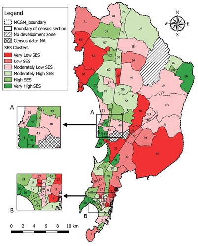
The clustering of census sections in Mumbai based on their SESI scores resulted in 6 clusters. These clusters were ranked in ascending order of their median SESI and were named Very Low SES (VLS), Low SES (LS), Moderately Low SES (MLS), Moderately High SES (MHS), High SES (HS) and Very High SES (VHS) as shown in Table 3. Out of the eighty eight census sections in Mumbai, twenty five belonged to lower socio-economic status categories (i.e. VLS and LS) while twenty six of them fell under higher socio-economic status categories (i.e. HS and VHS); the remaining were associated with moderate socio-economic status categories (i.e. MLS and MHS). The median SESI for the city district, western suburbs and eastern suburbs were found to be 53.67, 52.41 and 41.17 respectively, indicating that the eastern suburbs had a relatively lower socio-economic status at intra-city level.

Table 3. Descriptive statistics of the socio-economic status clusters.

SES Cluster	N	MedianSESI	Std.Dev.	MinimumSESI	MaximumSESI
Very Low SES (VLS)	13	19.08	7.86	0	23.79
Low SES (LS)	12	33.72	3.32	27.74	38.93
Moderately Low SES (MLS)	19	44.96	3.24	39.36	49.56
Moderately High SES (MLS)	18	56.91	3.70	51.32	62.28
High SES (HS)	15	70.61	3.72	65.79	78.07
Very High SES (VHS)	11	88.05	6.17	80.26	100
Total	88	50.44	22.64	0	100

The spatial pattern of socio-economic status of census sections in Mumbai is shown in Figure 3. While the eastern suburbs predominantly had a lower socio-economic status, the city district and the western suburbs showed a medley of different socio-economic status categories. The Koliwadas in the north-western part of the suburbs, the census sections adjacent to the national park and those at the centre of the city were found to have a lower socio-economic status. On the other hand, the census sections in the south-western part of city district and the southern end of western suburbs had a higher socio-economic status.

Figure 3. Socio-economic status clusters of census sections in Mumbai.

4.2. Characterization of urban green spaces at different spatial resolutions

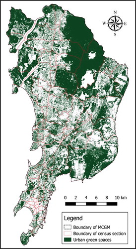
The map of urban green spaces in Mumbai extracted from satellite images at 5m spatial resolution is shown in Figure 4. It is observed that the census sections in the north-western part of western suburbs and those adjoining the Sanjay Gandhi National Park were verdant with compact urban green space patches. The hillocks and mangroves in the eastern suburbs also appeared as composite green blocks. The southern part of the city district, which includes some of the oldest neighbourhoods of Mumbai, appeared to have sparser green cover. Also, the slum neighbourhoods in the city, such as Dharavi (in census section 33), were found to possess little vegetation amidst them.

Figure 4. Map of urban green spaces in Mumbai extracted from satellite images of 5m spatial resolution.

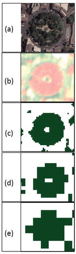
A comparison of urban green space maps extracted from satellite images of different spatial resolutions revealed that at coarser spatial resolutions smaller green space patches remained undetected while larger green spaces grew in size gaining the peripheral non-green cells. This is depicted in Figure 5 with the example of Horniman circle garden, a prominent green space located in South Mumbai. This simultaneous swapping of cells occurring at courser resolutions caused considerable differences among the urban green space distribution patterns assessed at different spatial resolutions. For example, the census section 7 that had sixteen green space patches at 5m resolution was found to have none at 15m and 30m resolutions. Similarly, the census section 10 that had two green space patches at 15m resolution appeared devoid of green spaces at 30m resolution. As a result, changing spatial resolution effected variations in the urban green space distribution indicators assessed at census section level. This is illustrated in Table 4 with the example of census section 1.

Table 4. Urban green space distribution indicators of census section 1 at different spatial resolutions.

SpatialResolution (m)	PUGS	UPI	Area_MN	UPD	ENN_MN	FRAC_AM	AI
5	62.85	21.51	0.77	80.83	14.57	1.39	92.07
15	66.16	22.65	4.19	15.78	36.14	1.33	86.15
30	71.95	24.65	32.58	2.21	71.66	1.28	84.92

Figure 5. Scene covering Horniman Circle Garden, Mumbai.a) Google Earth image; b) Standard false colour composite of LISS IV image (5m); c) UGS map at 5m resolution; d) UGS map at 15m resolution, and e) UGS map at 30m resolution. Note: In panels (c) to (e), the urban green spaces are shown in green.

4.3. Association between socio-economic status and urban green space distribution indicators derived at various spatial resolutions

4.3.1. At 5m spatial resolution

Table 5 gives the result² of multinomial logistic regression associating socio-economic status and the urban green space distribution indicators extracted at 5m spatial resolution, considering VLS category as reference. The results showed that at this resolution Mumbai’s neighbourhoods showed significant variations in green space quality and accessibility but not in terms of quantity. Among the socio-economic categories, only LS, HS and VHS exhibited statistically significant differences in either quality or accessibility compared with VLS. Census sections belonging to LS were found to be statistically associated with high UPD, FRAC_AM and AI values. This indicated that in these sections green spaces were distributed in form of more number of complex-shaped but aggregated patches. Census sections falling in HS and VHS categories were found to have statistically significant relation with high values of FRAC_AM, suggesting these sections had more complex-shaped green spaces.

Table 5. Multinomial Logistic Regression model for socio-economic status and the urban green spaces indicators derived at 5m spatial resolution.

SES Category	Independent Variable	Value	Odds Ratio (OR)	ORLower Bound (95%)	ORUpper Bound(95%)
LS	Intercept	−60.043***
	UPI	0.000	1.000	0.997	1.002
	UPD	0.032***	1.033	1.020	1.045
	FRAC_AM	14.688***	2.392 e + 06	100.456	5.698 e + 10
	AI	0.406***	1.501	1.275	1.767
MLS	Intercept	−1.340
	UPI	−0.013	0.987	0.960	1.016
	UPD	−0.009	0.990	0.978	1.004
	FRAC_AM	3.062	21.364	0.021	2.152 e + 04
	AI	−0.004	0.996	0.909	1.092
MHS	Intercept	−3.406
	UPI	−0.007	0.992	0.969	1.017
	UPD	−0.001	0.999	0.988	1.011
	FRAC_AM	6.247	516.411	0.443	6.013 e + 05
	AI	−0.046	0.955	0.873	1.046
HS	Intercept	−16.822***
	UPI	−0.096	0.909	0.818	1.009
	UPD	0.005	1.005	0.992	1.018
	FRAC_AM	12.571***	2.882 e + 05	340.544	2.439 e + 08
	AI	0.015	1.015	0.877	1.174
VHS	Intercept	−22.336***
	UPI	−0.003	0.997	0.985	1.008
	UPD	0.001	1.001	0.988	1.015
	FRAC_AM	24.906***	6.553 e + 10	2.672 e + 08	1.607 e + 13
	AI	−0.118	0.888	0.779	1.013

Reference Category: VLSAIC: 320.35

**significant at p < 0.05***significant at p < 0.01

4.3.2. At 15m spatial resolution

Table 6 gives the result of multinomial logistic regression associating socio-economic status and the urban green space distribution indicators extracted at 15m spatial resolution, considering VLS category as reference. The results showed that at this resolution Mumbai’s neighbourhoods showed significant variations only in terms of green space quantity. Among the socio-economic categories, only VHS showed statistically significant association with high PUGS. This indicated that at this resolution census sections belonging to VHS category were found to possess more areas under green cover.

Table 6. Multinomial Logistic Regression model for socio-economic status and the urban green spaces indicators derived at 15m spatial resolution.

SES Category	Independent Variable	Value	Odds Ratio (OR)	OR Lower Bound (95%)	OR Upper Bound (95%)
LS	Intercept	−1.668
	PUGS	0.049	1.050	0.997	1.106
	Area_MN	−0.165	0.848	0.658	1.093
MLS	Intercept	0.043
	PUGS	0.017	1.017	0.974	1.062
	Area_MN	−0.139	0.870	0.678	1.118
MHS	Intercept	−0.105
	PUGS	0.024	1.025	0.975	1.077
	Area_MN	−0.320	0.726	0.411	1.282
HS	Intercept	−0.507
	PUGS	0.068	1.070	0.992	1.156
	Area_MN	−1.991	0.136	0.015	1.249
VHS	Intercept	−2.669**
	PUGS	0.095**	1.100	1.011	1.197
	Area_MN	−0.953	0.385	0.110	1.348

Reference Category: VLSAIC: 319.174

**significant at p < 0.05***significant at p < 0.01

4.3.3. At 30m spatial resolution

Table 7 gives the result of multinomial logistic regression associating socio-economic status and the urban green space distribution indicators extracted at 30m spatial resolution, considering VLS category as reference. The results showed that at this resolution Mumbai’s neighbourhoods showed significant variations only in terms of green space accessibility. Among the socio-economic categories, only MLS showed statistically significant association with high AI. This indicated that at this resolution census sections belonging to MLS category were found to possess more aggregated green space patches.

Table 7. Multinomial Logistic Regression model for socio-economic status and the urban green spaces indicators derived at 30m spatial resolution.

SES Category	Independent Variable	Value	Odds Ratio (OR)	OR Lower Bound (95%)	OR Upper Bound (95%)
LS	Intercept	−6.126
	UPI	0.000	1.000	0.996	1.002
	UPD	0.091	1.095	0.971	1.234
	ENN_MN	−0.020	0.980	0.894	1.075
	AI	0.083	1.086	0.994	1.187
MLS	Intercept	−10.514**
	UPI	−0.007	0.993	0.977	1.010
	UPD	0.057	1.059	0.955	1.175
	ENN_MN	0.033	1.033	0.999	1.069
	AI	0.104***	1.110	1.028	1.198
MHS	Intercept	−0.135
	UPI	−0.006	0.994	0.969	1.018
	UPD	0.024	1.024	0.933	1.124
	ENN_MN	−0.002	0.998	0.963	1.034
	AI	0.005	1.005	0.942	1.071
HS	Intercept	7.949
	UPI	−0.110	0.896	0.796	1.008
	UPD	−0.050	0.951	0.859	1.053
	ENN_MN	−0.049	0.952	0.904	1.003
	AI	−0.025	0.975	0.905	1.050
VHS	Intercept	8.704
	UPI	−0.005	0.994	0.980	1.009
	UPD	−0.111	0.895	0.797	1.005
	ENN_MN	−0.044	0.957	0.908	1.009
	AI	−0.050	0.951	0.881	1.026

Reference Category: VLSAIC: 309.001

**significant at p < 0.05***significant at p < 0.01

5. Discussion

5.1. Relationship between distribution of urban green spaces and neighbourhood socio-economic status at different spatial resolutions

The study results showed that the relationship between neighbourhood socio-economic status and urban green space distribution patterns varied with the spatial resolution of satellite images used. This agreed with the observation of Walsh et al. (1999) that the relationship between biophysical variables and social variables change with the spatial resolution at which the relation is examined changes. As in this study, such relationships obtained at different resolutions may even be contradictory. For example, quantity of green spaces was found to be statistically different between socio-economic status categories at 15m but not at 5 or 30m. Therefore, it is imperative that the assessed relationship between socio-economic status and urban green space distribution patterns be read in the context of the spatial resolution of the satellite images used. As a result, comparison of such relationship between either multiple cities or multiple time periods requires the use of a uniform spatial resolution.

With respect to the choice of spatial resolution, there may not be a single “correct” or “optimal” spatial resolution for characterizing the spatial heterogeneity (Wu 2004). However, finer resolution images were found to be more suitable to assess green space distribution patterns as smaller patches remained undetected at courser spatial resolutions. Thus, given the highly heterogeneous nature of urban landscape, this study supports the recommendations made by Qian et al. (2015) and Zhou et al. (2018) for choosing high spatial resolution images to study urban green spaces.

5.2. Spatial inequities in distribution of urban green spaces among neighbourhoods of Mumbai

The results pertaining to the finest spatial resolution used in the study showed that there were significant differences in urban green space distribution among Mumbai’s neighbourhoods. However, these differences were observed in quality and accessibility aspects but not in terms of quantity of green spaces. This is attributable to the fact that all socio-economic status categories contained both verdant and “green-deprived” census sections. For example, though census sections numbered 19 and 31 both fall under VHS category, they have PUGS values of 6.19 and 58.46 respectively at 5m resolution. Similarly, on the other end of the spectrum, though census sections numbered 26 and 61 both fall under VLS category, they have PUGS values of 2.95 and 70.66 respectively at 5m resolution. This is because the census sections with higher socio-economic status (such as those in the City District) experienced proliferating urbanization leading to lesser green spaces. On the other hand, the census sections with lower socio-economic status that predominantly contain slum neighbourhoods were located near naturally verdant eco-sensitive areas like hills and creeks. These observations are symptomatic of the largely unchecked urbanization occurring in Mumbai, and is expected to be the case in other cities in the developing world that face similar levels of planning and population density.

Further, the relation between socio-economic status and urban green space indicators in Mumbai was found to be non-linear as the quality and accessibility of green spaces did not uniformly increase or decrease with socio-economic status. Such non-linear relationships have not been reported in prior studies. Further, compared with neighbourhoods falling under VLS category, those under HS and VHS were found to possess more accessible green spaces. This signified a skewed allocation of accessible green spaces towards the higher socio-economic groups.

6. Conclusion

A comprehensive attempt was made to analyse the variations in urban green spaces distribution, in terms of quantity, quality and accessibility, with the neighbourhood socio-economic status in Mumbai. The analysis was done using remote sensing-based spatial metrics derived at multiple spatial resolutions. The neighbourhoods were classified into different socio-economic status categories based on the Socio-Economic Status Index computed using census variables. The urban green spaces in Mumbai were extracted from remotely sensed images using Normalized Difference Vegetation Index. Further, the green spaces were characterized at neighbourhood-level with the aid of indictors pertaining to quantity, quality and accessibility, which included spatial metrics assessing configuration patterns of green space patches. The relationship between socio-economic status and urban green space distribution indicators was studied using a multinomial logistic regression model. The results showed that this relationship was susceptible to the effects of changing resolution of remote sensing data used, as different socio-economic status categories exhibited different spatial patterns of green spaces at different spatial resolutions. It was also found that high spatial resolution images were comparatively better for assessing this relationship as smaller green space patches remain undetected in course spatial resolutions. Further, it was found that the residents of neighbourhoods with higher socio-economic status in Mumbai possess a greater degree of access to green spaces than the populations belonging to lower socio-economic status.

This study primarily caters to the needs of urban planners aiming for equitable allocation of resources such as green spaces across the city neighbourhoods. The remote sensing-based approach advanced by this study will be particularly useful for the cities in developing countries like Mumbai that have recently begun to orient their planning policies towards sustainability. As most of these cities are under rapid and unchecked urbanization transition, this remote sensing-based approach can be used to effectively monitor the efforts to distribute the green spaces equitably. In this way, remote sensing can be used to make urban planning socially more inclusive, thereby paving way for improved urban governance.

Concerning the urban green space distribution in Mumbai, the study results conveyed that the neighbourhoods in Mumbai belonging to different socio-economic status categories do not exhibit significant differences in quantity of green spaces. However, the neighbourhoods with lower socio-economic status are deprived of accessible green spaces. This calls for undertaking more efforts towards planning and developing of more accessible green spaces in the neighbourhoods with lower socio-economic status.

There are a few limitations in this study. First, the census sections in Mumbai are considered to be homogenous in terms of socio-economic status, as data pertaining to various social and economic indicators are not available at sub-census section level. Second, the study considers that the residents of a census section can access only the green spaces within that census section. This limitation arises as the geographical distribution of population in a census section is unknown. Hence, the population is assumed to be concentrated at the centre and that their access is limited to those green spaces within the census section. These limitations could be addressed by future researches if socio-economic data on homogenous neighbourhoods in Mumbai are available at finer scales.

Further, future researches can analyse the variations in distribution of green spaces by making a distinction between accessible and non-accessible or between public and private green spaces. Also, this study can be replicated for other cities, mainly for those in developing countries, to obtain more insights on planning equitably distributed UGS. However, while comparing the results obtained for different cities, a uniform spatial resolution ought to be used as the relationship between socio-economic status and urban green space distribution varies with spatial resolution.

Research highlights

• First study to analyse the relationship between neighbourhood socio-economic status (SES) and distribution patterns of urban green spaces (UGS) in Mumbai.

• Incorporates quantity, quality and accessibility aspects in assessing UGS distribution.

• First study to assess the effect of changing spatial resolutions on the relationship between SES and indicators of UGS distribution.

Abbreviations and Notations

UGS	=	Urban green spaces
SES	=	Socio-economic status
MCGM	=	Municipal Corporation of Greater Mumbai
SESI	=	Socio-economic status index
PCA	=	Principal component analysis
Car	=	Percentage of households owning car/jeep/van
Bank	=	Percentage of households availing banking services
Light_Kero	=	Percentage of households using kerosene as main source of lighting
Fuel_Kero	=	Percentage of households using kerosene as cooking fuel
House	=	Percentage of households owning a house
FWP	=	Percentage of female population working
TWP	=	Percentage of total population working
LR	=	Percentage of literate population
AHS	=	Average household size
SR	=	Sex ratio
SCP	=	Percentage of special class population
NDVI	=	Normalized Difference Vegetation Index
PUGS	=	Percentage of urban green space area in a census section
UPI	=	Urban green space area per inhabitant
Area_MN	=	Mean area of urban green space patches
UPD	=	Density of urban green space patches
ENN_MN	=	Mean Euclidean nearest neighbour distance of urban green space patches
FRAC_AM	=	Area-weighted mean fractal dimension index of urban green space patches
AI	=	Aggregation index of urban green space patches
MLR	=	Multinomial logistic regression
VLS	=	Very low socio-economic status
LS	=	Low socio-economic status
MLS	=	Moderately low socio-economic status
MHS	=	Moderately high socio-economic status
HS	=	High socio-economic status
VHS	=	Very high socio-economic status

Acknowledgements

The authors thank the three anonymous reviewers whose comments have greatly enhanced the quality of this manuscript

Disclosure statement

No potential conflict of interest was reported by the authors.

Notes

1. Special Class Population (SCP) refers to the Scheduled Caste (SC) and Scheduled Tribe (ST) population, which represent the socially marginalized sections of Indian society. The age-old caste system, a typical mark of Indian sub-continent, resulted in the segregation of these population by the other sections of society. Hence, SCP receive special government schemes to bring them on par with the general population.

2. A key to interpret the MLR results is illustrated using the following example: In Table 5, for the category LS, the odds ratio associated with UPD is 1.033 (exponential of 0.032). This indicates that for a unit increase in UPD, keeping other variables constant, the relative probability of membership in LS improves 1.033 times i.e. it increases by 3.3%. A variable with an odds ratio of 1 in its 95% CI indicates that the relative probability of that category may remain the same i.e. the variable has no statistically significant influence on that category.

References

- Badiu, D. L., C. I. Ioja, M. Patroescu, J. Breuste, M. Artmann, M. R. Niţǎ, and D. A. Onose. 2016. “Is Urban Green Space per Capita a Valuable Target to Achieve Cities’ Sustainability Goals? Romania as a Case Study.” Ecological Indicators 70: 53–66. doi:10.1016/j.ecolind.2016.05.044.
- Bardhan, R., K. Kurisu, and K. Hanaki. 2015b. “Does Compact Urban Forms Relate to Good Quality of Life in High Density Cities of India? Case of Kolkata.” Cities 48: 55–65. doi:10.1016/j.cities.2015.06.005.
- Bardhan, R., S. Sarkar, A. Jana, and N. R. Velaga. 2015a. “Mumbai Slums since Independence: Evaluating the Policy Outcomes.” Habitat International 50: 1–11. doi:10.1016/j.habitatint.2015.07.009.
- Baud, I., M. Kuffer, K. Pfeffer, R. Sliuzas, and S. Karuppannan. 2010. “Understanding Heterogeneity in Metropolitan India: The Added Value of Remote Sensing Data for Analyzing Sub-Standard Residential Areas.” International Journal of Applied Earth Observation and Geoinformation 12 (5): 359–374. doi:10.1016/j.jag.2010.04.008.
- Baud, I. S. A., K. Pfeffer, N. Sridharan, and N. Nainan. 2009. “Matching Deprivation Mapping to Urban Governance in Three Indian Mega-Cities.” Habitat International 33 (4): 365–377. doi:10.1016/j.habitatint.2008.10.024.
- Bewick, V., L. Cheek, and J. Ball. 2005. “Statistics Review 14: Logistic Regression.” Critical Care 9 (1): 112–118. doi:10.1186/cc3045.
- Buyantuyev, A., J. Wu, and C. Gries. 2010. “Multiscale Analysis of the Urbanization Pattern of the Phoenix Metropolitan Landscape of USA: Time, Space and Thematic Resolution.” Landscape and Urban Planning 94 (3–4): 206–217. doi:10.1016/j.landurbplan.2009.10.005.
- Census HH Amenities. 2011. “Census of India 2011: H-Series-Tables on Houses, Household Amenities and Assets [Data File].” Office of Register General and Census Commissioner of India. Accessed 19 July 2017. http://www.censusindia.gov.in/2011census/HLO/HL_PCA/Houselisting-housing-Maha.html
- Census PCA. 2011. “Census of India 2011: Primary Census Abstract [Data File].” Office of Register General and Census Commissioner of India. Accessed 19 July 2017. http://censusindia.gov.in/pca/pcadata/pca.html
- CEO Maharashtra. 2017. “Maps of Assembly Constituencies.” Accessed 19 July 2017. https://ceo.maharashtra.gov.in/maplinks/maps.aspx
- Charrad, M., N. Ghazzali, V. Boiteau, and A. Niknafs. 2015. “Package ‘Nbclust’.” Accessed 19 July 2017. https://cran.r-project.org/web/packages/NbClust/NbClust.pdf
- De la Barrera, F., S. Reyes-Paecke, and E. Banzhaf. 2016b. “Indicators for Green Spaces in Contrasting Urban Settings.” Ecological Indicators 62: 212–219. doi:10.1016/j.ecolind.2015.10.027.
- De la Barrera, F., S. Reyes-Paecke, J. Harris, D. Bascunan, and J. M. Farias. 2016a. “People’s Perception Influences on the Use of Green Spaces in Socio-Economically Differentiated Neighborhoods.” Urban Forestry and Urban Greening 20: 254–264. doi:10.1016/j.ufug.2016.09.007.
- Du Toit, M. J., S. S. Cilliers, M. Dallimer, M. Goddard, S. Guenat, and S. F. Cornelius. 2018. “Urban Green Infrastructure and Ecosystem Services in sub-Saharan Africa.” Landscape and Urban Planning 180: 249–261. doi:10.1016/j.landurbplan.2018.06.001.
- Feng, Y., and Y. Liu. 2015. “Fractal Dimension as an Indicator for Quantifying the Effects of Changing Spatial Scales on Landscape Metrics.” Ecological Indicators 53: 18–27. doi:10.1016/j.ecolind.2015.01.020.
- Fernández, I. C., and J. Wu. 2016. “Assessing Environmental Inequalities in the City of Santiago (Chile) with a Hierarchical Multiscale Approach.” Applied Geography 74: 160–169. doi:10.1016/j.apgeog.2016.07.012.
- Franco, S. F., and J. L. Macdonald. 2017. “Measurement and Valuation of Urban Greenness: Remote Sensing and Hedonic Applications to Lisbon, Portugal.” Regional Science and Urban Economics. doi:10.1016/j.regsciurbeco.2017.03.002.
- Gascon, M., M. Cirach, D. Martinez, P. Dadvand, A. Valentin, A. Plasencia, and M. J. Nieuwenhuijsen. 2016. “Normalized Difference Vegetation Index (NDVI) as a Marker of Surrounding Greenness in Epidemiological Studies: The Case of Barcelona City.” Urban Forestry and Urban Greening 19: 88–94. doi:10.1016/j.ufug.2016.07.001.
- Gupta, K., P. Kumar, S. K. Pathan, and K. P. Sharma. 2012. “Urban Neighbourhood Green Index- A Measure of Green Spaces in Urban Areas.” Landscape and Urban Planning 105 (3): 325–335. doi:10.1016/j.landurbplan.2012.01.003.
- Haaland, C., and C. K. van Den Bosch. 2015. “Challenges and Strategies for Urban Green-Space Planning in Cities Undergoing Densification: A Review.” Urban Forestry and Urban Greening 14 (4): 760–771. doi:10.1016/j.ufug.2015.07.009.
- Heynen, N., H. A. Perkins, and P. Roy. 2006. “The Political Ecology of Uneven Urban Green Space.” Urban Affairs Review 42 (1): 3–25. doi:10.1177/1078087406290729.
- Hosmer, J. D. W., and S. Lemeshow. 2004. Applied Logistic Regression. New York: John Wiley & Sons.
- IIPS-International Institute for Population Sciences/India and ICF. 2017. India National Family Health Survey NFHS-4 2015-16. Mumbai, India: IIPS and ICF. http://dhsprogram.com/pubs/pdf/FR339/FR339.pdf.
- Jim, C. Y. 2013. “Sustainable Urban Greening Strategies for Compact Cities in Developing and Developed Economies.” Urban Ecosystems 16 (4): 741–761. doi:10.1007/s11252-012-0268-x.
- Kabisch, N., and D. Haase. 2014. “Green Justice or Just Green? Provision of Urban Green Spaces in Berlin, Germany.” Landscape and Urban Planning 122: 129–139. doi:10.1016/j.landurbplan.2013.11.016.
- Kabisch, N., S. Qureshi, and D. Haase. 2015. “Human-Environment Interactions in Urban Green Spaces - A Systematic Review of Contemporary Issues and Prospects for Future Research.” Environmental Impact Assessment Review 50: 25–34. doi:10.1016/j.eiar.2014.08.007.
- Kolenikov, S., and G. Angeles. 2009. “Socioeconomic Status Measurement With Discrete Proxy Variables: Is Principal Component Analysis A Reliable Answer?” Review of Income and Wealth 55 (1): 128–165. doi:10.1111/j.1475-4991.2008.00309.x.
- Li, H., and Y. Liu. 2016. “Neighborhood Socioeconomic Disadvantage and Urban Public Green Spaces Availability: A Localized Modeling Approach to Inform Land Use Policy.” Land Use Policy 57: 470–478. doi:10.1016/j.landusepol.2016.06.015.
- Lo, A. Y. H., and C. Y. Jim. 2012. “Citizen Attitude and Expectation Towards Greenspace Provision in Compact Urban Milieu.” Land Use Policy 29 (3): 577–586. doi:10.1016/j.landusepol.2011.09.011.
- Maechler, M., P. Rousseeuw, A. Struyf, M. Hubert, K. Hornik, M. Studer, P. Roudier, and J. Gonzalez. 2017. “Package ‘Cluster’.” Accessed 19 July 2017. https://cran.r-project.org/web/packages/cluster/cluster.pdf
- Maktav, D., F. S. Erbek, and C. Jürgens. 2005. “Remote Sensing of Urban Areas.” International Journal of Remote Sensing 26 (4): 655–659. doi:10.1080/01431160512331316469.
- McGarigal, K. 2015. “FRAGSTATS Help.” Accessed 19 July 2017. http://www.umass.edu/landeco/research/fragstats/documents/fragstats.help.4.2.pdf
- McGarigal, K., S. A. Cushman, and E. Ene. 2012. “FRAGSTATS: Spatial Pattern Analysis Program for Categorical and Continuous Maps (Version 4.2) [Software].” Accessed 19 July 2017. http://www.umass.edu/landeco/research/fragstats/fragstats.html
- MCGM. 2016. Report of Draft Development Plan-2034. Mumbai: Municipal Corporation of Greater Mumbai.
- McKenzie, D. J. 2005. “Measuring Inequality with Asset Indicators.” Journal of Population Economics 18 (2): 229–260. doi:10.1007/s00148-005-0224-7.
- Mennis, J. 2006. “Socioeconomic-Vegetation Relationships in Urban, Residential Land.” Photogrammetric Engineering & Remote Sensing 72 (8): 911–921. doi:10.14358/PERS.72.8.911.
- Otsu, N. 1979. “A Threshold Selection Method from Gray-Level Histograms.” IEEE Transactions on Systems, Man, and Cybernetics 9 (1): 62–66. doi:10.1109/TSMC.1979.4310076.
- Oyana, T. J., S. J. Johnson, and G. Wang. 2014. “Landscape Metrics and Change Analysis of a National Wildlife Refuge at Different Spatial Resolutions.” International Journal of Remote Sensing 35 (9): 3109–3134. doi:10.1080/01431161.2014.903443.
- Pacione, M. 2006. “Mumbai.” Cities 23 (3): 229–238. doi:10.1016/j.cities.2005.11.003.
- Pethe, A., R. Nallathiga, S. Gandhi, and V. Tandel. 2014. “Re-Thinking Urban Planning in India: Learning from the Wedge between the De Jure and De Facto Development in Mumbai.” Cities 39: 120–132. doi:10.1016/j.cities.2014.02.006.
- Pham, T. T. H., P. Apparicio, A. M. Séguin, S. Landry, and M. Gagnon. 2012. “Spatial Distribution of Vegetation in Montreal: An Uneven Distribution or Environmental Inequity?” Landscape and Urban Planning 107 (3): 214–224. doi:10.1016/j.landurbplan.2012.06.002.
- Qian, Y., W. Zhou, W. Yu, and S. T. A. Pickett. 2015. “Quantifying Spatiotemporal Pattern of Urban Greenspace : New Insights from High Resolution Data.” Landscape Ecology 30: 1165–1173. doi:10.1007/s10980-015-0195-3.
- Rigolon, A., M. Browning, and V. Jennings. 2018. “Inequities in the Quality of Urban Park Systems: An Environmental Justice Investigation of Cities in the United States.” Landscape and Urban Planning 178 (May): 156–169. doi:10.1016/j.landurbplan.2018.05.026.
- Ripley, B., B. Venables, D. M. Bates, K. Hornik, A. Gebhardt, and D. Firth. 2017. “Package ‘MASS’.” Accessed 19 July 2017. https://cran.r-project.org/web/packages/MASS/MASS.pdf
- Senanayake, I. P., W. D. D. P. Welivitiya, and P. M. Nadeeka. 2013. “Urban Green Spaces Analysis for Development Planning in Colombo, Sri Lanka, Utilizing THEOS Satellite Imagery– A Remote Sensing and GIS Approach.” Urban Forestry & Urban Greening 12: 307–314. doi:10.1016/j.ufug.2013.03.011.
- Shen, W., G. D. Jenerette, J. Wu, and R. H. Gardner. 2004. “Evaluating Empirical Scaling Relations of Pattern Metrics with Simulated Landscapes.” Ecography 27 (4): 459–469. doi:10.1111/eco.2004.27.issue-4.
- Sidhwani, P. 2015. “Spatial Inequalities in Big Indian Cities.” Economic & Political Weekly 50 (22): 55–62. http://www.epw.in/system/files/pdf/2015_50/22/Spatial_Inequalities_in_Big_Indian_Cities.pdf.
- Su, S., Y. Wang, F. Luo, G. Mai, and J. Pu. 2014. “Peri-Urban Vegetated Landscape Pattern Changes in Relation to Socioeconomic Development.” Ecological Indicators 46: 477–486. doi:10.1016/j.ecolind.2014.06.044.
- Sunder, S., R. Ramsankaran, and B. Ramakrishnan. 2017. “Inter-Comparison of Remote Sensing Sensing-Based Shoreline Mapping Techniques at Different Coastal Stretches of India.” Environmental Monitoring and Assessment 189: 290. doi:10.1007/s10661-017-5996-1.
- Tian, Y., C. Y. Jim, and H. Wang. 2014. “Assessing the Landscape and Ecological Quality of Urban Green Spaces in a Compact City.” Landscape and Urban Planning 121: 97–108. doi:10.1016/j.landurbplan.2013.10.001.
- United Nations Population Fund (UNPF). 2007. “State of World Population 2007: Unleashing the Potential of Urban Growth.” Accessed 6 December 2017. http://www.unfpa.org/swp/
- Vyas, S., and L. Kumaranayake. 2006. “Constructing Socio-Economic Status Indices: How to Use Principal Components Analysis.” Health Policy and Planning 21 (6): 459–468. doi:10.1093/heapol/czl029.
- Walsh, S. J., T. P. Evans, W. F. Welsh, B. Entwisle, and R. R. Rindfuss. 1999. “Scale-Dependent Relationship between Population and Environment in Northeastern Thailand.” Photogrammetric Engineering and Remote Sensing 65 (1): 97–105.
- Wright Wendel, H. E., R. K. Zarger, and J. R. Mihelcic. 2012. “Accessibility and Usability: Green Space Preferences, Perceptions, and Barriers in a Rapidly Urbanizing City in Latin America.” Landscape and Urban Planning 107 (3): 272–282. doi:10.1016/j.landurbplan.2012.06.003.
- Wu, J. 2004. “Effects of Changing Scale on Landscape Pattern Analysis: Scaling Relations.” Landscape Ecology 19 (2): 125–138. doi:10.1023/B:LAND.0000021711.40074.ae.
- Wurm, M., H. Taubenböck, M. Weigand, and A. Schmitt. 2017. “Slum Mapping in Polarimetric SAR Data Using Spatial Features.” Remote Sensing of Environment 194: 190–204. doi:10.1016/j.rse.2017.03.030.
- Yao, L., J. Liu, R. Wang, K. Yin, and B. Han. 2014. “Effective Green Equivalent - A Measure of Public Green Spaces for Cities.” Ecological Indicators 47: 123–127. doi:10.1016/j.ecolind.2014.07.009.
- You, H. 2016. “Characterizing the Inequalities in Urban Public Green Space Provision in Shenzhen, China.” Habitat International 56: 176–180. doi:10.1016/j.habitatint.2016.05.006.
- Zérah, M. H. 2007. “Conflict between Green Space Preservation and Housing Needs: The Case of the Sanjay Gandhi National Park in Mumbai.” Cities 24 (2): 122–132. doi:10.1016/j.cities.2006.10.005.
- Zhou, W., J. Wang, Y. Qian, S. T. A. Pickett, W. Li, and L. Han. 2018. “The Rapid but “Invisible” Changes in Urban Greenspace: A Comparative Study of Nine Chinese Cities.” Science of the Total Environment 627: 1572–1584. doi:10.1016/j.scitotenv.2018.01.335.
- Zhou, X., and J. Kim. 2013. “Social Disparities in Tree Canopy and Park Accessibility: A Case Study of Six Cities in Illinois Using GIS and Remote Sensing.” Urban Forestry and Urban Greening 12 (1): 88–97. doi:10.1016/j.ufug.2012.11.004.