Semantic segmentation of high spatial resolution images with deep neural networks

Abstract

Availability of reliable delineation of urban lands is fundamental to applications such as infrastructure management and urban planning. An accurate semantic segmentation approach can assign each pixel of remotely sensed imagery a reliable ground object class. In this paper, we propose an end-to-end deep learning architecture to perform the pixel-level understanding of high spatial resolution remote sensing images. Both local and global contextual information are considered. The local contexts are learned by the deep residual net, and the multi-scale global contexts are extracted by a pyramid pooling module. These contextual features are concatenated to predict labels for each pixel. In addition, multiple additional losses are proposed to enhance our deep learning network to optimize multi-level features from different resolution images simultaneously. Two public datasets, including Vaihingen and Potsdam datasets, are used to assess the performance of the proposed deep neural network. Comparison with the results from the published state-of-the-art algorithms demonstrates the effectiveness of our approach.

Keywords:

• global context information
• high-resolution image segmentation
• deep learning
• residual network
• pyramid pooling

1. Introduction

Up-to-date land-cover/land-use maps in urban regions are of vital importance in applications such as infrastructure management and urban planning. Remote sensing approaches are common and effective to obtain the categorical maps. However, automated labeling high spatial resolution remotely sensed images at pixel level remains one of the most challenging problems. This is due to the high intraclass and low interclass variabilities presented in the high spatial resolution remote sensing images. For example, windows detected on the rooftops increase the internal variability of buildings and shadows in urban environments decrease the spectral differences between water and impervious surfaces. Such complexity of objects shown in high spatial resolution scenes challenges traditional pixel-based or object-oriented algorithms (Taubenböck et al. 2010; Blaschke 2010; Cleve et al. 2008), which mostly rely on hand-crafted features. Owing to the development of deep learning frameworks, especially deep convolutional neural networks (CNNs), the state-of-the-art performances of various computer vision tasks are obtained, such as semantic segmentation (Badrinarayanan, Kendall, and Cipolla 2017; Tschannen et al. 2016; Cordts et al. 2016; Arnab et al. 2016; Chen et al. 2018b) and object detection (Ren et al. 2017; Girshick et al. 2014; Szegedy et al. 2015). Likewise, semantic segmentation of remote sensing images has benefited greatly from deep learning approaches (Zhao, Huang, and Zhong 2017; Zhang et al. 2018; Volpi and Tuia 2017; Scott et al. 2017; Zhao and Du 2016; Chen et al. 2018a).

Deep CNNs have become dominant approaches in remote sensing since they are able to automatically learn powerful representations from the input images (Razavian et al. 2014). A deep CNN comprises multiple connected layers, mainly convolutional layers and pooling layers. It can efficiently extract multi-level features from the spectral and spatial information of remote sensing images. The lowest level is learned from the spectral characteristics of raw pixels and higher-level features are obtained from lower-level ones. As the level goes higher, raw pixel representations are transformed into more abstract representations, such as corners and edges; edge conjunctions form patterns, such as mesh patterns; patterns assemble into parts, such as windows on the rooftop; parts form objects, such as buildings (LeCun, Bengio, and Hinton 2015; Zeiler and Fergus 2014). These features learned by deep CNNs show the hierarchical nature of ground objects in remote sensing images. Therefore, more semantic information is shown in the representation as the feature level ascends.

In terms of semantic segmentation of remotely sensed images, a variety of CNN-based approaches have been presented. Paisitkriangkrai et al. (2016) apply both CNN and hand-crafted features for semantic labeling. A pixel-level conditional random field (CRF) is used as a post-processing step to smooth the combined results. Zhao et al. (2017b) propose a superpixel-based multiple local CNN (SML-CNN) framework to classify panchromatic and multispectral images. In this framework, superpixels, generated by the simple linear iterative clustering algorithm, are taken as the basic unit to reduce the amount of data input. Unlike the network architectures mentioned above, Sherrah (2016) applies the fully convolutional network (FCN) (Long, Shelhamer, and Darrell 2015) for semantic labeling of the ISPRS Potsdam dataset. In the work by Sherrah (2016), the no-downsampling FCN is proposed to preserve the full image resolution at each layer and it performs better than a downsampling FCN in terms of the accuracy. Besides, symmetrical encoder-decoder architectures, such as SegNet (Badrinarayanan, Kendall, and Cipolla 2017), are used to directly perform pixel to pixel semantic labeling (Audebert, Le Saux, and Lefèvre 2018).

Generally, CNN-based approaches for semantic segmentation can be grouped into patch-based and pixel-based methods. Patch-based networks train models on small image tiles and predict one label for each small tile. They achieve pixel-level prediction for the entire image by adopting a sliding window approach (Sharma et al. 2017; Paisitkriangkrai et al. 2016). With respect to pixel-based methods, they take arbitrary-sized inputs and predict correspondingly-sized labels. Generally, these end-to-end frameworks apply FCN-based (Maggiori et al. 2017) or encoder-decoder (Badrinarayanan, Kendall, and Cipolla 2017) architectures. Liu et al. (2018) compare the performance of FCN and the patch-based network for object-based wetland mapping. Their results show that FCN uses the surrounding label information more efficiently than the patch-based network does.

In this paper, the Pyramid Scene Parsing Network (PSPNet) (Zhao et al. 2017a) is adapted for semantic segmentation of high spatial resolution remote sensing images. Specifically, ResNet (He et al. 2016b) is used to learn deep CNN features and the pyramid pooling module (Zhao et al. 2017a) is used to extract multi-scale global context features. These features are then concatenated to form the final representations for semantic segmentation. Additionally, we add multiple auxiliary losses to optimize multi-level features from different resolution images simultaneously to improve the accuracy.

The rest of this manuscript is organized as follows. Related works on semantic segmentation of remote sensing images and networks concerning the proposed architecture are outlined in Section 2. Section 3 introduces the proposed network architecture. The datasets we used to validate the network architecture and model parameters are described in Section 4. Results and discussion are presented in Section 5. We draw a conclusion in Section 6.

2. Related works

Semantic segmentation relates to the pixel-wise classification of images. In recent years, a lot of works have proven that deep learning is an effective way to the semantic segmentation task. FCN (Long, Shelhamer, and Darrell 2015) marked an important milestone in the development of semantic segmentation. In this work, fully connected layers are transformed into convolutional layers, thus producing end-to-end pixelwise learning. The deconvolutional procedure of the original FCN is simple, which leads to the loss of details of object structures. Based on the FCN, Noh, Hong, and Han (2015) propose a symmetric model with multiple deconvolutional layers. Their deconvolution network illustrated impressive performance in PASCAL VOC 2012 dataset. The accuracy has been improved by further improvements of the network. For example, Deeplab (Chen et al. 2018b) use atrous spatial pyramid pooling (ASPP) to capture objects and context at multiple scales. Multi-scale features consider both semantic features in higher-level and location information in lower-level, thus improving the performance. For high-level features, a residual learning framework is proposed to train the extremely deep network (He et al. 2016a). Zhao et al. (2017a) employ the convolutional layers of ResNets to learn CNN features in their Pyramid Scene Parsing Network (PSPNet). In PSPNet, a pyramid pooling module is built to generate representations that carry local and global context information. Additionally, an auxiliary loss is added for optimizing the ResNet-based FCN in the training process. PSPNet shows outstanding performance in ImageNet scene, PASCAL VOC 2012 and Cityscapes datasets. In our work, we use the pyramid pooling module to efficiently represent local and global context features for the high spatial resolution remote sensing images.

Various deep neural networks in computer vision have been adapted for semantic segmentation of remote sensing images in recent years. A standard patch-based method, CNN patch classification (CNN-PC), is implemented by Volpi and Tuia (2017). At inference time, they decompose the whole image into overlapping patches with the same size as the CNN-PC input and predict the label for each patch. Yang, Zhao, and Chan (2017) propose a two-branch deep CNN model for aerial hyperspectral image classification. They extract the deep spectral and spatial features through two branches of the network and feed the joint spectral-spatial features into the fully connected layers for classification. Because of the hierarchical structure of deep CNN, it is difficult to capture precise object boundaries as the layer goes deeper. To this problem, Zhao, Du, and Emery (2017) propose an object-based CNN to classify high-resolution imagery. They combine deep CNN features and image objects generated by the multiresolution segmentation algorithm, thus preserving the edge information in the deep CNN method. However, the relationships among image objects are not considered in their work. Zhao, et al., (2017c) further model the contextual information between semantic image objects by the CRF. Although the above object-based CNN approaches achieve high accuracies, their performance is affected by the bottleneck of traditional image segmentation approaches, such as scale selection (Ming et al. 2015).

Driven by FCN (Long, Shelhamer, and Darrell 2015), state-of-the-art semantic segmentation approaches in remote sensing are mostly end-to-end models. For example, Jiao et al. (2017) propose the deep multi-scale spatial-spectral feature extraction (DMS³FE) algorithm to map hyperspectral images. They extract multiscale spatial features based on FCN by fusing information from layers with 8-pixel stride (FCN-8s), together with spectral features to carry out the pixelwise classification. Features in shallow layers are integrated into deep layers with skip architectures in FCN-8s (Long, Shelhamer, and Darrell 2015), thus combining location and semantic information to improve the performance. Volpi and Tuia (2017) propose a pixel to pixel approach for dense semantic labeling. They use downsampling and upsampling architecture to predict output labels with the same size as the original image. This architecture is able to learn class relationships and co-occurrence at the semantic level. The FCN-based approaches achieve high accuracies mainly because they capture contextual features over large receptive fields. However, pooling layers used in the convolution process lead to the loss of spatial resolution, which reduces high-frequency information of the original images (e.g. object boundaries). Marmanis et al. (2018) find the FCN tend to blur the boundaries of small objects in remote sensing images. To this issue, they combine semantic segmentation with edge detection in an end-to-end architecture, which achieves a high overall accuracy. Mboga et al. (2018) improve the boundaries of FCN classification results with overlaid image objects.

In this paper, we follow the work in (Zhao et al. 2017a) and propose a semantic segmentation algorithm for high spatial resolution images based on ResNet (He et al. 2016b, 2016a). The convolutional layers of ResNet are used to learn high-level features. The pyramid pooling module is used to collect effective global context features of high resolution remote sensing images. These features are then jointly used for pixel-level prediction. The main contribution is that the proposed architecture is improved compared to PSPNet (Zhao et al. 2017a). Specifically, we add multiple auxiliary losses to simultaneously optimize multi-level features from images of different resolution to improve accuracy.

3. Methodology

3.1. Feature learning by deep ResNets

Deep CNNs have achieved breakthroughs in object recognition tasks (Krizhevsky, Sutskever, and Hinton 2012). CNNs, comprised of a hierarchy of convolutional layers, are able to learn discriminative features. As the hierarchies get deeper, increasingly powerful features are learned (Zeiler and Fergus 2014). However, when beyond tens of layers are used to construct the deep network, the degradation problem arises. Specifically, when we increase the depth of the network, the accuracy shows a rapid decrease after its saturation. This problem can be addressed by ResNets (He et al. 2016a) with skip connection in the building blocks. Skip connections are connections pass over one or more layers. An example stacked residual block (He et al. 2016a) is shown in Figure 1(a), which can be expressed by the following equations:

(1) $y^{\left(l\right)}=h\left(x^{(l)}\right)+F(x^{(l)},{\omega }^{\left(l\right)})$(1)

(2) $x^{\left(l+1\right)}=f\left(y^{(l)}\right)$(2)

Figure 1. (a) A residual unit proposed in ResNet-101 (He et al. 2016a). (b) An improved residual unit proposed in ResNet-101-v2 (He et al. 2016b).

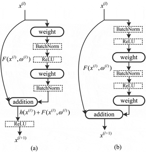
where x^(l) is the input of the l-th building block, F is the residual function, ω^(l) is a set of weights related to the l-th building block. The residual function F(x^(l), ω^(l)) is to be learned. In Figure 1(a), the residual block contains two layers, thus passing over two layers in the skip connection. The operation h + F is performed by a skip connection and element-wise addition. After the addition, the second nonlinearity f is used. f represents the activation function, which adopts a rectified linear unit (ReLU) (Nair and Hinton 2010) in our study. ReLU, which is expressed as f(x) = max(0, x), is able to accelerate the convergence of deep CNNs compared to the tanh (f(x) = tanh(0, x)) or sigmoid (f(x) = (1 + e^−x)⁻¹) function (Krizhevsky, Sutskever, and Hinton 2012). The first version of ResNet consists of the above introduced residual blocks.

In the improved residual unit (Figure 1(b)), h and f are both set as identity mappings, h(x^(l)) = x^(l) and x^(l+1) = y^(l), and thus x^(l+1) can be rewritten as,

(3) $x^{\left(l+1\right)}=x^{(l)}+F(x^{(l)},{\omega }^{\left(l\right)})$(3)

For any deeper block L and any shallower block l, the feature x^(L) can be represented by Equation (4) (He et al. 2016b):

(4) $x^{(L)}={\mathrm{x}}^{(l)}+{\sum }_{i=l}^{L-1}F(x^{\left(i\right)},{\omega }^{\left(i\right)})$(4)

Equation (4) shows that the features x^(L) and x^(l) are modeled in a residual way. Moreover, backward propagation properties can be explored from Equation (4). Suppose J is the loss function, we have:

(5) $\frac{\mathrm{\partial }J}{\mathrm{\partial }{x}^{(l)}}=\frac{\mathrm{\partial }J}{\mathrm{\partial }{x}^{(L)}}\left(1+\frac{\mathrm{\partial }}{\mathrm{\partial }{x}^{(l)}}{\sum }_{i=l}^{L-1}F\left(x^{\left(i\right)},{\omega }^{\left(i\right)}\right)\right)$(5)

Equations (4) and (5) show that features at different levels can be directly propagated, both forward and backward. Additionally, the new residual unit (Figure 1(b)) uses BatchNorm and ReLU before weight layers, which simplifies the training process of deeper networks, and improves the accuracy (He et al. 2016b).

From the above introduction of residual units, we note that convolutional layers are in the ResNet. Given an input volume of size W × H × C in layer L, where W is the width of the feature map, H is the height of the feature map and C is the number of feature maps. Each unit in the W × H feature map is connected to a local region of size f × f × n in the feature maps of layer L − 1, where f is the kernel size and n is the number of filters. In other words, each unit in the W × H feature map is the position of a local feature.

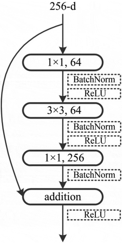
ResNet-101 is a ResNet-based network. Its building block contains a stack of three layers. A building block of the first group of residual units of ResNet-101 is shown in Figure 2. The first 1 × 1 layer is used to reduce dimension while the last one is to restore dimension. Using the modified residual unit (Figure 1(b)) instead of the original one (Figure 1(a)), ResNet-101-v2 is presented. In this paper, we use the convolutional layers of ResNet-101-v2 to learn high-level features.

Figure 2. A building block with a bottleneck design for ResNet-101 (He et al. 2016a).

3.2. Global representation using deep features

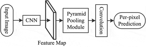
Features learned by deep FCNs (Long, Shelhamer, and Darrell 2015) are lack of effective global information. To include global features for complex scene parsing, Zhao et al. (2017a) proposed the PSPNet. The general architecture of PSPNet is illustrated in Figure 3. Given an input image, it uses a deep CNN to extract the convolutional feature map. On top of it, a pyramid pooling module is applied to gather features from different sub-regions. The multi-level features are upsampled and concatenated with the original CNN features to form the representation map, which is followed by a convolutional layer to predict pixel-level labels. The feature representation used in PSPNet contains both local and global contexts.

Figure 3. Overview of the PSPNet (Zhao et al. 2017a).

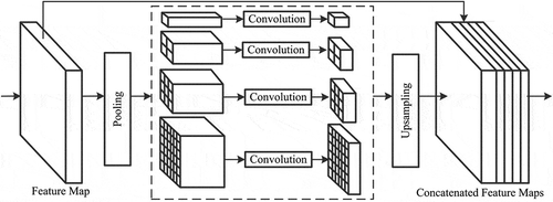
PSPNet extracts effective global contexts for scene parsing. The pyramid pooling module is capable of collecting multi-level global information. Its structure is illustrated in Figure 4. Given the last layer of the convolutional feature map, multiple pyramid scales are applied to generate multi-scale features. The coarsest level generates a single output (shown in the first row inside the dashed line box of Figure 4) while the rest pyramid levels all contain context features based on sub-regions. Each pyramid level is followed by a 1 × 1 convolution layer to reduce the feature dimension to the reciprocal of the pyramid level size, thus maintaining the weight of the global feature. The low-dimension feature maps are then upsampled to get the same size as the input feature map by bilinear interpolation. Finally, these multi-scale features are fused as the global feature. The pyramid pooling module effectively reduces context information loss among multiple sub-regions, which aids various categories detection.

Figure 4. Pyramid pooling module (Zhao et al. 2017a).

3.3. The proposed deep learning architecture

With ResNet-101-v2 (He et al. 2016b) and the pyramid pooling module (Zhao et al. 2017a) introduced above, our proposed deep learning architecture is illustrated in Figure 5. Given a high resolution remote sensing image, we use the ResNet-101-v2 model to learn deep CNN features. The first convolutional layer of ResNet-101-v2 applies 64 filters with the size of 7 × 7 at stride 2 to the input image. Four groups of 3-layer blocks with a bottleneck design are then performed. For example, in the first building block, the first convolutional layer applies 64 filters with the size of 1 × 1, the second convolutional layer applies 64 filters with the size of 3 × 3, and the third convolutional layer applies 256 filters with the size of 1 × 1. See Figure 5 for detailed architecture. On top of the last convolutional layer in ResNet-101-v2, pyramid pooling module is applied to collect multi-level global information from high resolution remote sensing images. Specifically, a four-level pyramid pooling module is adopted, with bin sizes of 1 × 1, 2 × 2, 3 × 3 and 6 × 6. Low-dimension context representations are then upsampled by bilinear interpolation, thus obtaining representations with the same size as the original feature map. Finally, we concatenate multi-level global features and the last-layer convolutional feature map for the pixel-wise prediction.

Figure 5. Overview of our proposed deep neural network.

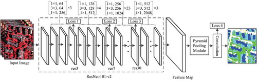
The original PSPNet (Zhao et al. 2017a) adds one auxiliary loss in the training phase. This strategy helps optimize the learning process and shows generality in their experiments. Taking this learning strategy into consideration, we propose adding multiple additional losses to our end-to-end network. In detail, we generate results for each group of building blocks by supervision with an additional loss. As shown in Figure 5, Losses 1–3 are added after the third, seventh and thirtieth residual units according to the architecture of the ResNet-101-v2 model. Loss 4 after the last convolutional layer in the main branch is to train the final classifier. In this way, the optimization of the proposed deep network is divided into several parts according to the number of auxiliary losses. Each part is easier to solve than the original network. As the loss in the main branch takes the major responsibility (Zhao et al. 2017a), we add weights to each auxiliary loss to balance these losses. In this paper, the auxiliary losses used are all softmax loss function (Equations (6) and (7)),

(6) $loss=-s^{\left(y^{\left(i\right)}\right)}+\mathrm{l}\mathrm{o}\mathrm{g}{\sum }_j{e}^{s^{\left(j\right)}}$(6)

(7) $s=f(x^{\left(i\right)};{\omega }^{\left(i\right)})$(7)

Given an image dataset, y is the label, x is the input image and $\omega$ is the weights.

4. Experiments

4.1. Dataset

To evaluate the performance of the proposed approach, two challenging and standard airborne image datasets, the Vaihingen and Potsdam datasets, are used in the experiments. These two datasets are from 2D Semantic Labeling Contest held by the International Society for Photogrammetry and Remote Sensing (ISPRS).¹ There are six ground object categories in the datasets, comprising impervious surfaces, building, low vegetation, tree, car and clutter/background. The clutter/background category includes ground objects like water bodies, containers, tennis courts and swimming pools.

Vaihingen is a small village in Germany. The Vaihingen dataset consists of 33 image patches, and each patch comprises true orthophoto (TOP) tiles and digital surface models (DSMs) with a spatial resolution of 9 cm. There are 3 bands in the TOP tiles, including near-infrared, red and green channels. Particularly, 16 out of 33 tiles involve labeled ground truth. These 16 TOP tiles are used to train the semantic segmentation model while the other 17 TOP tiles are used for testing. The dimensions of the tiles in the Vaihingen dataset are shown in Table 1. The Potsdam dataset contains 38 patches with 6000 × 6000 pixels each, which comprises TOP and DSM files. Each TOP file consists of red, green, blue and infrared bands. The spatial resolution of TOP and DSM is 5 cm. And 24 out of 38 patches are provided with ground truth and only the 24 TOP files with red, green and infrared bands are used for training the segmentation model. The rest 14 TOP patches are used to evaluate the model by the ISPRS organization.

Table 1. The dimensions of 16 TOP tiles in the training set and 17 TOP tiles in the testing set.

Tiles in the training set			Tiles in the testing set
Patch Number	Column	Row	Patch Number	Column	Row
1	1919	2569	2	2428	2767
3	2006	3007	4	1887	2557
5	1887	2557	6	1887	2557
7	1887	2557	8	1887	2557
11	1893	2566	10	1887	2557
13	2818	2558	12	1922	2575
15	1919	2565	14	1919	2565
17	2336	1281	16	1919	2565
21	1903	2546	20	1866	2315
23	1903	2546	22	1903	2546
26	2995	1783	24	1903	2546
28	1917	2567	27	1917	3313
30	1934	2563	29	1917	2563
32	1980	2555	31	1980	2555
34	1388	2555	33	1581	2555
37	1996	1995	35	2805	1884
			38	3816	2550

4.2. Evaluation metrics

The evaluation strategy from 2D Semantic Labeling Contest relies on the pixel-based confusion matrix. Two evaluation strategies are employed. The first is a standard evaluation with full references in the test images. The second evaluation ignores the eroding edges with a 3-pixel circular disc in the ground truth. Recall (R), precision (P), F1 score and overall accuracy (OA) are computed based on the confusion matrix. R demonstrates the ratio of correctly predicted pixels with regard to the total number of pixels in that ground truth class.

(8) $R=\frac{TP}{TP+FN}$(8)

where TP is the number of true positive pixels and FN is the false negative pixels.

P shows the proportion of correctly predicted pixels with regard to the total number of pixels classified as this class in the final prediction.

(9) $P=\frac{TP}{TP+FP}$(9)

where FP is the number of false positive pixels.

F1 score is defined by the following equation:

(10) $\mathrm{F}1=2\frac{P\times R}{P+R}$(10)

in which P and R are weighted equally. The last measure, OA, represents the ratio of correctly classified test samples globally.

4.3. Details of implementation

We use a pre-trained ResNet-101-v2 model trained on the ImageNet dataset² to partially initialize the network. Then we finetune the model on the whole training set of aerial images. Considering the limitation of the hardware, the dense labeled TOP tiles of Vaihingen and Potsdam datasets are divided into patches with 500 × 500 pixels. There is a 200-pixels overlap between neighboring images. In order to resist overfitting, several strategies are adopted. We perform random mirror to augment training data by flipping the image from left to right. The input images are rescaled by 0.5, 0.75, 1.0, 1.25, 1.5, which accords with the strategy of PSPNet (Zhao et al. 2017a). Random crop is another strategy used by Zhao et al. (2017a) in data augmentation, which has been proved effective. We randomly crop the image to 393 × 393 pixels from the patches.

Our experiments are carried out on the Caffe deep learning framework (Jia et al. 2014). Inspired by the works in (Zhao et al. 2017a; Chen et al. 2018b), a “poly” learning rate policy is employed, which calculates the current learning rate by the product of the base rate using (1-iter/max_iter)^power. The base learning rate and power are set to 0.0001 and 0.9 respectively. Following the implementation details in Zhao et al. (2017a), we use momentum of 0.9 and weight decay of 0.0001. The maximum iteration number is 200K. In addition, the auxiliary losses are weighted by 0.4. All the experiments are conducted on a machine equipped with two Nvidia Titan X GPUs with Pascal architecture and 12 GB frame buffer. Due to the memory limit of GPUs, the batch size is fixed to 1. The training phase took about 3 days and the testing phase took about 2 hours in the experiments.

5. Results and discussion

5.1. Vaihingen data

Deep models show good performance in semantic segmentation tasks (Zhao et al. 2017a; Badrinarayanan, Kendall, and Cipolla 2017). However, simply stacking more layers does not guarantee better performance. As the depth gets deeper, accuracy becomes saturated by the degradation problem (He et al. 2016a). A residual learning framework, with skip connection in the building block, is proposed to address this problem (He et al. 2016b, 2016a). Features at deeper blocks can be computed by adding features at shallower blocks to the preceding residues. Apart from the residual units used in the network, we further propose a strategy for the optimization of the ResNet-101-v2 model. We use the supervised method to generate initial results on multi-resolution images with additional losses and compute the residue with the final loss. Different from the architecture in Zhao et al. (2017a), at least two auxiliary losses are added to optimize the training process. To illustrate the effectiveness of the auxiliary losses, experiments with a different number of auxiliary losses are conducted. Using the whole ground truth dataset, the testing results are shown in Table 2. All the experiments are with the master branch’s softmax loss (Loss 4 shown in Figure 5). PSPNet, considered as the baseline, adds Loss 3 (Figure 5) in the network. The networks with at least two auxiliary losses outperform the baseline with an improvement of 0.90–1.00 in terms of OA (%). The network with Loss 2 and 3 and that with Loss 1, 2 and 3 produce similar results in the Vaihingen data. We further conduct Cochran’s Q test (Cochran 1950) on the testing results in Table 2. The classification results of Vaihingen data are significantly different at the 0.05 level. This indicates the effectiveness of the supervised training strategy with two or more auxiliary losses.

Table 2. Experimental results with a different number of auxiliary losses. Loss 1, 2 and 3 are shown in Figure 5.

Method	OA(%)
	Vaihingen dataset	Potsdam dataset
ResNet101-v2(with Loss 3)	84.70	71.90
ResNet101-v2(with Loss 2 and 3)	85.70	87.80
ResNet101-v2(with Loss 1, 2 and 3)	85.60	88.00

To further evaluate the quantitative results, the semantic segmentation results are compared with that of three approaches, superpixel-based classification using the stair vision library (SP-SVL-3) (Gerke 2014), a structured Haar wavelet-based convolutional neural network (CNN-HAW) (Tschannen et al. 2016) and CNN-based full patch labeling by learned upsampling (CNN-FPL) (Volpi and Tuia 2017). These approaches are selected from the ISPRS leaderboard³ because they consider all the six ground object categories in the detection results. SP-SVL-3 is a traditional object-based method. It classifies the Vaihingen images using hand-crafted features including SVL-features, NDVI, saturation and normalized height. CNN-HAW and CNN-FPL are both pixel-based methods. CNN-HAW uses multi-scale features extracted by a tree-like CNN (Tschannen et al. 2016). CNN-FPL adopts CNN features synthesizing contextual relationships by a downsample-then-upsample architecture.

Using the whole ground truth dataset, the evaluation results of the Vaihingen test images are presented (Table 3). From Table 3, we can recognize that the proposed method outperforms all the other methods with an OA of 85.7%. Additionally, we can observe that the OAs of the methods using deep features outperform that of SP-SVL-3 using the hand-crafted features. Concerning the performance of each class, R, P and F1 score of our methods are higher than that of SP-SVL-3, CNN-HAW, and CNN-FPL. The results evaluated by the references with eroded boundaries are listed in Table 4. Besides SP-SVL-3, CNN-HAW, and CNN-FPL, a two parallel SegNet (SegNet-p) is demonstrated in Table 4. SegNet-p (Marmanis et al. 2018) processes the color images and DSMs in two SegNet branches separately. We can observe that the OA of each approach shown in Table 3 is lower than that presented in Table 4. This indicates that uncertain labels exist on the eroded boundaries with the circle of 3-pixel radius. In addition, our method obtains a 3.9 percentage point increase over SegNet-p. However, the building detection rate of SegNet-p reaches 93.8%, a gain of 0.6 percentage points over our method. We think this is because SegNet-p learns height characteristics through the SegNet with an input of DSM and normalized DSM data.

Table 3. Evaluation of results in the Vaihingen dataset using the full reference set.

Methods		Impervious Surfaces	Buildings	Low Vegetation	Trees	Cars	Clutter
SP-SVL-3 (Gerke 2014)	Precision	81.00	89.90	76.10	79.60	63.20	30.50
	Recall	86.50	88.00	71.00	84.50	42.80	0.70
	F1	83.60	88.90	73.40	82.00	51.00	1.30
	OA	81.80
CNN-HAW (Tschannen et al. 2016)	Precision	84.70	87.90	77.80	80.20	50.00	68.80
	Recall	83.20	91.60	69.90	88.00	52.20	18.30
	F1	83.90	89.70	73.60	83.90	51.10	28.90
	OA	82.60
CNN-FPL (Volpi and Tuia 2017)	Precision	84.30	90.10	77.70	84.50	71.70	53.60
	Recall	88.40	90.80	78.40	83.30	38.70	2.10
	F1	86.30	90.50	78.00	83.90	50.30	4.10
	OA	84.30
Our method	Precision	86.50	90.80	79.50	84.40	83.00	97.20
	Recall	89.60	91.90	77.80	85.90	50.40	18.00
	F1	88.00	91.30	78.60	85.20	62.70	30.30
	OA	85.70

Table 4. OAs of results in the Vaihingen dataset using the reference set with eroded boundaries.

Methods	OA
SP-SVL-3 (Gerke 2014)	84.80
CNN-HAW (Tschannen et al. 2016)	85.90
CNN-FPL (Volpi and Tuia 2017)	87.30
SegNet-p (Marmanis et al. 2018)	84.80
Our method	88.70

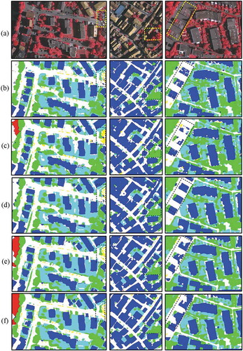
To visualize the evaluation results, we demonstrate three examples in Figure 6. In terms of cars, our method shows an improvement as we consider both local and global deep features. For example, in the dash-line box of the first column in Figure 6, our method is able to predict the car class correctly while the other four approaches mistake cars as buildings. For the background objects, all the methods show poor performance, especially SP-SVL-3 and CNN-FPL. In the top left corner of the first column in Figure 6, only CNN-HAW, PSPNet and our method correctly predict part of water. With respect to low vegetation and trees, our method shows a good performance in a complex situation. As shown in the dash-line box of the second column in Figure 6, trees and low vegetation in shade are mixed together. Our network distinguishes low vegetation in shade from trees while other methods confuse them. For buildings, the results by SP-SVL-3, CNN-HAW and CNN-FPL methods all perform well, because the DSM channel is considered in these methods. For example, in the dash-line box of the third column in Figure 6, height information reduces the confusion between impervious surfaces and buildings. However, due to the spectral similarity, parts of buildings are mistaken as impervious surfaces in the prediction of SP-SVL-3 and CNN-HAW.

Figure 6. Example results of test images in the Vaihingen dataset. (a) The original image, (b) the results of SP-SVL-3, (c) the results of CNN-HAW, (d) the results of CNN-FPL, (e) the results of PSPNet and (f) our results. White: impervious surfaces, Blue: buildings, Cyan: low vegetation, Green: trees, Yellow: cars, Red: clutter/background. (Best viewed in color version).

5.2. Potsdam data

Similar to the Vaihingen data, we submitted our predictions of test tiles in the Potsdam dataset to ISPRS to evaluate the proposed model.⁴ Networks with different auxiliary losses are evaluated (Table 2). Three methods in Table 2 all contain the master branch’s softmax loss (Loss 4 shown in Figure 5). As expected, both the network with Loss 2 and 3 and that with Loss 1, 2 and 3 improve the classification accuracy (Table 2) in the Potsdam data. And Cochran’s Q test indicates significant differences among the three classifications of Potsdam data (Table 2) at the 0.05 level. This is similar to the Vaihingen data. However, the OA gain in the Potsdam dataset is greater than that in the Vaihingen data. In detail, the network with Loss 2 and 3 and that with Loss 1, 2 and 3 outperform the model with Loss 3 (PSPNet) by 15.90 and 16.10 in terms of OA (%), respectively. Because the size of the training set in the Potsdam dataset is larger than that in the Vaihingen dataset. Moreover, scenes in the Potsdam dataset are more complex than that in the Vaihingen dataset.

In addition, we compare our results with that of SP-SVL-3 (Gerke 2014), CNN-FPL (Volpi and Tuia 2017) and deep convolutional neural network (DCNN) (Kemker, Salvaggio, and Kanan 2017). Table 5 demonstrates the accuracies of all the methods using the whole ground truth. Our network achieves the best performance among the four methods with an OA of 88.00%. Specifically, OAs of approaches with CNN features show a substantial improvement compared with that of SP-SVL-3 with hand-designed features. Nevertheless, with the help of the DSM channel, P, and R of buildings using SP-SVL-3 obtain scores higher than 90.00% (Table 5), which is comparable with the other methods. With respect to F1 score of each class, our method is the highest in Table 5. Table 6 presents the evaluation by the ground truth ignored eroded edges. In terms of OAs, we observe that our method shows an increase of 3.7 to 12.6 points in comparison with the other approaches. The results indicate the effectiveness of the combination of local and multi-level global features used in our network.

Table 5. Evaluation of results in the Potsdam dataset using the full reference set.

Methods		Impervious Surfaces	Buildings	Low Vegetation	Trees	Cars	Clutter
SP-SVL-3 (Gerke 2014)	Precision	77.80	90.00	65.10	69.00	79.60	36.70
	Recall	84.90	90.60	75.70	55.00	45.20	19.40
	F1	81.20	90.30	70.00	61.20	57.60	25.40
	OA	75.40
CNN-FPL (Volpi and Tuia 2017)	Precision	85.80	94.60	80.60	72.60	80.40	47.50
	Recall	88.70	93.70	77.60	83.70	82.30	19.60
	F1	87.20	94.10	79.00	77.70	81.30	27.70
	OA	83.40
DCNN(Kemker, Salvaggio, and Kanan 2017)	Precision	85.60	91.30	78.10	84.00	87.00	58.40
	Recall	89.50	91.50	84.70	78.80	84.40	31.00
	F1	87.60	91.40	81.20	81.30	85.70	40.50
	OA	84.40
Our method	Precision	89.00	93.70	82.10	87.40	91.60	74.80
	Recall	92.00	96.30	87.50	82.80	88.60	39.40
	F1	90.50	95.00	84.70	85.00	90.10	51.60
	OA	88.00

Table 6. OAs of results in the Potsdam dataset using the reference set with eroded boundaries.

Methods	OA
SP-SVL-3 (Gerke 2014)	77.80
CNN-FPL (Volpi and Tuia 2017)	85.80
DCNN (Kemker, Salvaggio, and Kanan 2017)	86.70
SegNet-p (Marmanis et al. 2018)	84.90
Our method	90.40

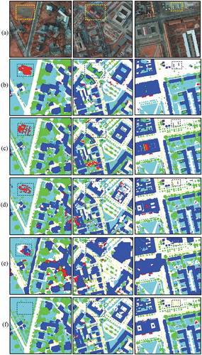
Three examples of evaluation results in the Potsdam dataset are selected (Figure 7). The original images are shown in Row (a) and results by SP-SVL-3 (Gerke 2014), CNN-FPL (Volpi and Tuia 2017), DCNN (Kemker, Salvaggio, and Kanan 2017), PSPNet and our method are displayed in Row (b)–(f), respectively. With respect to the low vegetation and tree classes, our method is able to predict trees surrounded by the low vegetation in the dash-line box of the first column in Figure 7. However, all the other approaches falsely label low vegetation as clutter or buildings. Besides, CNN-FPL correctly predicts trees and SP-SVL-3 and DCNN mistake trees as low vegetation. We think this is because our network not only learns the characteristics of trees and low vegetation themselves but also learns the global contexts of the low vegetation and trees classes. From the perspective of cars, our method shows an improvement compared with the other methods. For instance, in the dash-line box of the third column in Figure 7, our method correctly predicts cars. However, SP-SVL-3 mistakes cars as buildings. CNN-FPL, DCNN, and PSPNet recognize some of the cars as buildings and clutter/background. In terms of buildings, we observe that the predictions of roofs with a complex structure by all the methods are not accurate (in the dash-line box of the second column in Figure 7). The buildings are mistaken as trees or clutter due to the similarities in color or height. We also notice that the clutter class is hard to model in this dataset due to the complicated inner structure and its appearance similar to other classes.

Figure 7. Example results of test images in the Potsdam dataset. (a) the original image, (b) the results of SP-SVL-3, (c) the results of CNN-HAW, (d) the results of CNN-FPL, (e) the results of PSPNet and (f) our results. White: impervious surfaces, Blue: buildings, Cyan: low vegetation, Green: trees, Yellow: cars, Red: clutter/background. (Best viewed in color version).

Although the proposed network shows improvements in the accuracy, there are still some limitations. The input images of the proposed network only contain three bands. This is usually the case in the computer vision field, which deals with color images containing red, green and blue channels. However, high resolution remote sensing images generally contain four bands, i.e. red, green, blue and infrared bands. In our experiments, we only use three bands, infrared, red and green bands, in both the Vaihingen and Potsdam data. Another limitation is that we did not consider the DSMs in both of the datasets. Therefore, the characteristics of images learned by the model are all from the three bands without considering the height information, which is helpful in the classification of buildings/impervious surfaces and trees/low vegetation.

6. Conclusion

In this paper, we propose an end-to-end framework to extract local and global deep features from very high spatial resolution remotely sensed images for semantic segmentation. The deep architecture adopts the advantages of deep residual networks and pyramid pooling network. Auxiliary losses are added to optimize the model by converging to a higher accuracy. We applied the proposed deep network to two public datasets, Vaihingen and Potsdam from ISPRS organization. The results show that models built on deep CNN features perform better than that with hand-crafted features. Our model, synthesizing local and global deep features outperforms that using general CNN features. Moreover, the auxiliary losses added in the network are effective in increasing the model accuracy.

Acknowledgements

The authors would thank the ISPRS provided the Vaihingen and Potsdam datasets.

Disclosure statement

No potential conflict of interest was reported by the authors.

Additional information

Funding

This work was supported by the National Key Research and Development Program of China under Grant number 2017YFB0503600; the National Natural Science Foundation of China under Grant numbers 41601451, 41631179; Zhejiang Provincial Natural Science Foundation of China under Grant number LQ19D010006; the Natural Science Foundation of Beijing, China under Grant number 4172064; the Key Laboratory of Oceanographic Big Data Mining & Application of Zhejiang Province under Grant number OBDMA201512; and the International Partnership Program of the Chinese Academy of Sciences under Grant numbers 131C11KYSB20160061, 131551KYSB20160002.

Notes

1. http://www2.isprs.org/commissions/comm3/wg4/semantic-labeling.html.

2. https://github.com/tornadomeet/ResNet.

3. http://www2.isprs.org/commissions/comm2/wg4/vaihingen-2d-semantic-labeling-contest.html.

4. http://www2.isprs.org/commissions/comm2/wg4/potsdam-2d-semantic-labeling.html.

References

- Arnab, A., S. Jayasumana, S. Zheng, and P. Torr. 2016. “Higher Order Conditional Random Fields in Deep Neural Networks.” In ECCV 2016, 524–540. Amsterdam, The Netherlands: Springer, Cham.
- Audebert, N., B. Le Saux, and L. Sébastien. 2018. “Beyond RGB: Very High Resolution Urban Remote Sensing with Multimodal Deep Networks.” ISPRS Journal of Photogrammetry and Remote Sensing 140: 20–32. doi:10.1016/j.isprsjprs.2017.11.011.
- Badrinarayanan, V., A. Kendall, and R. Cipolla. 2017. “SegNet: A Deep Convolutional Encoder-Decoder Architecture for Image Segmentation.” IEEE Transactions on Pattern Analysis and Machine Intelligence 39 (12): 2481–2495. doi:10.1109/TPAMI.2016.2644615.
- Blaschke, T. 2010. “Object Based Image Analysis for Remote Sensing.” ISPRS Journal of Photogrammetry and Remote Sensing 65 (1): 2–16. doi:10.1016/j.isprsjprs.2009.06.004.
- Chen, G., Q. Weng, G. J. Hay, and Y. He. 2018a. “Geographic Object-Based Image Analysis (GEOBIA): Emerging Trends and Future Opportunities.” GIScience & Remote Sensing 55 (2): 159–182. doi:10.1080/15481603.2018.1426092.
- Chen, L. C., G. Papandreou, I. Kokkinos, K. Murphy, and A. L. Yuille. 2018b. “DeepLab: Semantic Image Segmentation with Deep Convolutional Nets, Atrous Convolution, and Fully Connected CRFs.” IEEE Transactions on Pattern Analysis & Machine Intelligence 40 (4): 834–848. doi:10.1109/TPAMI.2017.2699184.
- Cleve, C., M. Kelly, F. R. Kearns, and M. Moritz. 2008. “Classification of the Wildland–Urban Interface: A Comparison of Pixel-And Object-Based Classifications Using High-Resolution Aerial Photography.” Computers, Environment and Urban Systems 32 (4): 317–326. doi:10.1016/j.compenvurbsys.2007.10.001.
- Cochran, W. G. 1950. “The Comparison of Percentages in Matched Samples.” Biometrika 37 (3/4): 256–266. doi:10.2307/2332378.
- Cordts, M., M. Omran, S. Ramos, T. Rehfeld, M. Enzweiler, R. Benenson, U. Franke, S. Roth, and B. Schiele. 2016. “The Cityscapes Dataset for Semantic Urban Scene Understanding.” In 2016 IEEE Conference on Computer Vision and Pattern Recognition (CVPR), 3213–3223. Las Vegas, NV, USA: IEEE.
- Gerke, M. 2014. “Use of the Stair Vision Library within the ISPRS 2D Semantic Labeling Benchmark (Vaihingen).” doi: 10.13140/2.1.5015.9683.
- Girshick, R., J. Donahue, T. Darrell, and J. Malik. 2014. “Rich Feature Hierarchies for Accurate Object Detection and Semantic Segmentation.” In 2014 IEEE Conference on Computer Vision and Pattern Recognition, 580–587. Columbus, OH, USA: IEEE.
- He, K., X. Zhang, S. Ren, and J. Sun. 2016a. “Deep Residual Learning for Image Recognition.” In 2016 IEEE Conference on Computer Vision and Pattern Recognition (CVPR), 770–778. Las Vegas, NV, USA: IEEE.
- He, K., X. Zhang, S. Ren, and J. Sun. 2016b. “Identity Mappings in Deep Residual Networks.” In European Conference on Computer Vision, 630–645. Amsterdam, The Netherlands: Springer, Cham.
- Jia, Y., E. Shelhamer, J. Donahue, S. Karayev, J. Long, R. B. Girshick, S. Guadarrama, and T. Darrell. 2014. “Caffe: Convolutional Architecture for Fast Feature Embedding.” ACM Multimedia:675–678.
- Jiao, L., M. Liang, H. Chen, S. Yang, H. Liu, and X. Cao. 2017. “Deep Fully Convolutional Network-Based Spatial Distribution Prediction for Hyperspectral Image Classification.” IEEE Transactions on Geoscience and Remote Sensing 55 (10): 5585–5599. doi:10.1109/TGRS.2017.2710079.
- Kemker, R., C. Salvaggio, and C. Kanan. 2017. “Algorithms for Semantic Segmentation of Multispectral Remote Sensing Imagery Using Deep Learning.” ISPRS Journal of Photogrammetry and Remote Sensing 145: 60–77. doi:10.1016/j.isprsjprs.2018.04.014.
- Krizhevsky, A., I. Sutskever, and G. E. Hinton. 2012. “ImageNet Classification with Deep Convolutional Neural Networks.” In Neural Information Processing Systems, 1097–1105. Lake Tahoe, Nevada: Curran Associates Inc., USA.
- LeCun, Y., Y. Bengio, and G. Hinton. 2015. “Deep Learning.” Nature 521 (7553): 436–444. doi:10.1038/nature14539.
- Liu, T., A. Abd-Elrahman, J. Morton, and V. L. Wilhelm. 2018. “Comparing Fully Convolutional Networks, Random Forest, Support Vector Machine, and Patch-Based Deep Convolutional Neural Networks for Object-Based Wetland Mapping Using Images from Small Unmanned Aircraft System.” GIScience & Remote Sensing 55 (2): 243–264. doi:10.1080/15481603.2018.1426091.
- Long, J., E. Shelhamer, and T. Darrell. 2015. “Fully Convolutional Networks for Semantic Segmentation.” In 2015 IEEE Conference on Computer Vision and Pattern Recognition (CVPR), 3431–3440. Boston, MA, USA: IEEE.
- Maggiori, E., Y. Tarabalka, G. Charpiat, and P. Alliez. 2017. “Convolutional Neural Networks for Large-Scale Remote-Sensing Image Classification.” IEEE Transactions on Geoscience and Remote Sensing 55 (2): 645–657. doi:10.1109/TGRS.2016.2612821.
- Marmanis, D., K. Schindler, J. D. Wegner, S. Galliani, M. Datcu, and U. Stilla. 2018. “Classification with an Edge: Improving Semantic Image Segmentation with Boundary Detection.” ISPRS Journal of Photogrammetry and Remote Sensing 135: 158–172. doi:10.1016/j.isprsjprs.2017.11.009.
- Mboga, N., S. Georganos, T. Grippa, M. Lennert, S. Vanhuysse, and E. Wolff. 2018. “Fully Convolutional Networks for the Classification of Aerial VHR Imagery.” In GEOBIA 2018. Montpellier, France.
- Ming, D., J. Li, J. Wang, and M. Zhang. 2015. “Scale Parameter Selection by Spatial Statistics for GeOBIA: Using Mean-Shift Based Multi-Scale Segmentation as an Example.” ISPRS Journal of Photogrammetry and Remote Sensing 106: 28–41. doi:10.1016/j.isprsjprs.2015.04.010.
- Nair, V., and G. E. Hinton. 2010. “Rectified Linear Units Improve Restricted Boltzmann Machines.” In International Conference on International Conference on Machine Learning, 807–814. Haifa, Israel: Omnipress, USA.
- Noh, H., S. Hong, and B. Han. 2015. “Learning Deconvolution Network for Semantic Segmentation.” In IEEE International Conference on Computer Vision, 1520–1528. Santiago, Chile: IEEE. doi:10.1016/j.jnutbio.2015.07.018.
- Paisitkriangkrai, S., J. Sherrah, P. Janney, and A. van Den Hengel. 2016. “Semantic Labeling of Aerial and Satellite Imagery.” IEEE Journal of Selected Topics in Applied Earth Observations and Remote Sensing 9 (7): 2868–2881. doi:10.1109/JSTARS.2016.2582921.
- Razavian, A. S., H. Azizpour, J. Sullivan, and S. Carlsson. 2014. “CNN Features Off-the-Shelf: An Astounding Baseline for Recognition.” In IEEE Conference on Computer Vision and Pattern Recognition Workshops, 512–519. Columbus, OH, USA: IEEE. doi:10.1177/1753193414530193.
- Ren, S., K. He, R. Girshick, and J. Sun. 2017. “Faster R-CNN: Towards Real-Time Object Detection with Region Proposal Networks.” IEEE Transactions on Pattern Analysis and Machine Intelligence 39 (6): 1137–1149. doi:10.1109/TPAMI.2016.2577031.
- Scott, G. J., R. A. Marcum, C. H. Davis, and T. W. Nivin. 2017. “Fusion of Deep Convolutional Neural Networks for Land Cover Classification of High-Resolution Imagery.” IEEE Geoscience and Remote Sensing Letters 14 (9): 1638–1642. doi:10.1109/LGRS.2017.2722988.
- Sharma, A., X. Liu, X. Yang, and D. Shi. 2017. “A Patch-Based Convolutional Neural Network for Remote Sensing Image Classification.” Neural Networks 95: 19–28. doi:10.1016/j.neunet.2017.07.017.
- Sherrah, J. 2016. “Fully Convolutional Networks for Dense Semantic Labelling of High-Resolution Aerial Imagery.” arXiv Preprint arXiv 1606: 02585.
- Szegedy, C., L. Wei, J. Yangqing, P. Sermanet, S. Reed, D. Anguelov, D. Erhan, V. Vanhoucke, and A. Rabinovich. 2015. “Going Deeper with Convolutions.” In 2015 IEEE Conference on Computer Vision and Pattern Recognition (CVPR), 1–9. Boston, MA, USA: IEEE.
- Taubenböck, H., T. Esch, M. Wurm, A. Roth, and S. Dech. 2010. “Object-Based Feature Extraction Using High Spatial Resolution Satellite Data of Urban Areas.” Journal of Spatial Science 55 (1): 117–132. doi:10.1080/14498596.2010.487854.
- Tschannen, M., L. Cavigelli, F. Mentzer, T. Wiatowski, and L. Benini. 2016. “Deep Structured Features for Semantic Segmentation.” In 25th European Signal Processing Conference, 61–65. Kos, Greece: IEEE.
- Volpi, M., and D. Tuia. 2017. “Dense Semantic Labeling of Subdecimeter Resolution Images with Convolutional Neural Networks.” IEEE Transactions on Geoscience and Remote Sensing 55 (2): 881–893. doi:10.1109/TGRS.2016.2616585.
- Yang, J., Y. Q. Zhao, and J. C. W. Chan. 2017. “Learning and Transferring Deep Joint Spectral-Spatial Features for Hyperspectral Classification.” IEEE Transactions on Geoscience and Remote Sensing 55 (8): 4729–4742. doi:10.1109/TGRS.2017.2698503.
- Zeiler, M. D., and R. Fergus. 2014. “Visualizing and Understanding Convolutional Networks.” In ECCV 2014, 818–833. Zurich, Switzerland: Springer, Cham.
- Zhang, C., X. Pan, H. Li, A. Gardiner, I. Sargent, J. Hare, and P. M. Atkinson. 2018. “A Hybrid MLP-CNN Classifier for Very Fine Resolution Remotely Sensed Image Classification.” ISPRS Journal of Photogrammetry and Remote Sensing 140: 133–144. doi:10.1016/j.isprsjprs.2017.07.014.
- Zhao, B., B. Huang, and Y. Zhong. 2017. “Transfer Learning with Fully Pretrained Deep Convolution Networks for Land-Use Classification.” IEEE Geoscience and Remote Sensing Letters 14 (9): 1436–1440. doi:10.1109/LGRS.2017.2691013.
- Zhao, H., J. Shi, Q. Xiaojuan, X. Wang, and J. Jia. 2017a. “Pyramid Scene Parsing Network.” In 2017 IEEE Conference on Computer Vision and Pattern Recognition (CVPR), 6230–6239. Honolulu, HI, USA: IEEE.
- Zhao, W., S. Du, and W. J. Emery. 2017. “Object-Based Convolutional Neural Network for High-Resolution Imagery Classification.” IEEE Journal of Selected Topics in Applied Earth Observations and Remote Sensing 10 (7): 3386–3396. doi:10.1109/JSTARS.2017.2680324.
- Zhao, W., L. Jiao, W. Ma, J. Zhao, J. Zhao, H. Liu, X. Cao, and S. Yang. 2017b. “Superpixel-Based Multiple Local CNN for Panchromatic and Multispectral Image Classification.” IEEE Transactions on Geoscience and Remote Sensing 55 (7): 4141–4156. doi:10.1109/TGRS.2017.2689018.
- Zhao, W., and D. Shihong. 2016. “Learning Multiscale and Deep Representations for Classifying Remotely Sensed Imagery.” ISPRS Journal of Photogrammetry and Remote Sensing 113: 155–165. doi:10.1016/j.isprsjprs.2016.01.004.
- Zhao, W., D. Shihong, Q. Wang, and W. J. Emery. 2017c. “Contextually Guided Very-High-Resolution Imagery Classification with Semantic Segments.” ISPRS Journal of Photogrammetry and Remote Sensing 132: 48–60. doi:10.1016/j.isprsjprs.2017.08.011.