
 ?Mathematical formulae have been encoded as MathML and are displayed in this HTML version using MathJax in order to improve their display. Uncheck the box to turn MathJax off. This feature requires Javascript. Click on a formula to zoom.
Abstract
Land-cover change may affect water and carbon cycles when transitioning from one land-cover category to another (land-cover conversion, LCC) or when the characteristics of the land-cover type are altered without changing its overall category (land-cover modification, LCM). Given the increasing availability of time-series remotely sensed data for earth monitoring, there has been increased recognition of the importance of accounting for both LCC and LCM to study annual land-cover changes. In this study, we integrated 1,513 time-series Landsat images and a change-updating method to identify annual LCC and LCM during 1986–2015 in the coastal area of Zhejiang Province, China. The purpose was to quantify their contributions to land-cover changes and impacts on the amount of vegetation. The results show that LCC and LCM can be successfully distinguished with an overall accuracy of 90.0%. LCM accounted for 22% and 40.5% of the detected land-cover changes in reclaimed and inland areas, respectively, during 1986–2015. In the reclaimed area, LCC occurred mostly in muddy tidal flats, construction land, aquaculture ponds, and freshwater herbaceous land, whereas LCM occurred mostly in freshwater herbaceous land, Spartina alterniflora, and muddy tidal flats. In the inland area, both LCC and LCM were concentrated in forest and dryland. Overall, LCC had a mean magnitude of normalized difference vegetation index (NDVI) change similar to that of LCM. However, LCC had a positive effect and LCM had a negative effect on NDVI change in the reclaimed area. Both LCC and LCM in the inland area had negative impacts on vegetation greenness, but LCC resulted in larger NDVI change magnitude. Impacts of LCC and LCM on vegetation greenness were quantified for each land-cover type. This study provided a methodological framework to take both LCC and LCM into account when analyzing land-cover changes and quantified their effects on coastal ecosystem vegetation.
Introduction
Land-cover changes generally can be grouped into two types: change between classes and change within classes (Lambin, Geist, and Lepers Citation2003; Lu et al. Citation2004; Lu, Li, and Moran Citation2014). The former is a land-cover conversion (LCC) from one category to a completely different category, such as forest to urban center; the latter is a land-cover modification (LCM) within the same category, such as forest disturbance due to selective logging. Generally, land-cover changes across various landscapes refer to dynamic processes that include both conversion and modification of the earth’s surfaces over time (Alaibakhsh et al. Citation2015; Xu et al. Citation2016). Many previous land-cover change studies focused on conversions not modifications (Lambin, Geist, and Lepers Citation2003; Lu, Li, and Moran Citation2014; Gómez, White, and Wulder Citation2016; Chowdhury et al. Citation2017). This is because many change detection studies were based on the comparison of independent land-cover maps produced at different times with the assumption that only one land-cover change occurred in the time interval (Zhu and Woodcock Citation2014). This assumption is not always valid, especially when images from long time intervals are used or for areas where changes are frequent (Li et al. Citation2017). More important, LCM will not be identified in this kind of application. Therefore, much information may be lost in such land-cover change studies (Turner et al. Citation1995; Zhu Citation2017).
With the development of change detection algorithms based on time series of satellite data, the number of variables and parameters used in characterizing land-cover change have increased rapidly (Parmentier Citation2014; Kennedy et al. Citation2015; Zhu Citation2017). The change-updating method is conceptually appealing, operationally efficient, and economically convenient in these frequent and diverse land-cover change regions in recent years. It updates and backdates the changed areas based on reference date conditions (Gómez, White, and Wulder Citation2016; Huang et al. Citation2017). From the standpoint of mapping and monitoring landscape change using time-series remotely sensed data, there are three general categories: seasonal change, gradual change, and abrupt change (Verbesselt et al. Citation2010; Zhu and Woodcock Citation2014). Among these changes, abrupt change has an immediate impact on land-cover process dynamics and is associated with large magnitude and/or change in the direction of vegetation variation. LCC usually relates to the abrupt change that is induced by deforestation, urbanization, and land reclamation. LCM often corresponds to the abrupt change of plant coverage or species composition caused by floods, fire, or insects. LCM is important for the study of vegetation health condition and for carbon modeling, but difficult to derive from the conventional independent land-cover maps comparison (Zhu and Woodcock Citation2014). Previous research of abrupt change focused primarily on the changes within one land-cover type (Kennedy et al. Citation2012; Zscheischler et al. Citation2013; Devries et al. Citation2015; Hermosilla et al. Citation2016; Shimizu et al. Citation2017). Recently, some studies detected LCC based on the results of abrupt change detection using dense time-series Landsat data (Zhu et al. Citation2016; Li et al. Citation2017). In addition, metrics from Landsat time series can provide extra generic feature space, which is particularly useful for land-cover classification within a stable period (Hansen et al. Citation2014; Gómez, White, and Wulder Citation2016). However, the abrupt change without LCC was taken as false land-cover change and neglected for further analysis. This may be reasonable for areas where abrupt change was mainly induced by LCC, such as in a rapidly developed city, but will omit a large quantity of information in the area where LCM occurred, such as forest and wetland ecosystems.
The free and open Landsat data distribution policy started in 2008 has completely revolutionized the way we utilize Landsat data and has stimulated many novel change detection algorithms based on Landsat time series. The Vegetation Change Tracker (VCT) (Huang et al. Citation2010), Breaks For Additive Seasonal and Trend (BFAST) (Verbesselt et al. 2010), Landtrendr (Kennedy, Yang, and Cohen Citation2010), and Continuous Change Detection and Classification (CCDC) (Zhu and Woodcock Citation2014) algorithms were widely used to detect these types of change features. They provide new capabilities and opportunities to obtain full information about earth surface change and reconsider the traditional algorithms and techniques of land-cover change. The use of dense time-series Landsat data for change detection has increased substantially in recent years and provides the possibility of capturing annual land-cover changes (Hansen et al. Citation2014; Zhu Citation2017; Gómez, White, and Wulder Citation2016; Lu, Li, and Moran Citation2014). For example, the BFAST algorithm uses econometric structural change monitoring to estimate the statistical boundary for determining abrupt change. It is not specific to a particular data type or change agent and can be applied to time series without the need to normalize for land-cover types (Verbesselt et al. 2010). Change detection is entirely data dependent without connection to specific events. This characteristic ensures that it can be used to detect abrupt change in different land-cover types and with different change agents. Recently, the BFAST algorithm has been applied to Landsat time series for detecting forest change (Devries et al. Citation2015; Hamunyela, Verbesselt, and Herold Citation2016), wetland change (Li et al. Citation2017), and land-use history (Dutrieux et al. Citation2016).
To meet the increasing demand for new lands for urban expansion, agriculture, industry, and port expansion, large areas of coastal zones have been reclaimed since the 1980s in Zhejiang Province (Wang et al. Citation2014). Reclamation can be achieved with a number of different methods, including enclosure of tidal flats and filling in the wetland/coastal water bodies using civil materials, clay, dirt, etc. The reclaimed land is gradually constructed into harbors, seawalls, industrial complexes, or urban districts. These processes of land-cover change are exerting immense impacts on coastal environments and ecosystems, adding to the alterations made by natural factors in extreme climate events. These land-cover changes, including both conversion and modification, have affected the regional carbon and water cycles of Zhejiang’s coastal area. However, previous studies mainly focused on LCC without taking LCM into account, thus missing important factors in measuring land-cover change and ignoring certain land-cover change types (Shi et al. Citation2002; Peneva-Reed Citation2014; Wang et al. Citation2017; Hu et al. Citation2017). In this research, we use dense time series of Landsat data to detect abrupt change in the coastal area of Zhejiang Province, China. The objective is to identify LCC and LCM and assess their impacts on vegetation greenness variation in the newly reclaimed and inland areas. This research attempts to answer the following three questions: (1) When did the abrupt change occur over a 30-year period in Zhejiang’s coastal area? (2) How well can LCC and LCM be distinguished and their contributions to the detected abrupt change be quantified through a change-updating method? (3) How much did LCC and LCM influence changes in NDVI (normalized difference vegetation index) during the abrupt change?
Materials and methods
Study area
Zhejiang’s coastal region in southeastern China () was selected for this study. The length of the coastline is up to 1,805 km, accounting for 10% of the mainland coastline of China (Li et al. Citation2018). There are six large bays – Hangzhou, Xiangshan, Taizhou, Sanmen, Yueqing, and Wenzhou – with three main beach types: siltation, erosion, and stable. The silting coastal land is constantly advancing toward the sea, mainly on the south banks of Hangzhou Bay, Taizhou Bay, and Aojiang port to the Oujiang River estuary. The siltation beaches account for approximately 54% of the coastline in Zhejiang, and reclamation activities mainly occurred in these regions. The stable beaches are distributed mainly in the semi-closed harbors, such as Xiangshan Bay and Yueqing Bay. The erosion beaches are distributed mainly in the north of Hangzhou Bay.
Figure 1. Location of the study area in Zhejiang Province, China. (a) The red line is the outer boundary of the study area. The yellow line is the 1984 coastline defined by visual interpretation of the 1984 Landsat imagery. (b) The regions on the land side and on the bay side of the 1984 coastline are defined as inland area and reclaimed area, respectively. Sites 1, 2, and 3 are wetland, dryland, and forest -dominated ecosystems for characterizing typical land-cover and vegetation greenness change processes. (The color composites using the shortwave infrared, near-infrared, and red spectral bands are from the 2016 Landsat 8 Operational Land Imager images (Path118/Rows 39/40/41)).
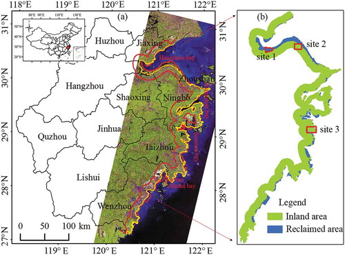
The outer boundary of the study area was manually interpreted based on the 2016 Landsat Operational Land Imager (OLI) images to include the current coastal wetlands such as shallow sea, mud flat, Scirpus mariqueter (hereafter Scirpus), and Spartina alterniflora (hereafter Spartina) and an inward 15-km strip of land along the coastline in 1984 (). The regions on the land side and on the bay side of the 1984 coastline were defined as inland area and reclaimed area, respectively (). These two parts together were called the coastal area of Zhejiang Province. The inland area included some coastal wetland because the 1984 coastline was quantified based on Landsat data in 1984. To compare the difference between LCC and LCM in the reclaimed and inland areas, the statistics were carried out separately for two areas.
Zhejiang’s coastal area has a long land-use history, resulting in complicated land-cover patterns. In the past 30 years, approximately 400,000 ha of tidelands were reclaimed, equivalent to 4.1% of the total area of Zhejiang Province. Starting in 1975, one of the largest single land reclamation projects in Zhejiang Province has been the Xuanmen Land Reclamation Project in Taizhou, Yuhuan County. It has three phases, of which phase II covered 5,330 ha (February 1999 to April 2001), and phase III included 4,530 ha (March 2006 to 2010). Total land reclamation in the Taizhou area between 2004 and 2010, including the project mentioned above, amounted to 26,670 ha. Different land-cover types were formed because of different types of coastal zones and development history. In Hangzhou Bay, farming, including grain and vegetables, is the dominant industry. In Ningbo coastal area, the land-cover is mainly characterized by ports, aquaculture, salt mining, and forestry. The land-cover of Wenzhou coastal area is aquaculture, crops, and forestry. Three typical sites located in Zhejiang’s coastal area were chosen to illustrate the general land-cover and vegetation greenness changes (). Site 1 is a wetland ecosystem reclaimed in the past 30 years located in Hangzhou Bay. Site 2 is a dryland ecosystem including a rapidly developed town in Hangzhou Bay. Site 3 is a forest ecosystem in Ningbo’s coastal area that was disturbed by a large fire in 2004.
Data preparation
Collection of Landsat imagery and calculation of vegetation index
Landsat Thematic Mapper (TM), Enhanced Thematic Mapper Plus (ETM+), and OLI images (Worldwide Reference System Path 118 and Rows 39/40/41) with cloud coverage of less than 80% for the years 1984 to 2016 were downloaded through bulk ordering (https://espa.cr.usgs.gov). A total of 1,513 scenes from Landsat Surface Reflectance Level-2 Science Products (Path 118/Row 39: 431 images; Path 118/Row 40: 480 images; Path 118/Row 41: 602 images) covering Zhejiang’s coastal area were collected (). For Landsat 4-5 TM or Landsat 7 ETM+ data, surface reflectance data were generated from the Landsat Ecosystem Disturbance Adaptive Processing System, a specialized software originally developed through a National Aeronautics and Space Administration (NASA) Making Earth System Data Records for Use in Research Environments grant by NASA Goddard Space Flight Center and the University of Maryland (Masek and Collatz Citation2006). Landsat 8 Surface Reflectance data were generated from the Landsat Surface Reflectance Code, which uses the coastal aerosol band to perform aerosol inversion tests, auxiliary climate data from MODIS, and a unique radiative transfer model. Specific details about the surface reflectance data products can be found in the corresponding product guide. Therefore, the Landsat time-series data can be used directly for calculating vegetation index. The NDVI was calculated due to its easy interpretation and robustness (Jackson and Huete Citation1991), and insensitivity to observation frequency in the time-series analysis (Schultz et al. Citation2016). To ensure that we had enough observations for establishing a time-series model, the pixels with a percentage of NDVI values (not contaminated by cloud, shadow, strip, etc.) less than 20% were deleted in the change detection procedure.
Table 1. The number of Landsat scenes between 1984 and 2016 used in this research.
Collection of land-cover reference data
Based on China’s wetland classification standard, field investigation, and Zhejiang’s actual provincial land-use pattern, a classification scheme with 14 categories was designed for the coastal area (). Field surveys were conducted in 2015 and 2016. The Gaofen-1 satellite imageries with a spatial resolution of 2 m × 2 m, which were acquired in 2015 were used to collect more land-cover sample plots through visual interpretation. Gaofen-1 is a Chinese satellite that was launched on 04/26/2013. This satellite imagery has four multispectral bands (blue, green, red, and near-infrared) with spatial resolutions of 8 m and 16 m, and one panchromatic band with 2 m spatial resolution. A total of 3,400 land-cover reference samples were selected (463 sample plots from field surveys, the rest from Gaofen-1 satellite interpretation), covering different land-covers as shown in .
Table 2. Description of the designed land-cover classification system in this research.
Detection of abrupt change using BFAST
The BFAST algorithm (Verbesselt et al. 2010; Dutrieux et al. Citation2016) was used to detect abrupt change based on NDVI time-series data. This algorithm is a statistical boundary method rooted in econometrics for monitoring structural change (Zeileis et al. Citation2003) and was originally developed for detecting vegetation change in the 16-day Moderate Resolution Imaging Spectroradiometer (MODIS) composite time series (Verbesselt et al. 2010). BFAST can detect multiple breakpoints in time-series regression models using structure change detection (Bai and Perron Citation1998). The method uses a triangular residual sum of squares (RSS) matrix to test the hypothesis that the regression coefficients remain constant over time against the alternative hypothesis that at least one of the coefficients changes in the given regression model (Equation (1)).
where the dependent variable at a given time t (Julian date incorporating year) is expressed as the sum of an overall value β, a sum of different frequency harmonic components representing seasonality and phase (because the sine and cosine functions were combined) a and b, and the slope of a potentially temporal trend in the NDVI time-series data c, the date for the intercept β is a period starts at the time of abrupt change occurred, and T is 365 days per year.
The optimal number of partitions and the position of the breakpoints are determined by minimizing the Bayesian information criterion among all possible partitioning schemes given by the RSS matrix (Bai and Perron Citation2003; Zeileis et al. Citation2003). The unpartitioned time-series regression (Equation (1)) can therefore be re-written for each potential partitioning with Equation (2).
where i is the ith segment, and is the kth breakpoint.
The model coefficients in Equation (2) were estimated by the ordinary least squares method based on the NDVI of each segment. The minimum segment size relative to the sample size was set to 0.10, and the maximum times land-cover change occurred in the study area was set to six (Bai and Perron Citation1998; Dutrieux et al. Citation2016; Li et al. Citation2017). The statistics of detected abrupt changes were started in 1986 and ended in 2015 because the minimum segment size determined a minimum number of clear observations through the moving window. The abrupt change detection was performed using R statistical software with the packages “raster,” “bfast,” “bfastSpatial,” and “strucchange.”
Determination of land-cover conversion and modification
For each abrupt change, land-cover experiences either conversion or modification of the land surface. If the land-cover categories before and after the breakpoint are known, the LCC or LCM occurring at each breakpoint can be identified. Therefore, the first step is to classify the land-cover categories for each segment before and after the abrupt change. We used time-series model coefficients (β, a, b, and c from Equation 2) that characterize seasonal, trend, and overall conditions of vegetation for land-cover classification. These metrics have been proved efficient in land-cover classification (D. Li et al. Citation2017). Based on the change detection, each segment has its parameter set. The mean, median, and standard deviation values of NDVI for each segment were also calculated. Thus, by combining four time-series model parameters (β, a, b, and c), seven variables were used as the input for classification. The random forest classifier was used to perform land-cover classification because of its relatively high accuracy and computational efficiency (Breiman Citation2001; Zhu and Woodcock Citation2014). The 3,400 land-cover reference data were used for training the random forest classifier, and k-fold cross-validation was used for the model evaluation.
Land-cover classification for each stable segment was evaluated to identify and remediate illogical land-cover conversions using temporal filters (Franklin et al. Citation2015 Shih et al. Citation2017). We established temporal conversion filtering to remove illogical class conversions in the context of the study area () based on the field survey and knowledge from local experts and managers. These illogical conversions were taken as the wrong classification and needed further processing. Based on the filter rules in , each LCC was automatically checked for rationality through R. The pixels with illogical conversions were labeled and further interpreted manually based on TimeSync in R and color composites. According to our check results, less than 1% of the pixels were labeled, indicating the robustness of our land-cover change detection method.
Table 3. Acceptable (✓) and illogical (✘) class transitions used in the conversion-rule filter.
Impact of abrupt change on vegetation greenness
For each pixel, the time-series model of each segment was estimated, and the start and end times of each model were also recorded. Equation (3) defined the overall NDVI value for each pixel at the start and end of each segment, and Equation (4) defined the impact of abrupt change on vegetation greenness.
and
where tstart,i and tend,i represent start and end (Julian dates) of the ith segment, and NDVIstart,i and NDVIend,i represent overall NDVI values at the start and end of the ith segment.
Based on the red/near-infrared spectral regions, NDVI is an indicator of chlorophyll abundance and is correlated to vegetation amount and photosynthetic capacity. Positive and negative changes of NDVI over time were referred to as greenness and brownness of vegetation, respectively (Jong et al. Citation2012). Using the land-cover change information for each pixel at the breakpoint, abrupt NDVI change was summarized based on land-cover types, LCC, and LCM. The statistics were based on the prior-date classes to account for the effects of land-cover changes on the greenness in different land-cover types.
Accuracy assessment and validation
A stratified random sample design was used for assessing the change detection accuracy. A total of 1,200 changed/unchanged sample plots can be properly interpreted with the help the TimeSync and high resolution satellite images including Google Earth images and Tiandi maps with high interpretation confidence were selected, of which 600 were from unchanged areas and 600 were selected from changed areas. For the changed samples, 300 were from LCC areas and 300 were from LCM areas. For each sample, the expert manually interpreted the time-series Landsat data, assisted by high spatial resolution imagery, to determine whether the land-cover changed or not (Cohen, Yang, and Kennedy Citation2010). The criterions for correct detection were: the BFAST-detected changes of these sample plots from changed areas occurred in the same year as those manually interpreted, no changes were detected or interpreted in these unchanged plots. The accuracy of distinguishing between LCC and LCM in the samples with land-cover changes was assessed through visual interpretation of temporal Landsat and Google Earth images.
The land-cover reference data previously introduced for land-cover classification were used as the basis for assessing the accuracy of classification. The k-fold cross-validation method was used for the model training and test with the k value set at 10. In k-fold cross-validation, the original 3400 land-cover reference samples are randomly partitioned into k equally sized subsamples. Of the k subsamples, a single subsample is retained as the validation data for testing the model, and the remaining k −1 subsamples are used as training data. The cross-validation process is then repeated k times, with each of the k subsamples used only once as the validation data. The user’s accuracy, producer’s accuracy, and overall accuracy were used to assess the detected changes and land-cover classification results.
Results
Characterizing typical land-cover and NDVI change processes
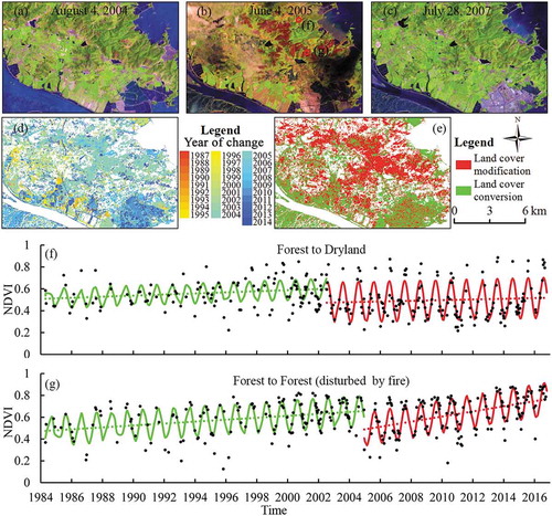
shows the major abrupt change in a reclaimed area and examples of LCC and LCM in muddy tidal flats, including from Spartina to muddy tidal flat and from muddy tidal flat to herbaceous land and an aquaculture pond. These change processes were common in reclaimed areas. The shallow sea was often missed at the beginning of the study period due to insufficient data and little change history at that point. Some transient land-cover types were ignored in the long-term time series. shows the modification in herbaceous land, and the overall and seasonal NDVI show considerable difference among the three segments. This kind of LCM was often induced by the invasion of new species in the herbaceous ecosystem as the reclamation advanced each year. shows a dryland-dominated area with a large proportion of LCC from dryland to construction land. illustrates a very abrupt change in the NDVI value recorded in 2000 from this land-cover change. Construction land also shows seasonality because such pixels were often mixed with plants. shows a modification of dryland that occurred in 2005; the change magnitude was smaller than that of LCC in , and the seasonality was considerably changed after the modification. shows a forest-dominated area experiencing LCM and LCC. shows the land-cover conversion from forest to dryland that occurred in 2002. The mean NDVI indicated a decrease, and the seasonality dynamic increased. shows a modification (forest fire) recorded in 2004 with an abrupt decrease in the NDVI value, and gradual recovery after the disturbance. The seasonality is similar between the two segments. From these examples of different land-cover change processes, the temporal domain information of different land-cover types can be clearly depicted through the dense Landsat NDVI time series, providing a critical foundation for distinguishing LCM and LCC.
Figure 2. Examples of land-cover changes in the wetland ecosystem of Site 1 shown in . (a)–(d) show the color composites (shortwave infrared, near-infrared, and red spectral bands) from Landsat in typical years. (e)–(i) show the times of changes, years in which the latest and penultimate changes occurred, and LCC and LCM. (j)–(m) are the observed NDVI and fitted NDVI using a time-series model for general LCC and LCM in the reclaimed area based on 3 × 3 pixels. Locations of (j)–(m) are shown in (d).
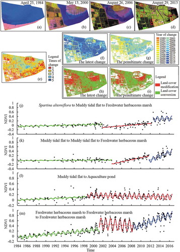
Figure 3. Examples of land-cover changes in the dryland ecosystem of Site 2 shown in . (a)–(c) show the color composites (shortwave infrared, near-infrared, and red spectral bands) from Landsat in typical years. (d) and (e) show the years in which the latest changes occurred, and LCC and LCM. (f) and (g) are the observed NDVI and fitted NDVI using a time-series model for general LCC and LCM in the dryland ecosystem based on 3 × 3 pixels. Locations of (f) and (g) are shown in (c).
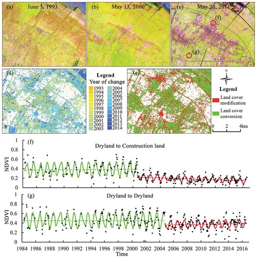
Figure 4. Examples of land-cover changes in the forest ecosystem of Site 3 shown in . (a)–(c) show the color composites (shortwave infrared, near-infrared, and red spectral bands) from Landsat in typical years. (d) and (e) show the years in which the latest changes occurred, and LCC and LCM. (f) and (g) are the observed NDVI and fitted NDVI using a time-series model for general LCC and LCM in the forest ecosystem based on 3 × 3 pixels. Locations of (f) and (g) are shown in (b).
shows the mean values of time-series model coefficients (β, a, b, and c) for each land-cover category based on land-cover reference data. Forest, dryland, and paddy field show higher overall values (β), while herbaceous land, Scirpus, Spartina, muddy tidal flat, and shallow sea are almost equal to 0. Rocky shore and sandy beach showed relatively high overall values. This is mainly because in many places of Zhejiang’s coastal area, the rocky shore and sandy beach are narrow (less than 30 m) and induced many mixed pixels with vegetation. This phenomenon also exists in water pixels because the well-developed but relatively narrow rivers have aquatic and shore vegetation. The trend values (c) indicate that herbaceous land, forest, Scirpus, and Spartina had a considerable tendency toward greenness change, while other land-cover categories showed weak or negligible NDVI change trends. The sea, muddy tidal flats, and mangroves did not show obvious seasonal change, and water and construction land had slight seasonal change due to the mixed pixels containing vegetation and sun angle differences. Dryland, herbaceous land, paddy field, and forest showed the most obvious seasonalities. The different characteristics of coefficients among these land-covers imply that the information contained in the NDVI time-series model is helpful for land-cover classification.
Table 4. The values of four parameters (β intercept, c trend, a harmonic cos, b harmonic sin) in the time-series model based on the 3400 land-cover reference samples and areas for different land-cover classes.
Spatial and temporal characteristics of abrupt change
The change detection accuracy assessment shows that the abrupt change can be retrieved successfully with the overall accuracy of 89.6% (). LCC and LCM can be successfully determined through classifying the divided segments before and after the breakpoint with the overall accuracy of 90.0% (). Land-cover classification yielded an overall accuracy of 86.3% (). The large commission errors occurred among Spartina, herbaceous land, aquaculture ponds, and water, while the large omission errors existed among muddy tidal flats and aquaculture ponds. Overall, abrupt change detection and land-cover classification have confident accuracies for further analysis.
Table 5. Accuracy assessments of abrupt change detection and distinguishing between land-cover conversion and modification based on changed/unchanged samples in China’s Zhejiang Province coastal area.
Table 6. Accuracy of land-cover classification in China’s Zhejiang Province coastal area based on 3400 land-cover reference sample plots collected in 2015–2016.
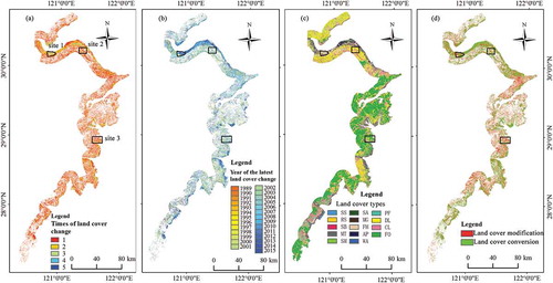
The area statistics of different change times between 1986 and 2015 () indicated that approximately half (49.4%) of Zhejiang’s coastal area has experienced at least one abrupt change in the past 30 years. The once- and twice-changed areas respectively accounted for 69.4% and 24.2% of the total changed area. The abrupt change in the reclaimed area was more widespread with an areal proportion of 84.6%. The proportion of the inland area with abrupt change was lower at 44.5%. The reclaimed area with two abrupt-change breakpoints had the largest proportion, followed by areas with one breakpoint. For the inland area, 77.2% of the total changed area had one breakpoint. Clear boundaries can be seen between reclaimed and inland areas based on number of changes and time of the latest abrupt change (). The highly frequent abrupt changes were located mostly in the estuaries of the rivers emptying to the sea, such as Hangzhou, Sanmen, Taizhou, and Yueqing Bays. For the reclaimed area, the latest abrupt changes occurred mostly after 2007 and concentrated in 2013; for the inland area, the abrupt changes occurred more evenly, mostly during 2001–2013.
Table 7. Area and proportion of change times in China’s Zhejiang Province coastal area between 1986 and 2015.
Figure 5. Numbers of breakpoints (a), the latest change times (b), land-cover types of the latest segments (c), and land-cover conversions and modifications of the latest changes (d) in China’s Zhejiang Province coastal area.
Land-cover conversion and modification
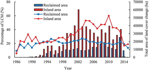
LCM accounted for 35.4% of the abrupt change in Zhejiang’s coastal area during 1986–2015 (). LCM in the reclaimed and inland areas accounted for 22.0% and 40.5% of the total land-cover changes, respectively. The temporal change trends of annual LCM percentage and total change area also varied during 1986–2015 (). In the reclaimed area, less than 30% (ranging from 9% to 27%) of abrupt change was related to LCC in each year. The proportion of breakpoints caused by LCM showed an upward trend during 1985–2003, but a decreased trend between 2004 and 2015. For the inland area, the proportion of LCM showed a considerable increase trend from 1986 to 2005, a high level of stability in 2006–2010, and a sharp downward trend from 2010 to 2014. The LCM amounted to over 50% of abrupt change in 2004, 2005, and 2010. LCC occurred mostly near cities, towns, roads, and reclaimed areas, while LCM was located mostly in forest and dryland of the inland area and protected wetland regions in the reclaimed area ().
Table 8. Summary of land-cover conversion and modification in China’s Zhejiang Province coastal area.
Figure 6. Percentage of land-cover modification (line) to abrupt change and total area of abrupt change (histogram) in the reclaimed and inland areas of China’s Zhejiang Province coast during 1986–2015.
LCC and LCM strongly related to different land-cover types in the coastal area (). In the reclaimed area, LCC mainly corresponded to muddy tidal flats, construction land, aquaculture ponds, and herbaceous land. LCM occurred mostly in herbaceous land, following Spartina, and muddy tidal flats. LCC accounted for more than 90% of the abrupt change in most land-cover categories in the reclaimed area. Only the percentages of LCM in herbaceous land and forest were above 30%. In the inland area, both LCC and LCM concentrated in forest and dryland. The area proportions of the two land-cover types accounted for 70.7% and 86.3% of total abrupt change in LCC and LCM, respectively.
Table 9. Percentage of land-cover conversion and modification in the reclaimed area and inland area of China’s Zhejiang Province coast.
Impacts of land-cover conversion and modification on vegetation greenness
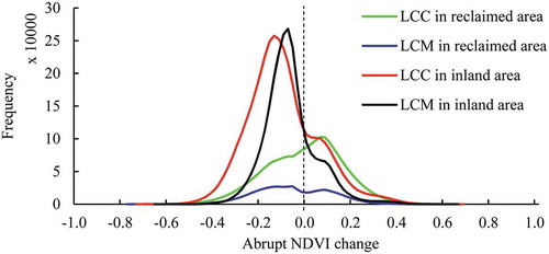
LCC and LCM reduced vegetation greenness by 68.2% and 75.0%, respectively (). LCC had a similar mean magnitude of NDVI change (−0.0603) to that of LCM (−0.0585) in Zhejiang’s coastal area. The conditions varied more between reclaimed and inland areas. In the reclaimed area, LCC had marginally positive effects (0.0036) on abrupt NDVI change, and LCM showed negative effects. In the inland area, both LCC and LCM had negative mean magnitudes of NDVI change. But not all land-cover changes resulted in decreased greenness. The frequency distribution of the magnitude of the NDVI change caused by LCC and LCM showed different patterns in the reclaimed and inland areas (). The patterns of LCC and LCM in the reclaimed area are much different, with the peak at 0.06 for LCC and very flat for LCM. Peaks of NDVI magnitudes in LCC and LCM occurred at −0.14 and −0.08 with similar shapes in the histogram.
Table 10. Mean NDVI change magnitude and proportion of negative NDVI change magnitude of abrupt change in the coastal area of Zhejiang Province, China.
Figure 7. Frequency (number of pixels) for varying magnitudes of abrupt NDVI change in China’s Zhejiang Province coastal area during 1986–2015.
In the reclaimed area, LCC in most land-cover types (mainly the types with low vegetation coverage) brought positive mean abrupt NDVI change (). Muddy tidal flats showed the highest positive NDVI magnitude of 0.0667. The high proportion (mostly larger than 65%) of positive NDVI change implied that most LCC increased vegetation greenness. In the inland area, most LCC showed negative mean NDVI change. Forest showed the largest change magnitude (−0.18) and had the highest proportion of negative NDVI change (95.2%) among all land-cover types. Most LCM in vegetation ecosystems showed negative mean NDVI change in reclaimed and inland areas. However, the change magnitude of NDVI was much smaller than that of LCC. For example, LCM in forest decreased vegetation greenness with the mean NDVI change magnitudes of −0.0639 and −0.0661 in reclaimed and inland areas, respectively, while the values for LCC in forest were −0.1937 and −0.18.
Table 11. Mean abrupt NDVI change and percentage of negative NDVI change of land-cover conversion and modification in China’s Zhejiang Province coastal area.
Discussion
Abrupt change refers to large magnitude changes which usually occur in a short time and can be detected by many Landsat time-series change detection algorithms (Zhu Citation2017). However, it should be noted that the detected abrupt changes might differ according to different algorithms and different change magnitude level definitions. Some methods can provide abrupt change caused by LCC, such as classification differencing, while other methods monitor abrupt change induced by LCM within one land-cover type (mostly forest) (Zhu Citation2017). In these studies of land-cover change, the abrupt change was mostly related to LCC (Lambin, Geist, and Lepers Citation2003; Lasanta and Vicente-Serrano Citation2012; Xu et al. Citation2016; Zhu et al. Citation2016; Li et al. Citation2017). According to this study, LCM accounts for 35.4% of the detected abrupt changes, indicating it should not be neglected in land-cover change studies, especially in forest, dryland, and wetland (herbaceous land) ecosystems. The optimal number of partitions and the position of the breakpoints are determined by minimizing the Bayesian information criterion among all possible partitioning schemes given by the RSS matrix. Therefore, we assumed the method was consistent in different land-cover changes and regions for LCC and LCM. A smaller shift might be a characteristic of LCM, because only modification occurred in these land-cover changes. According to our study, LCC was dominant in both reclaimed and inland areas, indicating the LCM detection rate did not significantly increase. Only forest showed a high proportion of LCM in the inland area. This also proved the method was robust in detection of LCM and LCC. In general, the differences in change magnitudes of NDVI in different LCMs and LCCs can be fully described.
After discriminating between LCC and LCM, understanding the causes of changes is more practical. The drivers of LCC can be determined through interpreting land-cover types before and after the change. The general direction of LCC was sea–muddy tidal flat–halophyte–aquaculture pond–cultivated land–construction land in the reclaimed areas of Zhejiang Province. The actual evolution process might be simplified and diverse due to unique leading industries in different regions. Market change and policy guidance also caused the mutual evolution among aquaculture pond, salt plants, and herbaceous land. In the inland area, population growth and economic development have accelerated the increase of built-up and paved areas. Forest mainly changed to dryland due to the implementation of the arable land balance policy (Li et al. Citation2017). A large proportion of LCM occurred in vegetation-dominated ecosystems, including herbaceous land, forest, and dryland. The invasion of new species, reduction of soil moisture and salinity, and extreme drought were the main drivers of herbaceous ecosystem modification (He et al. Citation2014). The environmental factors (such as soil moisture and salinity) changed with the increasing duration of reclamation and led to the vegetation succession process (Wu, Wu, and Xiao Citation2008; Wu Citation2011). In Zhejiang’s coastal area, the main drivers of forest disturbance were fire, select logging, and extreme climate events (drought and typhoon) (Seidl et al. Citation2011; Liu et al. Citation2017). The occurrences of fire concentrated around Tomb-Sweeping Day (about April 5th) and is an important issue for forest managers every year. The typhoon is a unique disturbance factor of the forest ecosystem in the coastal area and has induced a large area of forest disturbance (such as uprooting, snapping of stems, breakage, and defoliation). In agriculture-dominated ecosystems, anthropogenic activities including change of crop types and management are important concerns affecting dryland vegetation greenness. However, the specific change agent for LCM should be further quantified based on more local information and auxiliary data.
LCC led to slight increases in NDVI, while LCM had considerably negative effects on NDVI in reclaimed areas. The increased greenness of LCC was because many conversions were from non-vegetation to vegetation. That is why D. Li et al. (Citation2017) concluded land-cover change led to vegetation greenness in the reclaimed area of Hangzhou Bay, while LCM mostly occurred in the densely vegetated ecosystems. The herbaceous ecosystem showed the highest NDVI change magnitude among all land-cover types in the reclaimed area, and the negative NDVI change accounted for 67.3% of the LCM. This was mainly because of the vegetation succession with the increases in reclamation. For example, biomass increased from Suaeda glauca to Phragmites australis, then decreased to Tamarix chinensis/Imperata cylindrical (Wu, Wu, and Xiao Citation2008). Frequent high temperatures and salinity also contributed to the negative impact of LCM on vegetation growth (He et al. Citation2014). LCC had a greater impact on abrupt NDVI change than LCM in the inland area. Because the dominant LCCs were from dryland to construction land and from forest to dryland in the inland area, both induced substantial greenness decrease. Such a pattern was also noted in Guangzhou, which showed that LCC led the negative value of the mean abrupt enhanced vegetation index change (Zhu et al. Citation2016). Time-series NDVI change was used extensively to analyze vegetation greenness (Jong et al. Citation2012; Zhu et al. Citation2016). The negative effects of LCC such as urbanization can degrade vegetation greenness (Zhu et al. Citation2016), whereas positive LCC such as returning farmland to forest and grassland led to sustained vegetation growth (Hao et al. Citation2017). LCM studies were mostly focused on forest disturbance (Devries et al. Citation2015). In this study, three changes including seasonal change, gradual (trend) change, and abrupt change were considered by structure change detection method. NDVI shifts during abrupt change were calculated after segmentation and removed gradual and seasonal changes. Therefore, the non-linearity can be avoided in the NDVI shifts. This study further differenced the LCC and LCM in reclaimed area and inland area and quantified their respective impacts on NDVI change. Such a comprehensive NDVI change study is helpful for in-depth analysis of vegetation greenness.
Several uncertainties and limitations existed in this study that should be further considered. (1) An NDVI-based time-series model might not be suitable for all land-cover types and change agents. Multiple vegetation indexes and flexible time-series models may be used for better land-cover change detection. (2) LCM also includes the gradual changes over a long period. This study focused on abrupt changes occurring over short periods. To better understand the LCM impacts on vegetation ecosystems, the gradual changes should be further examined. (3) The details of the land-cover class definition are critical for LCC and LCM determination, because the fewer classes there are, the smaller the fraction of the breaks that are LCC. Therefore, it should be considered more carefully in different research needs and used data.
Conclusion
LCC and LCM are two aspects of land-cover change. Based on time-series Landsat NDVI data, abrupt change detection, land-cover classification, and conversion filters, these two aspects were acquired simultaneously with the overall accuracy of 90.0% in the coastal area of Zhejiang Province. The overall accuracies of 89.6% and 86.3% for abrupt change detection and land-cover classification, respectively, indicated the proposed method can provide fundamental support for land-cover change studies in a complex landscape. Approximately half (49.4%) of Zhejiang’s coastal area has experienced at least one abrupt change in the past 30 years. For these abrupt changes, LCM accounts for 35.4%, implying that LCM cannot be ignored in land-cover change studies. LCC was the main change agent (78.0%) in the reclaimed area, and the proportion of LCM reached 40.5% in the inland area.
LCC and LCM are strongly land-cover dependent. In the reclaimed area, LCC most often occurred at non-vegetation land-covers such as muddy tidal flats, construction land, and aquaculture ponds; and LCM occurred mostly in vegetation coverage including herbaceous land and Spartina alterniflora. In the inland area, both LCC and LCM were concentrated in forest and dryland ecosystems. Overall, LCC had a mean magnitude of NDVI change similar to that of LCM. However, LCC and LCM had positive and negative effects on NDVI change in the reclaimed area, but both had negative impacts on vegetation greenness in the inland area. Our results show the importance of taking both LCC and LCM into account when analyzing land-cover changes and their effects on vegetation greenness. They also demonstrate the importance of investigating reclaimed and inland areas separately.
Acknowledgements
We thank the United States Geological Survey (USGS) for providing long-term time-series Landsat surface reflectance products.
Disclosure statement
No potential conflict of interest was reported by the authors.
Additional information
Funding
References
- Alaibakhsh, M., I. Emelyanova, O. Barron, A. Mohyeddin, and M. Khiadani. 2015. “Multivariate Detection and Attribution of Land-Cover Changes in the Central Pilbara, Western Australia.” International Journal of Remote Sensing 36 (10): 2599–2621.
- Bai, J., and P. Perron. 1998. “Estimating and Testing Linear Models with Multiple Structural Changes.” Econometrica 66 (1): 47–78. doi:10.2307/2998540.
- Bai, J., and P. Perron. 2003. “Critical Values for Multiple Structural Change Tests.” The Econometrics Journal 6 (1): 72–88. doi:10.1111/1368-423X.00102.
- Breiman, L. 2001. “Using Iterated Bagging to Debias Regressions.” Machine Learning 45 (3): 261–277. doi:10.1023/A:1017934522171.
- Chowdhury, S., D. K. Chao, T. C. Shipman, and M. A. Wulder. 2017. “Utilization of Landsat Data to Quantify Land-Use and Land-Cover Changes Related to Oil and Gas Activities in West-Central Alberta from 2005 to 2013.” GIScience & Remote Sensing 54 (5): 700–720. doi:10.1080/15481603.2017.1317453.
- Cohen, W. B., Z. Q. Yang, and R. Kennedy. 2010. “Detecting Trends in Forest Disturbance and Recovery Using Yearly Landsat Time Series: 2. Timesync-Tools for Calibration and Validation.” Remote Sensing of Environment 114 (12): 2911–2924. doi:10.1016/j.rse.2010.07.010.
- Devries, B., M. Decuyper, J. Verbesselt, A. Zeileis, M. Herold, and S. Joseph. 2015. “Tracking Disturbance-Regrowth Dynamics in Tropical Forests Using Structural Change Detection and Landsat Time Series.” Remote Sensing of Environment 169: 320–334. doi:10.1016/j.rse.2015.08.020.
- Dutrieux, L. P., C. C. Jakovac, S. H. Latifah, and L. Kooistra. 2016. “Reconstructing Land Use History from Landsat Time-Series.” International Journal of Applied Earth Observation and Geoinformation 47: 112–124. doi:10.1016/j.jag.2015.11.018.
- Franklin, S. E., O. S. Ahmed, M. A. Wulder, J. C. White, T. Hermosilla, and N. C. Coops. 2015. “Large Area Mapping of Annual Land Cover Dynamics Using Multitemporal Change Detection and Classification of Landsat Time Series Data.” Canadian Journal of Remote Sensing 41 (4): 293–314. doi:10.1080/07038992.2015.1089401.
- Gómez, C., J. C. White, and M. A. Wulder. 2016. “Optical Remotely Sensed Time Series Data for Land Cover Classification: A Review.” Isprs Journal of Photogrammetry and Remote Sensing 116: 55–72. doi:10.1016/j.isprsjprs.2016.03.008.
- Hamunyela, E., J. Verbesselt, and M. Herold. 2016. “Using Spatial Context to Improve Early Detection of Deforestation from Landsat Time Series.” Remote Sensing of Environment 172: 126–138. doi:10.1016/j.rse.2015.11.006.
- Hansen, M. C., A. Egorov, P. V. Potapov, S. V. Stehman, A. Tyukavina, S. A. Turubanova, D. P. Roy, S. J. Goetz, T. R. Loveland, and J. Ju. 2014. “Monitoring Conterminous United States (Conus) Land Cover Change with Web-Enabled Landsat Data (Weld).” Remote Sensing of Environment 140 (1): 466–484. doi:10.1016/j.rse.2013.08.014.
- Hao, W., G. Liu, Z. Li, Y. Xin, B. Fu, and Y. H. Lü. 2017. “Analysis of the Driving Forces in Vegetation Variation in the Grain for Green Program Region, China.” Sustainability 9 (10): 1853. doi:10.3390/su9101853.
- He, B., Y. Cai, W. Ran, and H. Jiang. 2014. “Spatial and Seasonal Variations of Soil Salinity following Vegetation Restoration in Coastal Saline Land in Eastern China.” Catena 118: 147–153. doi:10.1016/j.catena.2014.02.007.
- Hermosilla, T., M. A. Wulder, J. C. White, N. C. Coops, G. W. Hobart, and L. B. Campbell. 2016. “Mass Data Processing of Time Series Landsat Imagery: Pixels to Data Products for Forest Monitoring.” International Journal of Digital Earth 9 (11): 1035–1054. doi:10.1080/17538947.2016.1187673.
- Hu, S., Z. Niu, Y. Chen, L. Li, and H. Zhang. 2017. “Global Wetlands: Potential Distribution, Wetland Loss, and Status.” Science of the Total Environment 586: 319–327. doi:10.1016/j.scitotenv.2017.02.001.
- Huang, C., S. N. Goward, J. G. Masek, N. Thomas, Z. Zhu, and J. E. Vogelmann. 2010. “An Automated Approach for Reconstructing Recent Forest Disturbance History Using Dense Landsat Time Series Stacks.” Remote Sensing of Environment 114 (1): 183–198. doi:10.1016/j.rse.2009.08.017.
- Huang, S., C. Ramirez, K. Kennedy, J. Mallory, J. Wang, and C. Chu. 2017. “Updating Land Cover Automatically Based on Change Detection Using Satellite Images: Case Study of National Forests in Southern California.” GIScience & Remote Sensing 54 (4): 495–514. doi:10.1080/15481603.2017.1286727.
- Jackson, R. D., and A. R. Huete. 1991. “Interpreting Vegetation Indices.” Preventive Veterinary Medicine 11 (3–4): 185–200. doi:10.1016/S0167-5877(05)80004-2.
- Jong, R. D., J. Verbesselt, M. E. Schaepman, and S. D. Bruin. 2012. “Trend Changes in Global Greening and Browning: Contribution of Short-Term Trends to Longer-Term Change.” Global Change Biology 18 (2): 642–655. doi:10.1111/j.1365-2486.2011.02578.x.
- Kennedy, R. E., Z. Yang, J. Braaten, C. Copass, N. Antonova, C. Jordan, and P. Nelson. 2015. “Attribution of Disturbance Change Agent from Landsat Time-Series in Support of Habitat Monitoring in the Puget Sound Region, USA.” Remote Sensing of Environment 166: 271–285. doi:10.1016/j.rse.2015.05.005.
- Kennedy, R. E., Z. Yang, W. B. Cohen, E. Pfaff, J. Braaten, and P. Nelson. 2012. “Spatial and Temporal Patterns of Forest Disturbance and Regrowth within the Area of the Northwest Forest Plan.” Remote Sensing of Environment 122 (4): 117–133. doi:10.1016/j.rse.2011.09.024.
- Kennedy, R. E., Z. Q. Yang, and W. B. Cohen. 2010. “Detecting Trends in Forest Disturbance and Recovery Using Yearly Landsat Time Series: 1. Landtrendr - Temporal Segmentation Algorithms.” Remote Sensing of Environment 114 (12): 2897–2910. doi:10.1016/j.rse.2010.07.008.
- Lambin, E. F., H. J. Geist, and E. Lepers. 2003. “Dynamics of Land-Use and Land-Cover Change in Tropical Regions.” Annual Review of Environment and Resources 28 (28): 205–241. doi:10.1146/annurev.energy.28.050302.105459.
- Lasanta, T., and S. M. Vicente-Serrano. 2012. “Complex Land Cover Change Processes in Semiarid Mediterranean Regions: An Approach Using Landsat Images in Northeast Spain.” Remote Sensing of Environment 124 (6): 1–14. doi:10.1016/j.rse.2012.04.023.
- Li, D., D. Lu, M. Wu, X. Shao, and J. Wei. 2017. “Examining Land Cover and Greenness Dynamics in Hangzhou Bay in 1985–2016 Using Landsat Time-Series Data.” Remote Sensing 10 (1): 32. doi:10.3390/rs10010032.
- Li, J., M. Ye, R. Pu, Y. Liu, Q. Guo, B. Feng, R. Huang, and G. He. 2018. “Spatiotemporal Change Patterns of Coastlines in Zhejiang Province, China, over the Last Twenty-Five Years.” Sustainability 10 (2): 477. doi:10.3390/su10020477.
- Liu, S., X. Wei, D. Li, and D. Lu. 2017. “Examining Forest Disturbance and Recovery in the Subtropical Forest Region of Zhejiang Province Using Landsat Time-Series Data.” Remote Sensing 9 (5): 479. doi:10.3390/rs9050479.
- Lu, D., G. Li, and E. Moran. 2014. “Current Situation and Needs of Change Detection Techniques.” International Journal of Image and Data Fusion 5 (1): 13–38. doi:10.1080/19479832.2013.868372.
- Lu, D., P. Mausel, E. Brondizio, and E. Moran. 2004. “Change Detection Techniques.” International Journal of Remote Sensing 25 (12): 2365–2401. doi:10.1080/0143116031000139863.
- Masek, J. G., and G. J. Collatz. 2006. “Estimating Forest Carbon Fluxes in a Disturbed Southeastern Landscape: Integration of Remote Sensing, Forest Inventory, and Biogeochemical Modeling.” Journal of Geophysical Research 111 (G1): 670–674. doi:10.1029/2005JG000062.
- Parmentier, B. 2014. “Characterization of Land Transitions Patterns from Multivariate Time Series Using Seasonal Trend Analysis and Principal Component Analysis.” Remote Sensing 6 (12): 12639–12665. doi:10.3390/rs61212639.
- Peneva-Reed, E. 2014. “Understanding Land-Cover Change Dynamics of a Mangrove Ecosystem at the Village Level in Krabi Province, Thailand, Using Landsat Data.” GIScience & Remote Sensing 51 (4): 403–426. doi:10.1080/15481603.2014.936669.
- Schultz, M., J. G. P. W. Clevers, S. Carter, J. Verbesselt, V. Avitabile, H. V. Quang, and M. Herold. 2016. “Performance of Vegetation Indices from Landsat Time Series in Deforestation Monitoring.” International Journal of Applied Earth Observation and Geoinformation 52: 318–327. doi:10.1016/j.jag.2016.06.020.
- Seidl, R., P. M. Fernandes, T. F. Fonseca, F. O. Gillet, A. M. Jönsson, K. Merganičová, S. Netherer, et al. 2011. “Modelling Natural Disturbances in Forest Ecosystems: A Review.” Ecological Modelling 222 (4): 903–924. doi:10.1016/j.ecolmodel.2010.09.040.
- Shi, Z., R. Wang, M. Huang, and D. Landgraf. 2002. “Detection of Coastal Saline Land Uses with Multi-Temporal Landsat Images in Shangyu City, China.” Environmental Management 30 (1): 142–150. doi:10.1007/s00267-001-2645-8.
- Shih, H. C., D. A. Stow, J. R. Weeks, and L. L. Coulter. 2017. “Determining the Type and Starting Time of Land Cover and Land Use Change in Southern Ghana Based on Discrete Analysis of Dense Landsat Image Time Series.” IEEE Journal of Selected Topics in Applied Earth Observations & Remote Sensing 9 (5): 2064–2073. doi:10.1109/JSTARS.2015.2504371.
- Shimizu, K., O. S. Ahmed, R. Ponce-Hernandez, T. Ota, Z. C. Win, N. Mizoue, and S. Yoshida. 2017. “Attribution of Disturbance Agents to Forest Change Using a Landsat Time Series in Tropical Seasonal Forests in the Bago Mountains, Myanmar.” Forests 8 (6): 218. doi:10.3390/f8060218.
- Turner, B. L. I., D. L. Skole, S. Sanderson, G. Fischer, L. Fresco, and R. Leemans. 1995. “Land-Use and Land-Cover Change. Science/Research Plan.” Global Change Report 43 (1995): 669–679.
- Verbesselt, J., R. Hyndman, G. Newnham, and D. Culvenor. 2010. “Detecting Trend and Seasonal Changes in Satellite Image Time Series.” Remote Sensing of Environment 114 (1): 106–115. doi:10.1016/j.rse.2009.08.014.
- Wang, W., H. Liu, Y. Li, and J. Su. 2014. “Development and Management of Land Reclamation in China.” Ocean & Coastal Management 102: 415–425. doi:10.1016/j.ocecoaman.2014.03.009.
- Wang, X., Y. Liu, F. Ling, Y. Liu, and F. Fang. 2017. “Spatio-Temporal Change Detection of Ningbo Coastline Using Landsat Time-Series Images during 1976–2015.” ISPRS International Journal of Geo-Information 6 (3): 68. doi:10.3390/ijgi6030068.
- Wu, T. 2011. “Plant Distribution in Relation to Soil Conditions in Hangzhou Bay Coastal Wetlands, China.” Pakistan Journal of Botany 43 (43): 2331–2335.
- Wu, T. G., M. Wu, and J. H. Xiao. 2008. “Dynamics of Community Succession and Species Diversity of Vegetations in Beach Wetlands of Hangzhou Bay.” Chinese Journal of Ecology 27 (8): 1284–1299.
- Xu, L., B. Li, Y. Yuan, X. Gao, T. Zhang, and Q. Sun. 2016. “Detecting Different Types of Directional Land Cover Changes Using Modis NDVI Time Series Dataset.” Remote Sensing 8 (6): 495. doi:10.3390/rs8060495.
- Zeileis, A., C. Kleiber, W. Krämer, and K. Hornik. 2003. “Testing and Dating of Structural Changes in Practice.” Computational Statistics & Data Analysis 44 (1): 109–123. doi:10.1016/S0167-9473(03)00030-6.
- Zhu, Z. 2017. “Change Detection Using Landsat Time Series: A Review of Frequencies, Preprocessing, Algorithms, and Applications.” ISPRS Journal of Photogrammetry and Remote Sensing 130: 370–384. doi:10.1016/j.isprsjprs.2017.06.013.
- Zhu, Z., and C. E. Woodcock. 2014. “Continuous Change Detection and Classification of Land Cover Using All Available Landsat Data.” Remote Sensing of Environment 144: 152–171. doi:10.1016/j.rse.2014.01.011.
- Zhu, Z., Y. Fu, C. E. Woodcock, P. Olofsson, J. E. Vogelmann, C. Holden, M. Wang, S. Dai, and Y. Yu. 2016. “Including Land Cover Change in Analysis of Greenness Trends Using All Available Landsat 5, 7, and 8 Images: A Case Study from Guangzhou, China (2000–2014).” Remote Sensing of Environment 185: 243–257. doi:10.1016/j.rse.2016.03.036.
- Zscheischler, J., M. D. Mahecha, S. Harmeling, and M. Reichstein. 2013. “Detection and Attribution of Large Spatiotemporal Extreme Events in Earth Observation Data.” Ecological Informatics 15 (2): 66–73. doi:10.1016/j.ecoinf.2013.03.004.