Unsupervised evaluation-based region merging for high resolution remote sensing image segmentation

Abstract

Image segmentation has a remarkable influence on the classification accuracy of object-based image analysis. Accordingly, how to raise the performance of remote sensing image segmentation is a key issue. However, this is challenging, primarily because it is difficult to avoid over-segmentation errors (OSE) and under-segmentation errors (USE). To solve this problem, this article presents a new segmentation technique by fusing a region merging method with an unsupervised segmentation evaluation technique called under- and over-segmentation aware (UOA), which is improved by using edge information. Edge information is also used to construct the merging criterion of the proposed approach. To validate the new segmentation scheme, five scenes of high resolution images acquired by Gaofen-2 and Ziyuan-3 multispectral sensors are chosen for the experiment. Quantitative evaluation metrics are employed in the experiment. Results indicate that the proposed algorithm obtains the lowest total error (TE) values for all test images (0.3791, 0.1434, 0.7601, 0.7569, 0.3169 for the first, second, third, fourth, fifth image, respectively; these values are averagely 0.1139 lower than the counterparts of the other methods), as compared to six state-of-the-art region merging-based segmentation approaches, including hybrid region merging, hierarchical segmentation, scale-variable region merging, size-constrained region merging with edge penalty, region merging guided by priority, and region merging combined with the original UOA. Moreover, the performance of the proposed method is better for artificial-object-dominant scenes than the ones mainly covering natural geo-objects.

Keywords:

• image segmentation
• high resolution remote sensing image
• unsupervised evaluation
• over- and under-segmentation aware
• region merging

1. Introduction

With the rapid development of remote sensing technology, the quantity of earth-observation image data is increasing at an amazing speed, giving rise to the era of geo-spatial big data (Li et al. 2016; Cai, Huang, and Song 2017). How to accurately and efficiently extract geo-information from such a huge and growing dataset becomes a stringent need (Guo 2018) and a difficult issue (Liu et al. 2016). Object-based image analysis (OBIA), which has received considerable attention in remote sensing community (Blaschke 2010; Blaschke et al. 2014; Chen and Weng 2018), provides a promising solution (Chen et al. 2018). The main advantage of OBIA is to use region/segment-based features, equipping the process of geo-object recognition with high-level semantic knowledge. Image segmentation is usually deemed as the first step in OBIA, and produces a significant impact on classification accuracy. Although there is a large body of literature about image segmentation, it is still challenging to produce high-quality segmentation results for various remotely sensed images (Costa, Foody, and Boyd 2018).

Previous studies on remote sensing image segmentation can be roughly divided into two groups: top-down and bottom-up. The former achieves the partition of an image by iteratively splitting the whole scene into small and homogeneous regions. Quad-tree-based technique (Finkel and Bentley 1974; Wu, Hong, and Rosenfeld 1982) is an example. In the beginning, the entire image is divided as four rectangular segments. Then, each segment is iteratively divided if its homogeneity is not high enough. Although it is efficient, it cannot guarantee that the shape of each geo-object can be delineated accurately. To solve this problem, Fu et al. (2013) added a region merging process into quad-tree segmentation, so that some over-segmented regions can be completely extracted. However, it may suffer from imbalanced merging, i.e., if a merging should occur for a large segment and a very small one, it may not be enforced, since the large discrepancy in size leads to a difference in low-level features (geometric, spectral and textural).

Due to the factors mentioned above, more researchers prefer bottom-up strategies. In this category, a very prevalent type is region merging. Many methods, such as hierarchical step-wise optimization (Beaulieu and Goldberg 1989), seeded region growing (Adams and Bischof 1994), segmentation engine (Gofman 2006), size-constrained region merging (Castilla, Hay, and Ruiz 2008), iterative region growing using semantics (Yu and Clausi 2008; Qin and Clausi 2010), hierarchical segmentation (HSEG) (Tilton et al. 2012; Tilton and Passoli 2014), binary partition tree (Valero, Salembier, and Chanussot 2013; Salembier and Foucher 2016; Su and Zhang 2018), tile-based region merging (Lassalle et al. 2015), scale-variable region merging (Yang, He, and Caspersen 2017), are based on this technique.

Among the aforementioned approaches, a popular one is a multi-resolution segmentation (MRS) (Baatz and Schäpe 2000), which has been commercially available in the Definiens developer platform and has been employed in many land-cover mapping applications (Vieira et al. 2012; Kim and Yeom 2014; Yu et al. 2016). Several variants of MRS were proposed. For example, Zhang et al. (2013) developed a boundary-constrained region merging based on spectral and edge features. Yu et al. (2013) also improved merging criterion by using spectral, edge and textural features. Chen, Qiu, and Wu (2015) proposed a similar approach, the merging criterion of which includes a constraint on segment size. Su (2017a) established a three-stage segmentation algorithm. Although these modifications are able to enhance segmentation quality, how to end region merging process remains a difficult issue. In most cases, the termination of region merging is controlled by a single/fixed scale threshold. Larger/smaller scale tends to produce more/less merging, and under/over-segmentation error (USE/OSE) may occur. For large images, in which a globally optimal scale can be hardly adapted to some local parts, unsatisfactory results may be locally yielded. To solve this problem, Yang, He, and Caspersen (2017) proposed a scale variable scheme. Although this method is effective to produce various-sized segments, its adaptability for complicated scenes is limited.

Another direction to improve region merging focuses on merging order. The basic idea is to prioritize appropriate merging. An example is hybrid region merging (HRM) (Zhang et al. 2014), which alternatively uses local and global mutual best fitting rule to identify the merging to be executed. In addition, an exploration was made by Su (2017b), who proposed a scheme called region merging guided by priority (RMGP).

According to the aforementioned studies, in order to increase segmentation accuracy, OSE and USE should be reduced simultaneously. To achieve this goal, previous studies all tried to improve merging criterion or merging order by using various spectral and/or spatial features. These efforts can be deemed as indirect to reduce OSE and USE, since the two types of segmentation error are not explicitly formulated. In fact, if the information of segmentation error type can be explicitly utilized in a region merging process, it is likely to enhance segmentation quality. The reasons are two-fold. (1) An OSE can be removed if s segment only covering a part of a geo-object is merged. Such a segment can be deemed as OSE. (2) A USE can be prevented if a segment which fully represents the shape of a geo-object is not merged. Such a segment is possibly considered as not having any types of segmentation error. Accordingly, it is safe to hypothesize that segmentation accuracy can be raised if a region merging process is aware of the segmentation error type. To implement such an approach, a straightforward way is to combine a segmentation evaluation technique with region merging. This work is motivated by this idea. But before introducing its details, some information about segmentation evaluation strategies is worth mentioning.

In general, segmentation evaluation strategies can be coarsely divided into two groups: supervized and unsupervised (Marpu et al. 2010; Su and Zhang 2017). The former type requires ground truth, the production of which is subjective and labor-intensive. However, when good ground truth segmentation is available, supervised evaluation metrics can yield better results than unsupervised methods. But, when ground truth data are unavailable, unsupervised metrics can help produce optimal segmentation result. This is achieved by selecting the optimal segmentation parameter(s). An example is to determine the optimal scale parameter for MRS and many efforts have been published. For instance, Johnson and Xie (2011) adopted area weighted variance and global Moran’s index to identify the optimal scale for MRS. They assumed that with the increase of scale, area weighted variance of all segments climbs up while neighboring segments’ spatial correlation decreases. A goodness score was designed to quantify this pattern. The scale with the lowest goodness score is considered optimal. Böck, Immitzer, and Atzberger (2017) improved this method from the aspect of numerical behavior. Similar studies were reported by Yang, Li, and He (2014) and (2015)). Although these methods can automate MRS and MRS-like methods, they cannot explicitly identify OSE/USE.

To overcome the aforementioned limitation, a recently proposed unsupervised evaluation technique, called under- and over-segmentation aware (UOA) (Troya-Galvis et al. 2015), provides a solution, since it can explicitly identify OSE/USE for each segment. What’s more, to estimate the segmentation error type of one segment, UOA only needs the input of this segment and its neighboring ones. This is different from the goodness score-based methods, which take all of the segments as input. In this way, by using UOA, it is possible to enable the identification of segmentation error type during the region merging process. Su (2018) mentioned that there is a defect in the OSE estimation of the UOA originally proposed by Troya-Galvis et al. (2015). Thus, an improved version of UOA was proposed to enhance its evaluation performance. Inspired by these features, UOA is fused with a region merging method, which can be considered as the most important contribution of this article. In doing so, over-segmented segments/regions are prioritized for merging and others are stopped from merging. In this way, OSE and USE can be reduced. Since there is a defect in the OSE estimation of the original UOA, this metric is improved by using an edge feature. In addition, a new edge-based merging criterion is developed to further enhance segmentation performance. Since the aforementioned contributions of this study are both associated with edge information, it is necessary to brief previous works related to this type of image feature.

A large number of remote sensing image segmentation algorithms use edge information, and their schemes of using edge-related features can be broadly divided into two categories. The first category merely considers edge strength in the construction of merging criterion or merging order, such as the methods developed by Zhang et al. (2013), Yu et al. (2013), and Su (2017a, 2017b). The second category utilizes edge information to determine the optimal segmentation parameter(s). A recently proposed scale estimation model (Liu et al. 2018) based on vector edge is a typical example of this category. Moreover, Chen et al. (2014) optimized MRS by using common-boundary edge information, which is not only used in its merging criterion, but also in its scale determination procedure. However, in their method, the scale determination process is executed prior to its region merging process, which is the major difference to the algorithm proposed in this work.

This paper is organized as follows. Section 2 presents the principle of the proposed approach. Experimental results are detailed in section 3, followed by discussions on the advantages and limitations of the proposed algorithm. Concluding remarks are in the last section. For the convenience of reading, Table 1 lists the acronyms for the important terms adopted in this paper.

Table 1. Acronyms for the important terms used in this paper. They are listed alphabetically.

Acronym	Full name
GMBF	Global mutual best fitting
GOSE	Global over segmentation error
GUSE	Global under-segmentation error
HRM	Hybrid region merging
IUOAS	Improved under- and over-segmentation aware segmentation
LMBF	Local mutual best fitting
MRS	Multi-resolution segmentation
OBIA	Object-based image analysis
OSE	Over segmentation
OUOAS	Original under- and over-segmentation aware segmentation
RMGP	Region merging guided by priority
SCEP	Size constrained region merging with edge penalty
SP	Scale parameter
SVRM	Scale variable region merging
TE	Total error
UOA	Under and over-segmentation aware
USE	Under-segmentation error

2. Methodology

There are two main contributions to the proposed method. (1) The original under- and over-segmentation aware (UOA) is improved by using edge information, and it is fused with a region merging technique. This strategy aims at enforcing potentially correct merging. Note that the improved UOA was initially proposed in our previous work published as a conference paper (Su 2018), while in this paper, the main contribution resides in that the improved UOA is fused with a region merging approach. Accordingly, this paper can be deemed as an extension of our previous work. (2) An edge-based merging criterion is developed to increase segmentation accuracy. Although some previous studies also adopted edge information, most of them only utilized edge information at the common boundary pixels of two candidate segments. The proposed metric uses the edge information of all boundary pixels, so that the new criterion can favor the merging of the segments which are incompletely extracted.

Figure 1 illustrates the relationship between the contributions and the objective of this study. It is evident to see that edge strength plays a key role in the proposed methodology, since the two main contributions both rely on this type of information. Note that the two contributions help achieve the research goal from different angles, which will be detailed in the following.

Figure 1. Relationship of the two main contributions.

2.1. The proposed segmentation method

The new region merging technique has three stages: (1) identify the error type of each segment by using the improved UOA; (2) determine the merging order by using the global mutual best fitting (GMBF) rule; (3) do region merging according to the sequence produced at stage (2). In the implementation of stage (1), all of the segments have a feature variable represented by E_δ, which is estimated by using UOA. The estimation of E_δ is detailed in sub-section 2.2, and its value indicates the segmentation error type of a segment. Based on this, the segments which have an under-segmentation error (USE) or no error is stopped from merging, but those having an over-segmentation error (OSE) are considered for merging. In this way, UOA is fused with region merging. Note that this is the most important contribution of this paper.

The overall process of the proposed segmentation algorithm is detailed in Table 2. n_merging is used as a flag for termination. It is important to note that, in step 4, how to determine the order of merging is detailed in sub-section 2.3. Such a criterion indicates the appropriateness for merging a pair of segments. Another important thing in step 4 is that each element in list contains three variables: two neighboring segments and their appropriateness for merging. To save memory, the variable representing each segment is a pointer. Furthermore, all of the elements in list are arranged in ascending order according to appropriateness value, meaning that the pair of segments in the first element is the most suitable for merging. To construct list, a greedy search is implemented. In this process, all of the segments are visited in a one by one sequence. For each segment, local mutual best fitting rule (LMBF) (Baatz and Schäpe 2000) is used to find its most appropriate neighbor for merging. The merging order derived by using list and LMBF is equivalent to GMBF (Baatz and Schäpe 2000). In step 4, it is also crucial to note that for an element in the list, if the segmentation error type of either one of the two segments is not OSE, the element will be excluded from list. In this way, some potential USEs can be avoided.

Table 2. Implementation details of the proposed region merging approach.

Input: image; edge strength map; parameter δ and γ; shape and compactness coefficients Output: segmentation result

1. Initialize each pixel as a single segment; 2. Estimate Eδ for each segment; 3. Set the count of merging variable nmerging as 0; 4. Determine the merging order and store it in a list; 5. Merge segments according to the sequence of list; after each merging, increase nmerging by 1 and remove the corresponding element in list; this process is iterated until the list is empty; 6. If nmerging > 0, go back to step 2; otherwise finish the process and output result.

To better illustrate the proposed technique, Figure 2 provides a flowchart, which unveils how the two contributions act. It is clear that the improved UOA directly influences the region merging process. Since region merging is a bottom-up procedure, it is critical to avoid merging the segments with USE. Fusing region merging with UOA is a straightforward way to achieve this goal. By using the improved UOA, the error type of each segment is expected to be more accurately identified, so that segmentation quality can be enhanced.

Figure 2. Flowchart of the proposed algorithm.

Independent of the first contribution, contribution (2) aims at penalizing the inappropriate merging by using a new edge-based merging criterion. This method utilizes the edge strength of all boundary pixels of a segment, so that the boundary completeness of a segment can be delineated. If a segment has a high degree of edge completeness, the fitness value measured by Equation (4) should be high. In this way, inappropriate merging can be constrained.

2.2 The improved UOA

This work is an extension of our previous work published in a conference paper (Su 2018), in which the improved UOA was initially proposed. For better understanding the mechanism of the proposed segmentation approach, the principle of the improved UOA is only briefly introduced in this sub-section, readers are referred to (Su 2018) for more details for the improved UOA.

In a segmentation result of a remote sensing image, the original UOA locally identifies the segmentation error type for a segment S_i by using:

(1) $E_{\delta }\left(S_i\right)=\left\{\begin{array}{c}-1\\ 1\\ 0\end{array}\begin{array}{c}\mathrm{i}\mathrm{f}H\left(S_i\right)>\delta \\ \mathrm{i}\mathrm{f}H\left(S_i\right)<\delta \mathrm{a}\mathrm{n}\mathrm{d}\mathrm{\exists }{S}_j\in N\left(S_i\right)\wedge H\left(S_i\cup S_j\right)<\delta \\ \mathrm{o}\mathrm{t}\mathrm{h}\mathrm{e}\mathrm{r}\mathrm{w}\mathrm{i}\mathrm{s}\mathrm{e}\end{array}\right.$(1)

where E_δ(S_i) represents the segmentation error type of segment S_i, and it indicates USE, OSE, or not an error when it is valued as −1, 1, 0, respectively; H(·) is heterogeneity measure which can be simply formulated by using intra-segment heterogeneity (Troya-Galvis et al. 2015); δ is a heterogeneity threshold, and if H(S_i) > δ, S_i is considered to be too heterogeneous; N(S_i) means a set of segments that are neighbors of S_i.

As mentioned in the previous study (Su 2018), there is a defect in the OSE detection of the original UOA. To overcome this problem, edge information is added to the second line of the right part of Equation (1). If S_i is homogeneous enough (H(S_i) < δ), then find all of its neighbors which meet H(S_i∪S_j) < δ, and add these segments into a set N_H. Subsequently, if one of N_H’s element S_j has weak edge strength at the common boundary with S_i, then E_δ(S_i) = 1. In implementation, the key issue is to identify a weak edge at the common boundary between two segments. Two steps are designed as a solution. First, an edge strength map whose pixel values are within the scope of [0,1], is generated. Second, Equation (2) is exploited to detect weak edge:

(2) $M_{\mathrm{E}\mathrm{S}}\left(S_i,S_j\right)=\left\{\begin{array}{c}1\mathrm{i}\mathrm{f}\left(1/\left|C\left(S_i,S_j\right)\right|\right)\hspace{0.17em}\hspace{0.17em}\sum C_{\mathrm{E}\mathrm{S}}\left(S_i,S_j\right)<\hspace{0.17em}\gamma \\ 0\mathrm{o}\mathrm{t}\mathrm{h}\mathrm{e}\mathrm{r}\mathrm{w}\mathrm{i}\mathrm{s}\mathrm{e}\end{array}\right.$(2)

where M_ES(S_i,S_j) is weak edge indicator, if it equals 1, there exists a weak boundary between two neighboring segments; C(S_i,S_j) represents a set of pixels at the common boundary of the segments S_i and S_j, and |C(S_i,S_j)| is the boundary length; C_ES(S_i,S_j) is the value of a pixel belonging to C(S_i,S_j); γ is a threshold. Higher γ tends to yield more weak edges.

According to the above description, there are totally two parameters in the improved UOA: δ and γ. Their numerical ranges are both (0,1). These two parameters are thus introduced in the proposed segmentation algorithm, and their effects on the segmentation performance should be analyzed.

2.3. The new merging criterion

The merging criterion used in the proposed algorithm is based on two parts: (1) heterogeneity change (Baatz and Schäpe 2000) and (2) edge strength information. Part (1) is adopted by the multi-resolution segmentation (MRS), which is embedded in the well-known eCognition developer platform. The two parameters (shape and compactness coefficient, marked as S and C in the following) in heterogeneity change are included in the proposed method. The two coefficients balance the contribution of spectra/geometry (S) and compactness/smoothness (C) to the value of total heterogeneity change. By default, S and C are, respectively, set as 0.1 and 0.5, and this setup is used throughout the experiment of this paper, because (1) they are found to perform sufficiently well, and (2) since they are fixed, the effects of the new merging criterion can be better analyzed.

In the new merging criterion, edge strength is added to the heterogeneity change, which has the following form:

(3) $\mathrm{\Delta }{H}_{\mathrm{n}\mathrm{e}\mathrm{w}}\left(S_1,S_2\right)=H\left(S_1,S_2\right)/\left(1-E_{\mathrm{c}}\left(S_1,S_2\right)\right)$(3)

where ΔH_new represents the new merging criterion; S₁ and S₂ symbolizes two adjacent segments; the brackets (S₁, S₂) in Equation (3) all indicate that the variable is calculated for segments S₁ and S₂; ΔH is the heterogeneity change measure; E_c is the maximal value of S₁’s and S₂’s edge completeness, which is calculated by:

(4) $E_{\mathrm{c}}\left(S_1,S_2\right)=\mathrm{m}\mathrm{a}\mathrm{x}\left(C_1,C_2\right)$(4)

where C₁ indicates the edge completeness of S₁, and C₂ is similarly defined. This variable is computed by:

(5) $C_1=\sum \mathrm{B}\mathrm{D}{\mathrm{R}}_{\mathrm{E}\mathrm{S}}\left(S_1\right)/P_1$(5)

where ΣBDR_ES(S₁) means the sum of all of the boundary pixels of S₁, and the pixel values are all derived from an edge strength map; P₁ is the perimeter length of S₁. In the proposed method, for the convenience of implementation, it is prescribed that the pixel value of the edge strength map ranges from 0 to 1. Accordingly, it can be seen that C₁ has the numerical range of (0,1].

From Equations (3) and (5), it can be understood that the edge information serves as a penalty term for the merging criterion. The explanation is as follows. For any segment, if it is already a good approximation of a real geo-object, its edge completeness is supposed to be very near to 1, and thus the ΔH_new will be much higher than ΔH, constraining the merging with such a segment.

By using the new merging criterion, some erroneous merging can be avoided, so that some large segments covering several different geo-objects can be reduced, i.e., USE can be diminished. Because according to Equation (4), the appropriateness to merge well-developed segments is penalized, and thus the chance of erroneous merging can be decreased, leading to the reduction of USE.

3. Experiment and results

3.1. Dataset

To fully test the proposed approach, five scenes of high resolution multi-spectral images were adopted for experiment. The first four images can be seen in Figure 3. The first one is termed as T1. It captures an urban area, and mainly contains roof tops and roads. This scene was derived by GaoFen-2, a Chinese remote sensing satellite with high spatial resolution. The second image (coded as T2) which is primarily composed of aqua-cultural pools, displays a rural area. T2 was obtained by ZiYuan-3, which is also a Chinese satellite designed for land resources observation. T1 and T2 are both dominated by artificial geo-objects, which makes them similar in geo-physical appearance. To fully test the robustness of the proposed algorithm, two more different images are collected. The third image, termed as T3, covers a mountainous area. Since the local place has a high altitude and a warm climate, snowy and vegetative hills coexist, leading to a unique landscape. The last image, with code name T4, is rich in vegetation and wetlands, such as small lakes and narrow rivers. As can be observed from Figure 3, natural geo-objects pervade T3 and T4, which distinguishes them from T1 and T2.

Figure 3. The dataset used for the experiment. (a) to (d) show the false-color (R: Near-infrared, G: Red, B: Green) image of T1, T2, T3, T4, respectively. (e) to (h) are the reference segments of T1, T2, T3, T4, respectively. (i) to (l) display edge strength maps for T1, T2, T3, T4, respectively.

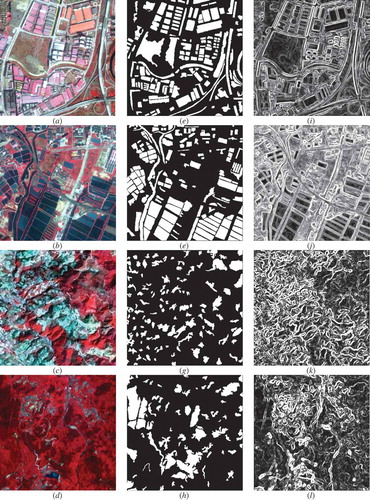
The four images all have a size of 400 × 400 pixels, and their basic information can be seen in Table 3. They all contain four spectral channels: near-infrared, red, green and blue, and the first three bands are used in this work, because it was found that the blue channel had relatively small effects on the segmentation performance and it increases the computational burden. Some related results are provided in sub-section 3.3.

Table 3. Details of the four images used for the experiment.

Number	Platform	Spatial Resolution	Central coordinate	Location	Acquisition date
T1	GaoFen-2	4.0 meter	E114°9′17″, N30°35′3″	Wuhan city, Hubei province, China	12 February 2015
T2	ZiYuan-3	5.8 meter	E113°44′8″, N22°46′24″	Dongguan city, Guangdong province, China	23 December 2013
T3	GaoFen-2	4.0 meter	E99°51′14″, N22°32′41″	Xishuangbanna Daizu county, Yunnan province, China	25 January 2014
T4	ZiYuan-3	5.8 meter	E119°21′16″, N25°47′8″	Fuqing county, Fujian province, China	16 April 2014

Pre-processing for the four images only includes the atmospheric correction. Geometric correction is not performed since it was finished by the vendor. FLAASH tool embedded in ENVI software is used for the pre-processing. The default parameters are adopted, because this setting is found to perform sufficiently well for this experiment. Cloud coverage of the four images is all below 1%.

In order to precisely and quantitatively validate the performance of the proposed technique, reference segmentations for some representative geo-objects in the dataset are prepared. They are manually extracted as polygons by three expert interpreters. In this process, for each test image, one expert produces one manual segmentation result, leading to three different results for each image. To ensure quality, the three different results of the same scene are cross-checked to eliminate unreliable or inaccurate polygons. As a result, 152, 144, 116, 72 reference polygons are adopted for T1, T2, T3, T4, respectively. They can be seen as the white polygons in the middle column of Figure 3, and it can be observed that they well embody the geometric information of their corresponding geo-objects.

Since the improved UOA and the new merging criterion require an edge strength map, the method developed by (Devereux, Amable, and Posada 2004) is employed to produce it. This method was reported to be effective (Su 2017b). The right column of Figure 3 exhibits the results. The white pixels indicate strong edge signature while the black ones have the opposite meaning. It can be seen from these sub-figures that the white pixels agree well with the boundaries of major geo-objects.

3.2. Validation of the improved UOA

Although the improved UOA has been validated in our previous research (Su 2018), it is still necessary to validate it by using the dataset of this study, since it directly affects the performance of the proposed segmentation technique. For this purpose, hybrid region merging (HRM) is exploited to yield a series of segmentation results. There are totally three parameters in HRM, shape and compactness coefficients and scale. The former two are fixed at 0.1 and 0.5, respectively, and scale varies from 10 to 200 with 10 as the incremental step, leading to 20 different segmentation results. These results are subsequently input into the original and the new UOA approaches, to see if the defect of the original UOA is alleviated. Note that only the results of T1 are displayed, because the counterparts of the other images are quite similar.

Before analyzing the evaluation results of the two UOA methods, it is necessary to understand the quality of the 20 segmentation results. For this purpose, supervised evaluation scores (global over segmentation error, GOSE, and global under-segmentation error, GUSE) computed by using a recently developed method (Su and Zhang 2017) are plotted against scale (Figure 4(a)). Its primary advantage is that OSE and USE can be independently quantified, when the two types of segmentation error coexist (Su and Zhang 2017). Since in most real-world image segmentation problems, OSEs and USEs often appear at the same time, this approach can reliably quantify the degree of the two types of segmentation incorrectness. In this experiment, in order to demonstrate the effects of the proposed UOA method, it is necessary to observe the evaluation result of the improved UOA for different types of segmentation. Su and Zhang’s method provides an explicit reference evaluation result for different types of segmentation, which helps understand the performance of the proposed UOA.

Figure 4. Analytical results for validating the improved UOA. (a) Relationship between the supervised evaluation scores (GOSE, GUSE and TE) and scale parameter. (b) The relationship between γ and θ.

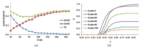
According to Figure 4(a), it can be seen that when scale is lower than 50, OSE is very dominant but USE is quite small. As scale climbs up, OSE decreases while USE becomes more serious. Such results are quite consistent with previous studies (Grybas, Melendy, and Congalton 2017; Liu, Du, and Mao 2017; Liu and Xia 2010). Note that the TE metric in Figure 4(a) is the sum of GOSE and GUSE, and it will be discussed in the next sub-section.

Considering that the improved UOA is only different from the old one in terms of estimating OSE, thus θ (Troya-Galvis et al. 2015), which is used by the original UOA to reflect total OSE, is plotted against the different scale and threshold γ. This analysis aims at unveiling the effect of γ, which is directly related to the improvement of the new UOA. Figure 4(b) exhibits these results. Note that δ is fixed at 0.5. It is also necessary to address that the curves of scale 10 and 20 are very similar, thus the results of scale 5 are generated and used in Figure 4(b). From this sub-figure, it can be observed that when γ is less than 0.3, most curves are overlapped with the horizontal axis. Additionally, it is interesting to note that with the increase of γ, θ becomes larger for all of the scales, because according to Equation (3), larger γ allows more common boundaries to be determined as weak edges, making more regions identified as containing OSE. Another interesting phenomenon is that θ is higher for small scales, since OSE is inherently more dominant when the scale is low. Aside from the aforementioned observations, an important finding is that for all scales, θ curves have very high increasing rate for γ at intermediate values (generally between 0.3 and 0.6, but such numerical range may vary slightly for different scales), reflecting that the OSE estimation of the improved UOA can be very sensitive to γ when this parameter is between 0.3 and 0.6, thus care should be taken for γ.

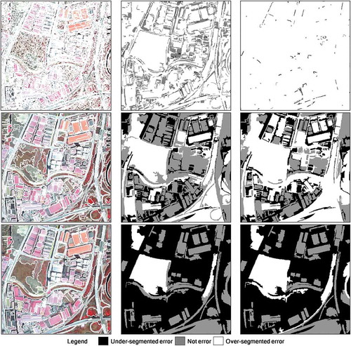
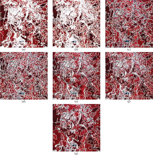
In addition to the analysis of γ, a direct comparison is performed for the new and the old UOA. These results can be seen in Figure 5. For fair comparison, δs of the two UOA methods are fixed at 0.5. For the improved UOA, γ is set at 0.5, because this value is tested to be sufficiently effective for avoiding over-estimating OSE. In Figure 5, segmentation results of scale 10, 50 and 100 are exhibited. A visual comparison of the two right columns indicates that the old UOA produces more white regions than the counterpart (the segments that have OSE are colored as white, as illustrated by the legend of Figure 5), especially when scale is 10. For scale 50, where most rooftops are well singled out, the original UOA obviously have more mistakes in marking OSE. For example, the two orange rectangular roofs at the right top part are completely segmented out, but the old UOA identifies them as containing OSE while the new method correctly determines the two segments as not having segmentation error. As for scale 100, still more segments are colored white by the original UOA than the improved version, but this problem is less apparent than the results of lower scales, primarily due to that the scale of 100 leads to less OSE.

Figure 5. Comparison between the old and the new UOA methods. From left to right, the first, second and third column correspond to segmentation results, new UOA evaluation results, old UOA evaluation results, respectively. From top to bottom, the first, second and third row correspond to segmentation results generated by using scale 10, 50 and 100, respectively.

From the above experimental descriptions, it can be concluded that the proposed UOA can avoid the issue of over-estimating OSE, but its performance is evidently affected by the parameter γ. Thus, it is necessary to test the effects of this threshold on the segmentation results of the proposed region merging approach.

3.3. Parameter analysis for the proposed region merging

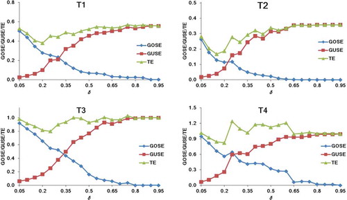
As delineated in section 2, there are totally four parameters for the proposed method: S (shape coefficient), C (compactness coefficient), δ and γ. The former two are associated with the heterogeneity change-based merging criterion, which has been extensively analyzed in a previous study (Schultz et al. 2015). Therefore, this work only focuses on the analysis of δ and γ. S, C are, respectively, fixed at 0.1, 0.5 throughout this work. In the experiment of this sub-section, a series of segmentation results are produced by using the proposed segmentation approach, parameterized by δ and γ both ranging from 0.05 to 0.95 with 0.05 as the incremental step, leading to 361 segmentation results for each test image.

To accurately reflect the segmentation quality of those results, the supervised evaluation method employed in the previous sub-section is adopted, resulting in the graphs in Figs. 6 and 7. Since GOSE/GUSE merely quantifies OSE/USE for all of the reference segments, and the two types of segmentation error are independent, it is not straightforward to use them to identify the optimal result from a series of segmentations. Thus, in this study a new score, named total error (TE), is devised:

(6) $\mathrm{T}\mathrm{E}=\mathrm{G}\mathrm{O}\mathrm{S}\mathrm{E}+\mathrm{G}\mathrm{U}\mathrm{S}\mathrm{E}$(6)

Figure 6. Results of parameter analysis. From top to bottom, the first, second and third rows show the quantitative evaluation results of GOSE, GUSE, and TE, respectively. The left and right columns correspond to T1 and T2, respectively.

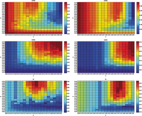
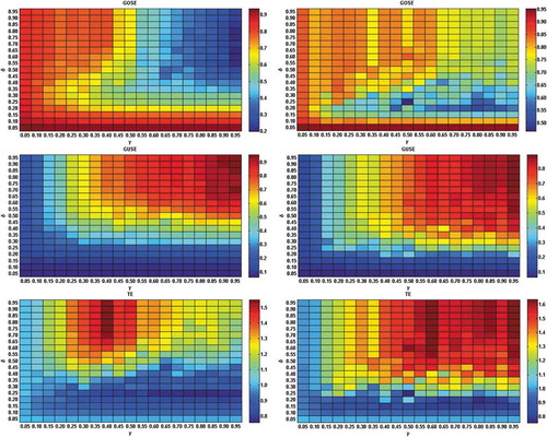
Figure 7. Results of parameter analysis. From top to bottom, the first, second and third rows show the quantitative evaluation results of GOSE, GUSE and TE, respectively. The left and right columns correspond to T3 and T4, respectively.

For a segmentation result, if either GOSE or GUSE is high, its TE will not be low, indicating low segmentation quality. Only if both GOSE and GUSE are small, the segmentation can be considered good. Thus, in theory, the best segmentation quality should correspond to the lowest TE.

Figs. 6 and 7 illustrate the GOSE, GUSE, and TE for all of the combinations of δ and γ for the four test images. By observing these graphs, it can be seen that the four images shared a similar trend that when δ is fixed, GOSE/GUSE generally decreases/increases. Moreover, the highest GOSE/GUSE occurs when both δ and γ have the smallest/largest value. The lowest TE corresponds to the combination of δ = 0.20, γ = 0.75 for T1, δ = 0.20, γ = 0.95 for T2, δ = 0.25, γ = 0.75 for T3, δ = 0.20, γ = 0.80 for T4. Those configurations are thus determined as optimal for the four test images.

According to Figure 6, it is interesting to see that for a relatively large scope, TE is obviously low and has small variance. Such a scope is delimited by δ∈[0.15, 0.25], γ∈[0.65, 0.95] for T1, and by δ∈[0.10,0.20], γ∈[0.70,0.95] for T2. These two scopes are similar in size and location in δ-γ plane, which may be attributed to the similar characteristics of T1 and T2. On the contrary, T3 and T4 have a different pattern. By observing Figure 7, it can be noticed that there is also a scope in which TE is low-valued for both T3 and T4. However, the low-TE δ-γ scopes of T3 and T4 are relatively smaller and less evident than those of T1 and T2.

Based on the aforementioned observation, it can be deduced that for urban or agricultural areas, δ is suggested to be set between 0.1 and 0.3, and δ is suggested to be set larger than 0.6. However, for images mostly covering natural geo-objects, parameter tuning is suggested, since the optimal setting may vary for different scenes. The experiment of T3 and T4 implies that the optimal setting for natural landscape images probably exists in the lower-right half of δ-γ plane, i.e., δ < 0.5 and γ > 0.5.

Since the aforementioned experiments are all completed by using the band combination of near-infrared, red and green channels, while there exist four spectral bands for the four images, it is necessary to investigate the effects of band combination on segmentation performance. Figure 8 is demonstrated for this purpose. Note that since the results of the four images have quite similar patterns, only the result of T1 is provided. For fair comparison, for each band combination, the average performance score is chosen to plot Figure 8. The average score is computed by using all of the δ-γ settings in the scope delimited by δ∈[0.15, 0.25], γ∈[0.65, 0.95]. In Figure 8, N, R, G, B in the abscissa represent the near-infrared, red, green and blue spectral band, respectively.

Figure 8. Effects of band combination on segmentation performance of T1. The left shows the variance of GOSE, GUSE, TE for different band combinations, while the right demonstrates the computational time.

It can be seen that the combination of NRG produced the lowest TE. Although the computational time of one- and two-band combinations is apparently lower than that of NRG, 4.5-s is acceptable. Using all of the four channels leads to the fourth lowest TE, but it has the longest computational time. Due to this analysis, NRG is adopted in the following experiments.

3.4. Comparative experiment

To validate the proposed segmentation technique, five state-of-the-art approaches are utilized for comparative study. They are introduced as follows.

1. Hybrid region merging (HRM) (Zhang et al. 2014). It is based on the well-known multi-resolution segmentation (MRS) (Baatz and Schäpe 2000). Its merging criterion is identical to that of MRS, and the two related coefficients, S and C, are, respectively, fixed as 0.1 and 0.5 in this experiment.

2. Hierarchical segmentation (HSEG) (Tilton et al. 2012). It exploits band means squared error as the merging criterion. HSEG can merge nonadjacent segments to enhance segmentation quality, but this significantly widens the searching space and accordingly aggravates the computational burden. Thus, this function is not initiated.

3. Scale-variable region merging (SVRM) (Yang, He, and Caspersen 2017). It can locally alter scale parameter (SP) according to the spectral heterogeneity of the segment being processed, so that differently sized geo-objects can be better singled out than the traditional scale-fixed strategy. The merging criterion is based on spectral angular mapping.

4. Size-constrained region merging with edge penalty (SCEP) (Chen, Qiu, and Wu 2015). It has two characteristics: first, it can avoid merging two segments having large difference in size; second, edge information is used in its merging criterion. The second characteristic is similar to the model proposed in this work (Equation (4)), but the metric of SCEP is based on exponential function, the computation of which relies on a parameter, e. By comparison, Equation (4) is parameter-free.

5. Region merging guided by priority (RMGP) (Su 2017b). Its main advantage resides in its merging sequence, which is controlled by inter- and intra-segment heterogeneity. The inter-segment heterogeneity is modeled by using edge information, but only the pixels situating at the common boundary of two segments are considered.

It is important to note that the most important parameter for the five approaches mentioned above is the scale parameter (SP). Therefore, for each method, a series of SPs are tested and the one with the smallest TE is chosen for comparison. The parameter configurations for the four test images are listed in Table 4.

Table 4. Optimal parameter settings for T1, T2, T3, and T4.

Method	T1						T2						T3						T4
	δ	γ		S		C	δ	γ		S		C	δ	γ		S		C	δ	γ		S		C
IUOAS	0.20	0.75		0.1		0.5	0.20	0.95		0.1		0.5	0.25	0.75		0.1		0.5	0.20	0.80		0.1		0.5
	δ		S		C		δ		S		C		δ		S		C		δ		S		C
OUOAS	0.20		0.1		0.5		0.15		0.1		0.5		0.25		0.1		0.5		0.20		0.1		0.5
	S		C		SP		S		C		SP		S		C		SP		S		C		SP
HRM	0.1		0.5		50		0.1		0.5		40		0.1		0.5		40		0.1		0.5		40
	SP						SP						SP						SP
HSEG	70						60						40						50
	SP						SP						SP						SP
SVRM	2.5						2.0						1.5						1.0
	t		e		SP		t		e		SP		t		e		SP		t		e		SP
SCEP	200		0.10		60		200		0.05		70		200		0.10		50		200		0.15		30
	α		γ		SP		α		γ		SP		α		γ		SP		α		γ		SP
RMGP	0.5		0.5		20		0.5		0.5		30		0.5		0.5		30		0.5		0.5		20

Aside from the five competitive techniques, a region merging integrated with the original UOA is implemented and used in this experiment. For convenience, the proposed method is termed as IUOAS (improved UOA segmentation), and the algorithm based on the original UOA is addressed as OUOAS (original UOA segmentation) in the following. Since the merging criterion of IUOAS and OUOAS is the same, the inclusion of OUOAS helps to unveil the effects of the improved UOA on segmentation performance. There are three parameters in OUOAS: S, C, and δ. The former two are identically set as those in IUOAS. As for δ, its optimal values for the test images are selected according to Figure 9. Note that the parameter setting for IUOAS is determined according to the experiment in sub-section 3.3.

Figure 9. GOSE, GUSE and TE curves of the OUOAS for the four test images. These graphs are used to determine the optimal δ values for OUOAS.

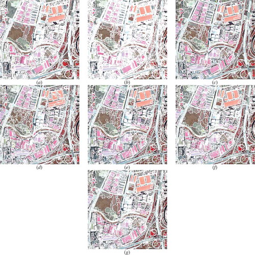
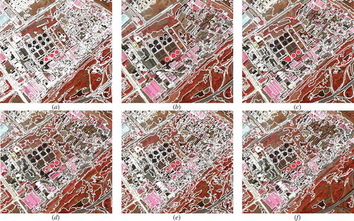
Visual comparison is initially used to assess the performance of the seven segmentation algorithms. The segmentation results for the four test images can be observed from Figures 10–13. For artificial-object-dominant scenes (T1 and T2), IUOAS and OUOAS well delineate the major geo-objects, although the latter produces OSE for many heterogeneous geo-objects, which is probably caused by its inferior ability to identify over-segmented segments. HRM and RMGP have competitive results, but the former yields more visually pleasing results than the latter for both T1 and T2. RMGP under-segments some aqua-cultural pools for T2, which are homogeneous. As for the other three methods, OSE can be evidently seen, since many buildings in T1 and water pools in T2 are fragmented in the results of the three approaches.

Figure 10. Segmentation results for T1. (a) IUOAS, (b) OUOAS, (c) HRM, (d) HSEG, (e) SVRM, (f) SCEP, (g) RMGP.

Compared to T1 and T2, it is more difficult to segment the natural-object-dominant scenes (T3 and T4). Because unlike artificial geo-objects, such as buildings, roads, and aqua-cultural pools, natural geo-objects have fuzzier inter-segment boundary and higher intra-segment heterogeneity. Thus, the results shown in Figures 12 and 13 are not visually superior to the counterparts in Figures 10 and 11. It can be seen from Figures 12 and 13 that IUOAS produces competitive segmentation results, although many snow caps in T3 and most wetlands in T4 are fragmented. OUOAS has much more serious OSE for T3 and T4, which proves that IUOAS benefits greatly from the improved UOA. For T3, HRM and HSEG have relatively high OSE for some large geo-objects. SVRM, SCEP, and RMGP perform better for extracting large objects in T3, but OSE still appears in snow cap area. For T4, HRM and SCEP generate comparatively good segmentation results, while HSEG results in serious OSE. RMGP and SVRM produce obvious USE.

Figure 11. Segmentation results for T2. (a) IUOAS, (b) OUOAS, (c) HRM, (d) HSEG, (e) SVRM, (f) SCEP, (g) RMGP.

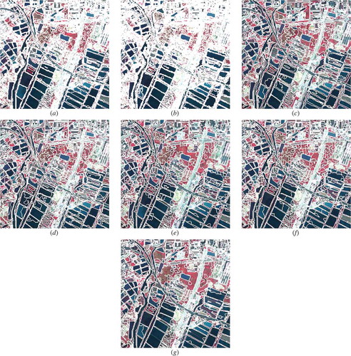
Figure 12. Segmentation results for T3. (a) IUOAS, (b) OUOAS, (c) HRM, (d) HSEG, (e) SVRM, (f) SCEP, (g) RMGP.

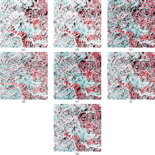
Figure 13. Segmentation results for T4. (a) IUOAS, (b) OUOAS, (c) HRM, (d) HSEG, (e) SVRM, (f) SCEP, (g) RMGP.

In addition to visual analysis, a quantitative evaluation is conducted by using GOSE, GUSE and TE metrics. Table 5 provides the evaluation scores for the four images. These scores agree well with the visual comparison. IUOAS and OUOAS consistently have the best and the second best TE score for the four images, respectively. HRM has the lowest GOSE value for T1, T3, and T4. SVRM yields the highest TE value for the four images. These results indicate that the proposed technique can produce competitive segmentation performance for high resolution remote sensing images.

Table 5. Quantitative evaluation scores for the optimal results derived by using the seven segmentation approaches. The best and the second best scores for each metric was highlighted in bold and italic, respectively.

Method	T1			T2			T3			T4
	GOSE	GUSE	TE	GOSE	GUSE	TE	GOSE	GUSE	TE	GOSE	GUSE	TE
IUOAS	0.2779	0.1012	0.3791	0.0856	0.0578	0.1434	0.5417	0.2184	0.7601	0.5006	0.2563	0.7569
OUOAS	0.2789	0.1014	0.3803	0.1278	0.0396	0.1674	0.5477	0.2516	0.7993	0.5621	0.2613	0.8234
HRM	0.1403	0.2501	0.3904	0.0781	0.1212	0.1993	0.3075	0.4961	0.8036	0.3230	0.4591	0.7891
HSEG	0.2134	0.1875	0.3999	0.1001	0.0946	0.1947	0.5425	0.2720	0.8145	0.4861	0.3863	0.8724
SVRM	0.2257	0.2168	0.4425	0.1022	0.1260	0.2282	0.4255	0.5571	0.9826	0.6055	0.7403	1.3458
SCEP	0.2317	0.1555	0.3872	0.0941	0.1073	0.2014	0.5132	0.2564	0.7696	0.4520	0.3482	0.8002
RMGP	0.2251	0.1581	0.3832	0.0525	0.1462	0.1987	0.5351	0.2493	0.7844	0.3617	0.5558	0.9175

3.5. Comparative experiment of a large image

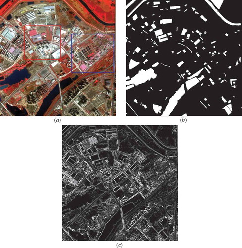
The aforementioned experimental results demonstrate the superiority of the proposed segmentation algorithm. However, the sizes of the four images are relatively small, and in many operational situations, the images to be processed are much larger. Therefore, another experiment is conducted by using a larger scene, which is a Gaofen-2 image subset of 1000 × 1000 pixels, as shown in Figure 14(a). This image is coded as T5. Various types of geo-objects exist in this scene, including buildings, shadows, roads, bare lands, vegetated areas, lakes, rivers, water ponds. They vary greatly in spectra and size, making it difficult for successful segmentation. Since T5 and T1 are extracted from the same GaoFen-2 image, the basic information of T5 can be found in Table 3. To enable supervised evaluation, 146 reference geo-objects are manually extracted by an expert, as shown in Figure 14(b). Its edge strength map is illustrated in Figure 14(c).

Figure 14. The large image (T5) used for the experiment in sub-section 3.5. (a) The false-color image (R: Near-infrared, G: Red, B: Green). (b) The reference geo-objects manually extracted by an expert. (c) The edge strength map.

Six methods are employed in this experiment: IUOAS, HRM, HSEG, SVRM, SCEP, and RMGP. The parameters of these methods are fine-tuned, meaning that for each algorithm, the result corresponding to the lowest TE is selected for comparison. The parameter settings for the six methods are listed in Table 6.

Table 6. Parameter setting for the six algorithms used in the experiment of T5.

Method	Parameter setting
	δ	γ	S	C
IUOAS	0.3	0.7	0.1	0.5
	S	C	SP
HRM	0.1	0.5	100
	SP
HSEG	150
	SP
SVRM	4.5
	t	e	SP
SCEP	200	0.1	100
	α	γ	SP
RMGP	0.5	0.5	50

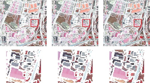
The segmentation results of the six techniques are shown in Figure 15. An initial observation reveals that HRM, HSEG, and SVRM have the most serious OSE for large geo-objects in T5, since the lakes located at the bottom-left part are over-segmented by these algorithms. IUOAS, SCEP, and RMGP extract more complete segments for these lakes. To analyze the segmentation results of urban areas in T5, the red and blue rectangles in Figure 14(a) are used, leading to the zoomed-in images shown in Figures 16 and 17.

Figure 15. Segmentation results of the six algorithms for T5. (a) IUOAS. (b) HRM. (c) HSEG. (d) SVRM. (e) SCEP. (f) RMGP.

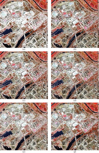
Figure 16. Subset segmentation results of the six methods for T5. This subset corresponds to the red rectangle in Figure 14(a). (a) IUOAS. (b) HRM. (c) HSEG. (d) SVRM. (e) SCEP. (f) RMGP.

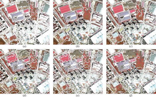
Figure 17. Subset segmentation results of the six methods for T5. This subset corresponds to the blue rectangle in Figure 14(a). (a) IUOAS. (b) HRM. (c) HSEG. (d) SVRM. (e) SCEP. (f) RMGP.

From Figure 16, it can be seen that IUOAS, HRM, and HSEG outperform the other three methods in delineating rooftops. Although the shadow areas in the middle part of this subset are better singled out by HSEG and SVRM, such an advantage is not very conspicuous. As for the bare soil regions, HRM yields the most visually pleasing performance, but IUOAS, HSEG, and RMGP also well reflect the structure of these geo-objects.

The results of Figure 17 are very interesting. IUOAS and SCEP out-perform the other methods in singling out the circular objects situated at the middle part of this subset, and the former is better than the latter in preserving the shapes of these small geo-objects. As for the lower-right part of this subset, HRM and HSEG have the most accurate segmentation, since roads and bare soils are well segmented out in their results. RMGP apparently under-segments this region. Although IUOAS well partitions the major geo-objects of this area, the trunk road is over-segmented, which is probably due to the new edge-based merging criterion.

Quantitative evaluation results listed in Table 7 have a relatively good agreement with the aforementioned analysis. It can be noticed that the proposed method is superior to the other five approaches in terms of GOSE, GUSE, and TE. HRM and HSEG perform equivalently, since their scores are very similar. Unexpectedly, SVRM produces the worst GOSE and TE. A possible reason is its spectral angle mapper-based merging criterion, which has a small numerical range (it is (0,π/2), while the counterparts of other methods are (0,+∞).), thus some inappropriate merging cannot be avoided. Another explanation is its relatively simple scale-variable strategy, which may not be effective for a complicated scene like T5. Table 7 also tabulates the running time of the six algorithms. It can be seen that the proposed technique is comparatively time-consuming, probably due to the repetitive computation of the improved UOA. All of the experiments in this study are conducted on a personal computer equipped with an Intel I5-6500 CPU @ 3.2 GHz, 8 GB memory, and 64-bit Windows 7 operating system, and all of the algorithms are written in C++.

Table 7. Performance scores and execution time of the six algorithms for the experiment of T5. The best score for each metric is highlighted in bold.

Method	GOSE	GUSE	TE	Time(s)
IUOAS	0.1626	0.1543	0.3169	102
HRM	0.2268	0.2783	0.5051	37
HSEG	0.2719	0.2292	0.5011	21
SVRM	0.3552	0.3706	0.7258	106
SCEP	0.2871	0.2930	0.5801	117
RMGP	0.1870	0.3997	0.5867	109

4. Discussion

Improving segmentation accuracy is the main objective of this study. To achieve this goal, two contributions are made: (1) an improved UOA evaluation metric, and fuse it with a region merging technique, (2) a new merging criterion by using edge information. The most innovative idea is represented by the first contribution, since previous studies rarely fused UOA with region merging. Tables 5 and 7 indicate that the TE scores of IUOAS are averagely 0.1139 lower than the counterparts of the other algorithms. It is thus necessary to discuss the advantage and limitation of the proposed technique.

Since IUOAS is based on region merging, the principle of this type of algorithm needs to be discussed before explaining the merit of IUOAS. In a region merging process, geo-objects are extracted by merging small segments. Such segments can be considered as having an over-segmentation error (OSE). By contrast, when a geo-object has been completely singled out as one segment, the merging of it should be avoided, because if it is merged, under-segmentation error (USE) will be created. How to reduce OSE and USE becomes the key to the success of a region merging-based segmentation. By fusing UOA with a region merging method, the segments with OSE or USE can be identified, which guides the merging process to decrease segmentation error. In this manner, how to accurately assign the type of segmentation error to a segment plays a crucial role. Based on the experimental results in sub-section 3.4, it can be seen that OUOAS produces more OSE than IUOAS, which proves the significance of the improved UOA. According to sub-section 2.2, the defect of the original UOA tends to miss-detect OSE, thus some appropriate merging cannot be executed, leading to serious OSE in the results of OUOAS, as can be observed in the corresponding sub-figures from Figures 10–13.

According to the obtained results shown in sub-sections 3.4 and 3.5, the methods used for comparison (HRM, HSEG, SVRM, SCEP, RMGP) have competitive segmentation accuracy. All of these methods, and many other state-of-the-art methodologies (Xiong et al. 2018; Liu, Du, and Mao 2017; Su 2017a; Zhou et al. 2017), rely on scale parameter (SP) to control the size of the resulted segments, thus it is easy to understand that SP directly affects segmentation quality for these approaches. On the contrary, for the proposed technique, there is no SP. Instead, two parameters (δ and γ) are used. Although these parameters serve similarly as SP, their influences on segmentation accuracy are not straightforward. This causes a limitation, that is, it is relatively difficult to select the optimal setting for δ and γ. The results are shown in Figures 6 and 7 support this statement.

Another drawback of IUOAS is that for heterogeneous areas, small segments are created, leading to obvious OSE. For example, in Figure 10(a), small segments dominate the built-up geo-objects and the periphery of roads. This may be resulted from the OSE miss-detection of the improved UOA for these small segments. A potential solution is to further merge the small segments after the process of IUOAS. To achieve this, a simple merging process called size-merge is added to IUOAS. Size-merge is initiated after the execution of IUOAS. In its process, a segment smaller than a threshold (T_size) is merged with its nearest neighbor, so that OSE can be reduced. To validate this approach, size-merge-added IUOAS is performed for T1, and the results of different T_size values are exhibited in Figure 18. By observing the zoomed-in areas in Figure 18, it can be seen that as T_size increases, small segments become fewer. However, quantitative evaluation for these results (listed in Table 8) indicates that although GOSE declines with the increase of T_size, TE rises, implying that the overall segmentation quality is negatively influenced by larger T_size. When T_size = 0, size-merge is not executed, but its TE ranks the first in Table 8. A possible explanation for this phenomenon is that size-merge is too simple to remarkably raise segmentation accuracy. Thus, more complicated techniques are needed, but this is beyond the scope of this article.

Table 8. Quantitative evaluation results of size-merge-added IUOAS.

Tsize	GOSE	GUSE	TE
0	0.2779	0.1012	0.3791
10	0.2666	0.1231	0.3897
30	0.2534	0.1400	0.3934
50	0.2401	0.1518	0.3919

Figure 18. Segmentation results of size-merge-added IUOAS. The top row shows the segmentation results, and the bottom row displays the zoomed-in area marked by the red rectangles. From left to right, the first, second, third column correspond to the results produced by using T_size = 10, 30, 50, respectively.

Based on the aforementioned discussions, it can be seen that the proposed approach still needs improvement. Further, improving UOA may help enhance the performance of the proposed IUOAS, and this may become our future research direction. Moreover, how to increase running efficiency for the proposed technique is also worth exploring, since the computational time reported in Table 7 is not advantageous for IUOAS.

5. Conclusion

This paper presents a new image segmentation algorithm. In order to improve segmentation accuracy, two major contributions are made. The most important contribution is an improved version of UOA, and it is fused with a region merging method. The other contribution includes a new edge-based merging criterion. Five scenes of remotely sensed images are utilized for experiment. To enable quantitative evaluation, three metrics including GOSE, GUSE, and TE are adopted. The proposed segmentation algorithm achieved TE values of 0.3791, 0.1434, 0.7601, 0.7569, and 0.3169 for T1, T2, T3, T4, and T5, respectively, which are consistently better than the other methods used for comparison. Since TE reflects overall segmentation performance, the experimental results indicate that the proposed segmentation method can produce superior segmentation quality.

Disclosure statement

No potential conflict of interest was reported by the author.

Additional information

Funding

This work is funded by the national natural science foundation of China, under grant number of 61701265. The anonymous reviewers are thanked for their constructive comments that helped improve this article.

References

- Adams, R., and L. Bischof. 1994. “Seeded Region Growing.” IEEE Transactions on Pattern Analysis and Machine Intelligence 16 (6): 641–647. doi:10.1109/34.295913.
- Baatz, M., and M. Schäpe. 2000. “Multiresolution Segmentation - an Optimization Approach for High Quality Multi-Scale Image Segmentation.” Angewandte Geographische Informations Verarbeitung XII: 12–23.
- Beaulieu, J., and M. Goldberg. 1989. “Hierarchy in Picture Segmentation: A Step-Wise Optimization Approach.” IEEE Transactions on Pattern Analysis and Machine Intelligence 11: 150–163. doi:10.1109/34.16711.
- Blaschke, T. 2010. “Object-Based Image Analysis for Remote Sensing.” ISPRS Journal of Photogrammetry and Remote Sensing 65: 2–16. doi:10.1016/j.isprsjprs.2009.06.004.
- Blaschke, T., G. J. Hay, M. Kelly, S. Lang, P. Hofmann, E. Addink, R. Q. Feitosa, et al. 2014. “Geographic Object-Based Image Analysis Towards a New Paradigm.” ISPRS Journal of Photogrammetry and Remote Sensing 87: 180–191. doi:10.1016/j.isprsjprs.2013.09.014.
- Böck, S., M. Immitzer, and C. Atzberger. 2017. “On the Objectivity of the Objective Function—Problems with Unsupervised Segmentation Evaluation Based on Global Score and a Possible Remedy.” Remote Sensing 9 (8): 1–9. doi:10.3390/rs9080769.
- Cai, J., B. Huang, and Y. Song. 2017. “Using Multi-Source Geospatial Big Data to Identify the Structure of Polycentric Cities.” Remote Sensing of Environment 202: 210–221. doi:10.1016/j.rse.2017.06.039.
- Castilla, G., G. J. Hay, and J. R. Ruiz. 2008. “Size-Constrained Region Merging (SCRM): An Automated Delineation Tool for Assisted Photo Interpretation.” Photogrammetry Engineering Remote Sensing 74 (4): 409–419. doi:10.14358/PERS.74.4.409.
- Chen, B., F. Qiu, and B. Wu. 2015. “Image Segmentation Based on Constrained Spectral Variance Difference and Edge Penalty.” Remote Sensing 7: 5980–6004. doi:10.3390/rs70505980.
- Chen, G., and Q. Weng. 2018. “Special Issue: Remote Sensing of Our Changing Landscapes with Geographic Object-Based Image Analysis (GEOBIA).” GIScience and Remote Sensing 55 (2): 155–158. doi:10.1080/15481603.2018.1436953.
- Chen, G., Q. Weng, G. I. Hay, and Y. He. 2018. “Geographic Object-Based Image Analysis (GEOBIA): Emerging Trends and Future Opportunities.” GIScience and Remote Sensing 55 (2): 159–182. doi:10.1080/15481603.2018.1426092.
- Chen, J., M. Deng, X. Mei, T. Chen, Q. Shao, and L. Hong. 2014. “Optimal Segmentation of a High-Resolution Remote-Sensing Image Guided by Area and Boundary.” International Journal of Remote Sensing 35 (19): 6914–6939. doi:10.1080/01431161.2014.960617.
- Costa, H., G. M. Foody, and D. S. Boyd. 2018. “Supervised Methods of Image Segmentation Accuracy Assessment in Land Cover Mapping.” Remote Sensing of Environment 205: 338–351. doi:10.1016/j.rse.2017.11.024.
- Devereux, B. J., G. S. Amable, and C. C. Posada. 2004. “An Efficient Image Segmentation Algorithm for Landscape Analysis.” International Journal of Applied Earth Observation and Geoinformation 6: 47–61. doi:10.1016/j.jag.2004.07.007.
- Finkel, R., and J. L. Bentley. 1974. “Quad Trees: A Data Structure for Retrieval on Composite Keys.” Acta Inform 4: 1–9. doi:10.1007/BF00288933.
- Fu, G., H. Zhao, C. Li, and L. Shi. 2013. “Segmentation for High-Resolution Optical Remote Sensing Imagery Using Improved Quad-Tree and Region Adjacency Graph Technique.” Remote Sensing 5: 3259–3279. doi:10.3390/rs5073259.
- Gofman, E. 2006. “Developing an Efficient Region Growing Engine for Image Segmentation.” In Proc. ICIP, 2413–2416. Atlanta, GA: IEEE.
- Grybas, H., L. Melendy, and R. G. Congalton. 2017. “A Comparison of Unsupervised Segmentation Parameter Optimization Approaches Using Moderate- and High-Resolution Imagery.” GISciences and Remote Sensing 54 (4): 515–533. doi:10.1080/15481603.2017.1287238.
- Guo, H. 2018. “Steps to the Digital Silk Road.” Nature 554 (2): 25–27. doi:10.1038/d41586-018-01303-y.
- Johnson, B., and Z. Xie. 2011. “Unsupervised Image Segmentation Evaluation and Refinement Using a Multi-Scale Approach.” ISPRS Journal of Photogrammetry and Remote Sensing 66: 473–483. doi:10.1016/j.isprsjprs.2011.02.006.
- Kim, H., and J. Yeom. 2014. “Effect of Red-Edge and Texture Features for Object-Based Paddy Rice Crop Classification Using RapidEye Multi-Spectral Satellite Image Data.” International Journal of Remote Sensing 35: 7046–7068.
- Lassalle, P., J. Inglada, J. Michel, M. Grizonnet, and J. Malik. 2015. “A Scalable Tile-Based Framework for Region-Merging Segmentation.” IEEE Transactions on Geoscience and Remote Sensing 53 (10): 5473–5485. doi:10.1109/TGRS.2015.2422848.
- Li, S., S. Dragicevic, F. A. Castro, M. Sester, S. Winter, A. Coltekin, C. Pettit, et al. 2016. “Geospatial Big Data Handling Theory and Methods: A Review and Research Challenges.” ISPRS Journal of Photogrammetry and Remote Sensing 115: 119–133. doi:10.1016/j.isprsjprs.2015.10.012.
- Liu, D., and F. Xia. 2010. “Assessing Object-Based Classification: Advantages and Limitations.” Remote Sensing Letters 1: 187–194. doi:10.1080/01431161003743173.
- Liu, J., M. Du, and Z. Mao. 2017. “Scale Computation on High Spatial Resolution Remotely Sensed Imagery Multi-Scale Segmentation.” International Journal of Remote Sensing 38 (18): 5186–5214.
- Liu, J., J. Li, W. Li, and J. Wu. 2016. “Rethinking Big Data: A Review on the Data Quality and Usage Issues.” ISPRS Journal of Photogrammetry and Remote Sensing 115: 134–142. doi:10.1016/j.isprsjprs.2015.11.006.
- Liu, J., H. Pu, S. Song, and M. Du. 2018. “An Adaptive Scale Estimating Method of Multi-Scale Image Segmentation Based on Vector Edge and Spectral Statistics Information.” International Journal of Remote Sensing 39 (20): 6826–6845. doi:10.1080/01431161.2018.1466077.
- Marpu, P. R., M. Neubert, H. Herold, and I. Niemeyer. 2010. “Enhanced Evaluation of Image Segmentation Results.” Journal of Spatial Science 55: 55–68. doi:10.1080/14498596.2010.487850.
- Qin, A. K., and D. A. Clausi. 2010. “Multivariate Image Segmentation Using Semantic Region Growing with Adaptive Edge Penalty.” IEEE Transactions on Image Processing 19: 2157–2170. doi:10.1109/TIP.2010.2045708.
- Salembier, P., and S. Foucher. 2016. “Optimum Graph Cuts for Pruning Binary Partition Trees of Polarimetric SAR Images.” IEEE Transactions on Geoscience and Remote Sensing 54 (9): 5493–5502. doi:10.1109/TGRS.2016.2566581.
- Schultz, B., M. Immitzer, A. R. Formaggio, I. D. A. Sanches, A. J. B. Luiz, and C. Atzberger. 2015. “Self-Guided Segmentation and Classification of Multi-Temporal Landsat 8 Images for Crop Type Mapping in Southeastern Brazil.” Remote Sensing 7: 14482–14508. doi:10.3390/rs71114482.
- Su, T. 2017a. “Efficient Paddy Field Mapping Using Landsat-8 Imagery and Object-Based Image Analysis Based on Advanced Fractal Net Evolution Approach.” GIScience and Remote Sensing 54 (3): 354–380. doi:10.1080/15481603.2016.1273438.
- Su, T. 2017b. “A Novel Region-Merging Approach Guided by Priority for High Resolution Image Segmentation.” Remote Sensing Letters 8 (8): 771–780. doi:10.1080/2150704X.2017.1320441.
- Su, T. 2018. “An Improved Unsupervised Image Segmentation Evaluation Approach Based on Under- and Over-Segmentation Aware.” ISPRS TC III Mid-term Symposium “Developments, Technologies and Applications in Remote Sensing”, Beijing, China. ISPRS Annals of the Photogrammetry, Remote Sensing and Spatial Information Sciences, IV-3 vols, 197–204. doi:10.3389/fncel.2018.00197.
- Su, T., and S. Zhang. 2017. “Local and Global Evaluation for Remote Sensing Image Segmentation.” ISPRS Journal of Photogrammetry and Remote Sensing 130: 256–276. doi:10.1016/j.isprsjprs.2017.06.003.
- Su, T., and S. Zhang. 2018. “Multi-Scale Segmentation Method Based on Hierarchical Merge Tree for High Resolution Imagery.” IEEE Access 6: 17801–17816. doi:10.1109/ACCESS.2018.2819988.
- Tilton, J. C., and E. Passoli. 2014. “Incorporating Edge Information into Best Merge Region-Growing Segmentation.” IGARSS 2014: 4891–4894. IEEE.
- Tilton, J. C., Y. Tarabalka, P. M. Montesano, and E. Gofman. 2012. “Best Merge Region-Growing Segmentation with Integrated Nonadjacent Region Object Aggregation.” IEEE Transactions on Geoscience and Remote Sensing 50 (11): 4454–4467. doi:10.1109/TGRS.2012.2190079.
- Troya-Galvis, A., P. Gançarski, N. Passat, and L. Berti-Équille. 2015. “Unsupervised Quantification of Under- and Over-Segmentation for Object-Based Remote Sensing Image Analysis.” IEEE Journal of Selected Topics in Applied Earth Observations and Remote Sensing 8 (5): 1936–1945. doi:10.1109/JSTARS.2015.2424457.
- Valero, S., P. Salembier, and J. Chanussot. 2013. “Hyperspectral Image Representation and Processing with Binary Partition Trees.” IEEE Transactions on Image Processing 22 (4): 1430–1443. doi:10.1109/TIP.2012.2231687.
- Vieira, M. A., A. R. Formaggio, C. D. Rennó, C. Atzberger, D. A. Aguiar, and M. P. Mello. 2012. “Object Based Image Analysis and Data Mining applied to a remotely sensed Landsat time-series to map sugarcane over large areas.” Remote Sensing of Environment 123: 1256–1265. doi:10.1016/j.rse.2012.04.011.
- Wu, A., T. Hong, and A. Rosenfeld. 1982. “Threshold Selection Using Quadtrees.” IEEE Transactions on Pattern Analysis and Machine Intelligence 4 (1): 90–94. doi:10.1109/TPAMI.1982.4767203.
- Xiong, Z., X. Zhang, X. Wang, and J. Yuan. 2018. “Self-Adaptive Segmentation of Satellite Images Based on a Weighted Aggregation Approach.” GISciences and Remote Sensing. doi:10.1080/15481603.2018.1504413.
- Yang, J., Y. He, and J. Caspersen. 2017. “Region Merging Using Local Spectral Angle Thresholds: A More Accurate Method for Hybrid Segmentation of Remote Sensing Images.” Remote Sensing of Environment 190: 137–148. doi:10.1016/j.rse.2016.12.011.
- Yang, J., Y. He, and Q. Weng. 2015. “An Automated Method to Parameterize Segmentation Scale by Enhancing Intrasegment Homogeneity and Intersegment Heterogeneity.” IEEE Geoscience and Remote Sensing Letters 12: 1282–1286. doi:10.1109/LGRS.2015.2393255.
- Yang, J., P. Li, and Y. He. 2014. “A Multi-Band Approach to Unsupervised Scale Parameter Selection for Multi-Scale Image Segmentation.” ISPRS Journal of Photogrammetry and Remote Sensing 94: 13–24. doi:10.1016/j.isprsjprs.2014.04.008.
- Yu, H., X. Zhang, S. Wang, and B. Hou. 2013. “Context-Based Hierarchical Unequal Merging for SAR Image Segmentation.” IEEE Transactions on Geoscience and Remote Sensing 51 (2): 995–1009. doi:10.1109/TGRS.2012.2203604.
- Yu, Q., and D. A. Clausi. 2008. “IRGS: Image Segmentation Using Edge Penalties and Region Growing.” IEEE Transactions on Pattern Analysis and Machine Intelligence 30: 2126–2139. doi:10.1109/TPAMI.2008.15.
- Yu, W., W. Zhou, Y. Qian, and J. Yan. 2016. “A New Approach for Land Cover Classification and Change Analysis: Integrating Backdating and an Object-Based Method.” Remote Sensing of Environment 177: 37–47. doi:10.1016/j.rse.2016.02.030.
- Zhang, X., P. Xiao, X. Feng, J. Wang, and Z. Wang. 2014. “Hybrid Region Merging Method for Segmentation of High-Resolution Remote Sensing Images.” ISPRS Journal of Photogrammetry and Remote Sensing 98: 19–28. doi:10.1016/j.isprsjprs.2014.09.011.
- Zhang, X., P. Xiao, X. Song, and J. She. 2013. “Boundary-Constrained Multi-Scale Segmentation Method for Remote Sensing Images.” ISPRS Journal of Photogrammetry and Remote Sensing 79: 15–25. doi:10.1016/j.isprsjprs.2013.01.002.
- Zhou, Y., J. Li, L. Feng, X. Zhang, and X. Hu. 2017. “Adaptive Scale Selection for Multiscale Segmentation of Satellite Images.” IEEE Journal of Selected Topics in Applied Earth Observations and Remote Sensing 10 (8): 3641–3651. doi:10.1109/JSTARS.2017.2693993.