Spatial variations of small phytoplankton contributions in the Northern Bering Sea and the Southern Chukchi Sea

Abstract

Phytoplankton size classes (hereafter, PSCs) were derived from satellite ocean color data using a present phytoplankton abundance-based optical algorithm in the northern Bering and southern Chukchi Seas to characterize the spatial and seasonal variations of the different PSC and investigate the contributions of small phytoplankton to the total phytoplankton biomass. The comparison results showed that the phytoplankton abundance-based method approach could reasonably classify the three PSCs (pico-, nano-, and micro phytoplankton). The satellite maps of the dominant PSCs were derived using long-term satellite ocean color data. The general spatial distribution showed that the large (micro-) phytoplankton were dominant in the coastal waters and the west side of the Bering strait, while the small size (nano- or pico-) phytoplankton were dominant in the open ocean waters. Nano- and microphytoplankton were dominant in May and October in most of the study area, while pico-phytoplankton were dominant in the summer months in the open ocean waters. The annual variation in small phytoplankton dominance had a strong positive relationship with the annual mean sea surface temperature (SST), which is consistent with the increasing dominance of small phytoplankton biomass as water temperature increases. Microphytoplankton have an apparent increasing trend in the southeastern Chukchi Sea but slightly decreasing trends in Chirikov and St. Lawrence Island Polynya (SLIP). In contrast, there were increasing trends in picophytoplankton in Chirikov and SLIP, which seems to be related to increasing annual SST. It is crucial to monitor changes in dominant groups of phytoplankton community in the Bering and Chukchi Seas as important biological hotspots responding to the recent changes in environmental conditions.

Keywords:

• phytoplankton size class
• chlorophyll-a
• ocean color remote sensing
• OC–CCI
• Bering sea
• Chukchi sea

1. Introduction

The Bering and Chukchi Seas are an important gateway connecting between the Pacific Ocean and the Arctic Ocean (Sambrotto, Goering, and McRoy 1984; Springer et al. 1993). The high-nutrient Pacific waters along the western side of the Bering and Chukchi Seas support a high primary production of phytoplankton, which subsequently sustain high biomasses of fishes, marine mammals, and seabirds as well as benthic communities (Springer et al. 1987; Grebmeier and McRoy 1989; Springer and McRoy 1993; Bluhm and Gradinger 2008; Grebmeier et al. 2015). Recent studies have reported that field-measured primary production rates are substantially lower than those previously reported from the northern Bering Sea and the Chukchi Sea several decades ago (Lee, Whitledge, and Kang 2007; Lee et al. 2012; Yun et al. 2016), although satellite-derived primary production has increased in the Chukchi Sea shelf (Arrigo, van Dijken, and Pabi 2008). In the Chukchi Sea, primary production is mainly controlled by major inorganic nutrient availability, which is strongly related to the freshwater content (Yun et al. 2016). Recently, several climate-induced environmental changes, such as a reduced maximum extent and the earlier melting of seasonal pack ice over the previous decades have been reported in the northern Bering Sea and the Chukchi Sea (Overland and Stabeno 2004; Grebmeier et al. 2006a; Bluhm and Gradinger 2008; Grebmeier et al. 2015). In addition, an increased volume flux (50%) accompanied by increases in heat and freshwater fluxes was reported in the Bering Strait throughflow (Woodgate, Weingartner, and Lindsay 2012). The recent increases in freshwater fluxes in the region could be substantial for primary production of phytoplankton because of potentially lower nutrient availability (Yun et al. 2016). Subsequent changes in higher trophic levels are anticipated in the northern Bering and Chukchi Seas directly linked to the marine ecosystems in the Arctic Ocean (Grebmeier 2012).

Phytoplankton as a basic primary producer can be a good indicator for marine ecosystem changes responding to environmental changes (Falkowski and Raven 1997; Yoder and Kennelly 2003; Moline et al. 2004; Wassmann et al. 2011; Lee et al. 2017). For example, the contributions of small phytoplankton to the total biomass and production of the phytoplankton community could be increased and became more important under warming ocean conditions (Morán et al. 2010; Li et al. 2009; Lee et al. 2013). In the Canada Basin, Li et al. (2009) found that stronger stratification and consequently lower nutrient conditions in the upper water column caused by recent warming and freshening surface waters resulted in a shift into thriving pico-size phytoplankton from larger cells. Therefore, it is important to know what extent the smaller fraction of the phytoplankton contributes to the overall biomass in marine ecosystems because of their potential impacts on total primary production under further ongoing environmental changes (Lee et al. 2013).

Satellite remote sensing data can provide a synoptic view of the optical properties in the upper waters from basin to global scale oceans with high temporal and spatial resolution (Son et al. 2005, 2014; Kim et al. 2018). Various algorithms to derive phytoplankton functional types (PFT) or phytoplankton size classes (PSCs) have been developed for satellite ocean color remote sensing data (Sathyendranath et al. 2004; Alvain et al. 2005; Devred. et al. 2006; Uitz et al. 2006; Hirata et al. 2008; Kostadinov, Siegel, and Maritorena 2010; Brewin et al. 2011). The PSC algorithms generally produce the most common phytoplankton groups, such as pico-, nano-, and microplankton. A phytoplankton abundance-based approach is commonly used for PSC algorithms. The abundance-based method relies on the relationship between PSCs and biogeochemical parameters such as Chl-a or the bio-optical properties of phytoplankton (Sathyendranath et al. 2004; Devred. et al. 2006; Uitz et al. 2006; Hirata et al. 2008). Satellite-derived phytoplankton classes provide effective insights to investigate the spatial and temporal patterns of phytoplankton communities and the dynamics of the marine food webs and to further understand the roles of phytoplankton communities in the global carbon cycles and climate changes (Bracher et al. 2017).

Our main objectives in this study are to derive the dominant phytoplankton size classes (PSCs) from satellite ocean color data, characterize the seasonal and interannual variations in the different cell-sized compositions of phytoplankton, and determine the contributions of small phytoplankton to the total chlorophyll-a concentrations using the long-term satellite ocean color data in the northern Bering and Chukchi Seas from 1998 to 2016.

2. Materials and methods

2.1. Study area

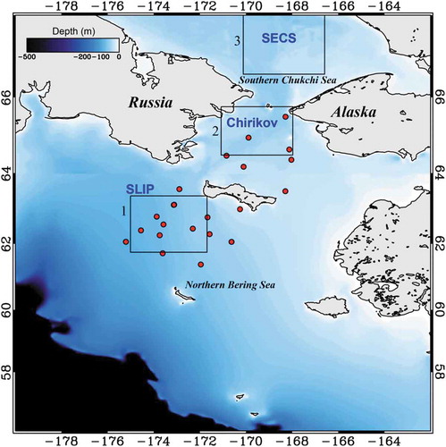
The international distributed biological observatory (DBO) program in the Pacific Arctic region was developed to monitor seasonally and annually the ecosystem response to climate-induced environmental changes such as recent pacific Arctic sea ice retreats (Grebmeier et al. 2010, 2015). Four regions in the northern Bering and Chukchi Seas, the St. Lawrence Island Polynya (SLIP; 61.75–63.37°N, 171.69–175.01°W), the Chirikov Basin (Chirikov; 64.49–65.76°N, 167.97–171.08°W), the Southeastern Chukchi Sea (SECS; 66.58–68.59°N, 166.59–173.12°W), and the Northeastern Chukchi Sea (NECS; 70.62–72.37°N, 158.46–165.46°W), were selected for an international network of research ship operations to coordinate seasonal and annual observations (Grebmeier et al. 2010). This DBO program helps evaluate ecosystem status in these four regions, which are areas of high biological productivity (Grebmeier et al. 2015). In this study, we focused on the three subregions, SECS, Chirikov, and SLIP, as shown in Figure 1, based on the field measurements obtained from the Chirikov and SLIP.

Figure 1. Map of the Northeastern Bering Sea and south Chukchi Sea with locations of in situ measurements during the Healy 2007 Cruise (May 14–18 June 2007). Filled circles are the observation stations for the cell-sized phytoplankton chlorophyll-a concentrations and optical measurements in May and June of 2007, and “x” symbols indicate stations NWC2 (st. 109) and ANSC (st. 51). Boxes indicate three subregions: (1) St. Lawrence Island Polynya (SLIP): 61.75°N – 63.37°N and 171.69°W – 175.01°W, (2) Chirikov Basin (Chirikov): 64.49°N – 65.76°N and 167.97°W – 171.08°W, and (3) Southeastern Chukchi Sea (SECS): 66.58°N – 68.59°N and 166.59°W – 173.12°W.

2.2. In-situ chlorophyll-a and optical measurements

Water samples (approximately 600 mL) for size-fractionated (0.7, 5, and 20 μm for the pico-, nano-, and microphytoplankton, respectively) chlorophyll-a (Chl-a) concentrations were obtained from six light depths (100%, 50%, 30%, 12%, 5%, and 1% penetration of the surface photosynthetically active radiation, PAR) at 23 productivity stations in the northern Bering Sea onboard the USCGC Healy from May 18 to 18 June 2007 (Figure 1). Twenty-three water samples taken at the surface were used for this study. Only two of the stations (NWC2 and ANSC) had sea ice cover (30 ~ 90%) (Lee et al. 2012). The six light depths were determined from an underwater PAR sensor (QSP2300, Biospherical Instruments Inc.) lowered with a conductivity-temperature-depth (CTD) rosette sampler (Lee et al. 2012). The Chl-a concentrations were measured by a precalibrated fluorometer (10-AU, Turner Designs, US); after filters were extracted in 10 ml of 90% acetone for 24 h, the Chl-a concentrations were calculated based on the Chl-a method from Parsons, Maita, and Lalli (1984).

A high-resolution profiling reflectance and radiometer (PRR; Biospherical Instruments Inc., USA) was used for the optical measurements in the water column. The underwater profiler PRR800 and the surface unit PRR810 (PRR–800/810) simultaneously collected vertical profiles of the upwelling radiance (L_u(λ,z)) and the downwelling surface irradiance (E_s(λ,0⁺)) at 17 multispectral (ultraviolet to infrared red) wavelengths, including 13 visible (412, 443, 490, 510, 520, 532, 555, 565, 589, 625, 665, 683, and 710 nm) bands. More detailed information of the optical measurements can be found in Lee et al. (2018).

2.3. Satellite data

The European Space Agency (ESA) Ocean Colour Climate Change Initiative (OC-CCI) project generated the OC-CCI products that merged ocean color data from multiple ocean color sensors; the Sea-viewing Wide Field-of-view Sensor (SeaWiFS), the MODerate resolution Imaging Spectroradiometer (MODIS) on Aqua, the Medium Resolution Imaging Spectrometer (MERIS) on Envisat-1, and the Visible Infrared Imaging Radiometer Suite (VIIRS) on the Suomi National Polar-orbiting Partnership (SNPP) (Melin et al. 2017). The main objective of OC-CCI is to create a consistent, error-characterized time-series of ocean color products focusing on climate change studies (Brewin et al. 2015). The OC-CCI version 3.1 global Level-3 monthly ocean color products at 4 km resolution, such as the remote sensing reflectance (R_rs) and the inherent optical properties (IOP), from January 1998 to December 2016 were obtained from the ESA OC–CCI website (http://www.esa-oceancolour-cci.org/).

Sea surface temperature (SST) data from the Advanced Very High Resolution Radiometer (AVHRR), MODIS-Aqua, VIIRS provided by the Physical Oceanography Distributed Active Archive Center (PODAAC) at NASA Jet Propulsion Laboratory (https://podaac.jpl.nasa.gov/) and the Ocean Biology Processing Group (OBPG) at NASA Goddard Space Flight Center (https://oceandata.sci.gsfc.nasa.gov/), were used for this study. We obtained the AVHRR, MODIS-Aqua, and VIIRS monthly composite data at 4-km spatial resolution from May 1998 to December 2003, from July 2002 to December 2013, and from January 2012 to December 2016, respectively. The SST data in overlapped period between the different sensors were compared and averaged to ensure the consistency of the SST values obtained from several sensors. To determine the spatial variation, the SST were averaged in the domain of the three sub-regions, SECS, Chirikov, and SLIP.

2.3. Optical model for phytoplankton size classes

One abundance-based algorithm for the PSCs (Hirata et al. 2008) was used to derive the PSCs from the satellite ocean color data. Hirata’s threshold-based method (Hirata et al. 2008) uses a single variable, the absorption coefficient by phytoplankton at wavelength 443 nm, a_ph(443), or Chl-a, to quantify the dominant phytoplankton size classes as follows: a_ph(443) < 0.023 m⁻¹ for picoplankton; 0.023 ≤ a_ph(443) < 0.069 m⁻¹ for nanoplankton; 0.069 ≤ a_ph(443) m⁻¹ for microplankton. This algorithm was used to derive the PSC with the abundance-based algorithm (Hirata et al. 2008) for both the in situ measurements and the satellite ocean color data. The a_ph(443) data were derived from the in situ R_rs(λ) measurements using the commonly used semianalytical method for the IOP data, the quasi-analytic algorithm (QAA) version 5 (Lee, Carder, and Arnone 2002). The IOP product (a_ph(443)) from the OC-CCI data were also generated using QAA (Lee, Carder, and Arnone 2002).

3. Results and discussion

3.1. Comparison of field-measured and satellite-derived phytoplankton size classes

Table 1 summaries the Chl-a concentrations and the percentage of Chl-a from each size phytoplankton groups (pico-, nano-, and microphytoplankton). The dominant phytoplankton size groups were also generated from the in situ Chl-a measurements from the different phytoplankton size groups and the optical model-derived absorption coefficients for phytoplankton (a_ph(443)) for the 23 stations in the northern Bering Sea. The model-derived dominant phytoplankton groups were considerably well matched to those from the Chl-a measurements (about 70% of 23 stations), while there were no good matches at seven stations of the 23 stations. These stations had a strong sub-chlorophyll a maximum layer at the depths of 30–40 m during the cruise period in 2007 (Lee et al. 2013). Microphytoplankton were dominant at the 7 stations based on the field measurements but picophytoplankton were dominant based on the optics-derived phytoplankton functional types. Overall, our results indicate that the model-derived approach could reasonably classify the three different cell-sized phytoplankton classes with an accuracy of approximately 70% (Table 1).

Table 1. Chl-a concentrations and percentage of Chl-a from three difference phytoplankton size classes (pico, nano, and micro phytoplankton), and the dominant phytoplankton size classes from the in situ Chl-a measurements and the optical model.

St.	Field Measurements							PFT model
	Chl-a Concentration (mg/m^3)			Percentage (%)			Dominant Size Class	Dominant Size Class
	Micro (>20 μm)	Nano (5–20 μm)	Pico (<5 μm)	Micro	Nano	Pico
1	0.8589	0.0580	0.0830	85.9	5.8	8.3	M	M
6	0.8315	0.1058	0.0628	83.1	10.6	6.3	M	M
9	0.6005	0.2627	0.1368	60.1	26.3	13.7	M	M
14	0.8925	0.0474	0.0601	89.3	4.7	6.0	M	P
18	0.7996	0.0873	0.1131	80.0	8.7	11.3	M	N
22	0.5132	0.1290	0.3578	51.3	12.9	35.8	M	P
27	0.5106	0.1702	0.3191	51.1	17.0	31.9	M	P
31	0.8720	0.0449	0.0831	87.2	4.5	8.3	M	M
35	0.8669	0.0413	0.0918	86.7	4.1	9.2	M	M
41	0.9345	0.0335	0.0321	93.4	3.3	3.2	M	M
51	0.6400	0.1920	0.1680	64.0	19.2	16.8	M	P
57	0.7032	0.0134	0.2833	70.3	1.3	28.3	M	M
61	0.7535	0.0892	0.1573	75.3	8.9	15.7	M	P
65	0.9171	0.0534	0.0295	91.7	5.3	3.0	M	M
69	0.8633	0.0581	0.0786	86.3	5.8	7.9	M	M
73	0.9556	0.0265	0.0179	95.6	2.7	1.8	M	M
81	0.2875	0.1625	0.5500	28.8	16.3	55.0	P	P
103	0.9228	0.0329	0.0443	92.3	3.3	4.4	M	P
109	0.2646	0.1340	0.6014	26.5	13.4	60.1	P	P
115	0.4000	0.2000	0.4000	40.0	20.0	40.0	P	P
119	0.4018	0.1339	0.4643	40.2	13.4	46.4	P	P
137	0.2985	0.1493	0.5522	29.9	14.9	55.2	P	P
140	0.4065	0.1057	0.4878	40.7	10.6	48.8	P	P

3.2. Seasonal patterns of different phytoplankton size classes

Synoptic seasonal maps of PSC are derived using satellite ocean color data in the Bering and Chukchi Seas (Figure 2). Figure 2 provides the climatological (January 1998 to December 2016) monthly images of the different PSCs (pico-, nano-, and microphytoplankton) from May to October in the northern Bering and Chukchi Seas derived from the OC-CCI ocean color products. Since the Bering and Chukchi Seas are covered by ice and/or clouds due to the severe weather conditions from late fall to early spring, the ocean color of the satellite data was used only for the 6 months from May to October.

Figure 2. Climatology (1998 to 2016) monthly composite images of the OC–CCI–derived dominant phytoplankton size classes in (a) May, (b) June, (c) July, (d) August, (e) September, and (f) October (blue, green, and red colors indicate pico, nano, and micro phytoplankton dominant).

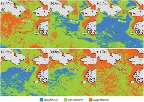
The overall spatial distribution of the PSCs images shows that large size (micro-) phytoplankton are dominant in the shallow (near/along coastal) waters and the west side of the Bering strait, while the small size (nano- or pico-) phytoplankton were dominant in the open ocean waters. In May, nanophytoplankton or microplankton were dominant in most of the study area (microphytoplankton in the northwestern Bering Sea and Alaskan coastal waters). In June, nano- and picophytoplankton were dominant in most of the northern Bering Sea. Picophytoplankton were particularly dominant in the open ocean waters of the Bering Sea (the southeastern area of the Gulf of Anadyr), while microphytoplankton were still dominant along the Alaskan coasts. In July, most of the northern Bering Sea was dominated by picophytoplankton, except the coastal waters. Nano- and microphytoplankton were dominant along the Alaskan coastal waters and the Bering strait. In August and September, the picophytoplankton-dominant area decreased in the northern Bering Sea, while nano- and microphytoplankton-dominant areas increased. Most of the coastal waters and the western Bering sea were dominated by microphytoplankton, and the middle of the northern Bering sea was dominated with nanophytoplankton in October.

In the SECS, the picophytoplankton increased from May (5.7%) to July (45.8%) and then decreased to September (5.6%) and October (7.4%). The nanophytoplankton decreased from May (65.4%) to July (44.9%) and then increased back to 63.8% in August and decreased in October (36.8%). The microphytoplankton decreased from May (28.9%) to July (9.3%) and then increased up to 55.8% in October. In Chirikov, the picophytoplankton increased from May (5.2%) to July (31.8%) and then showed no steady decrease trend, whereas the nanophytoplankton steadily increased from May (46.0%) to September (56.3%) and then decreased in October (46.8%). Microphytoplankton were dominant in most of the area in May (48.8%) and were lowest in July (19.1%) and then increased to approximately 35% until October. In SLIP, the picophytoplankton–dominant area increased from May (11.4% of the whole ocean in the study area) to July (92.3%) and then decreased to October (36.3%). In comparison, the contributions of nano- and microphytoplankton–dominant area were opposite to those of picophytoplankton. The contributions of nano- and microphytoplankton decreased from May to July and then increased in October. The monthly spatial distributions from May to October of the different PSCs (pico-, nano-, and microphytoplankton), especially for the picophytoplankton, matched well with the seasonal variation in the primary productivity of phytoplankton in the northern Bering and Chukchi Seas (Lee et al. 2012; Grebmeier et al. 2015). The primary productivity was generally high in May and June (the bloom period) and low throughout the summer season (July–September; the postbloom period) in the regions (Lee et al. 2012; Grebmeier et al. 2015). Normally, picophytoplankton are abundant in oligotrophic water conditions since they have an advantage for acquiring nutrients in low-nutrient waters (Agawin et al. 2000). Therefore, it appears reasonable to have a low contribution of picophytoplankton during the bloom period in May and June and a high contribution of picophytoplankton after the bloom period from July to September and vice versa for microphytoplankton (Figure 2).

3.3. Interannual variations of different phytoplankton size classes

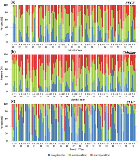
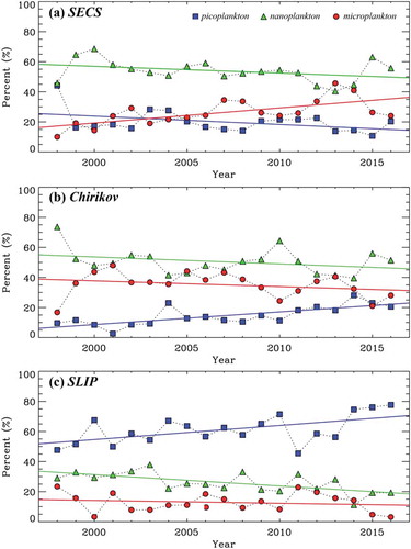
The long-term patterns of the three different PSCs in the three regions from 1998 to 2016 were investigated (Figure 3). Figure 3(a–c) shows the percentage of the dominant areas by each PSCs in the three subregions, the SECS, Chirikov, and SLIP, respectively. Because most of the study area was covered by ice and/or clouds, the satellite data were used only for the 6 months from May to October. In the SECS, the annual contributions of pico-, nano-, and microphytoplankton were 10.7–44.2%, 40.5–68.6%, and 10.0–45.7%, respectively. Overall, the dominant group in the SECS was nanophytoplankton (54.4% ± 7.8%), followed by microphytoplankton (26.1% ± 8.7%) and picophytoplankton (19.5% ± 7.2%). In Chirikov, the annual contributions of picophytoplankton and nanophytoplankton were 2.2–29.9% and 37.8–73.6%, respectively, whereas the contribution of microphytoplankton was 16.8% to 47.8%. The dominant phytoplankton in Chirikov were nanophytoplankton (49.0% ± 9.6%) followed by microphytoplankton (34.9% ± 8.0%) and picophytoplankton (16.1% ± 7.3%). In SLIP, the annual contributions of pico- and nanophytoplankton were 31.9–64.3% and 14.5–44.5%, respectively. In comparison, microphytoplankton contributed 4.8–44.1% to the total Chl-a compositions in SLIP. Overall, the dominant phytoplankton in SLIP were picophytoplankton (50.2% ± 8.6%) followed by nanophytoplankton (28.3% ± 8.0%) and microphytoplankton (21.5% ± 9.3%).

Figure 3. Monthly time series of percentages of the area dominated by pico (blue), nano (green), and micro (red) phytoplankton from the OC–CCI data in the three sub-regions, (a) SECS, (b) Chirikov, and (c) SLIP.

3.4. Comparison between sea surface temperature and small phytoplankton

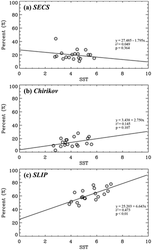
For comparison, our three groups of different cell-sized phytoplankton were classified into two groups: small (<5 µm; pico-) and large (>5 µm; nano- and micro-) phytoplankton. The annual averages of the satellite-derived SST from 1998 to 2016 were compared with the annual percentages of small picophytoplankton-dominant areas in the three subregions (Figure 4) to find the response of small phytoplankton to SST as an indicator of ongoing warming conditions (Li et al. 2009; Morán et al. 2010; Lee et al. 2013). The annual averages were calculated using the monthly SST and PSCs composite data of 6 months (May to October). A strong positive relationship was found between annual SST and annual small phytoplankton composition in the SLIP region (Figure 4(c); y = 6.643x + 25.203, r² = 0.4731, p < 0.01), which indicates that the annual variation in small phytoplankton dominance is strongly related with annual SST. This is consistent with the increasing dominance of small phytoplankton biomass as water temperature increases (Morán et al. 2010). In contrast, no strong relationships were found in the Chirikov and SECS regions (Figure 3(a,b)), which indicates that other environmental factors (e.g., currents and nutrients, as discussed below) rather than SST are more important for controlling the dominance of small phytoplankton biomass in these regions. The different physical environmental conditions were characterized among the SLIP, Chirikov, and SECS (Grebmeier et al. 2015). A strong northward advection of the nutrient-rich Anadyr water, fresh Alaska Coastal water, and intermediate-propertied Bering Sea water strongly influences the Chirikov and SECS regions, whereas relatively weaker, less variable flow conditions sustain the cold salty waters resulting from the sea ice production in the SLIP region compared to that occurring in the Chirikov and SECS regions (Grebmeier et al. 2015). The ratio of the three water masses varies seasonally and interannually (Coachman, Aagaard, and Tripp 1975), which strongly influences the physical conditions, nutrient dynamics, and consequently phytoplankton community, such as different cell size compositions and photosynthetic activities (Springer and McRoy 1993; Lee, Whitledge, and Kang 2007). In fact, Lee, Whitledge, and Kang (2007) found the two distinct size groups of phytoplankton community depending on the different water masses in the Bering Strait and the Chukchi Sea. Therefore, different PSC dominance in the Chirikov and SECS regions could be influenced largely by the dynamics of the northward three water masses rather than SST.

Figure 4. Annual mean (May to October) percentages of small (pico) phytoplankton-dominant areas from the OC–CCI data are compared with the satellite-derived annual mean SST (ºC) from 1998 to 2016 in (a) SECS, (b) Chirikov, and (c) SLIP.

3.5. Long-term trends of the three different PSC

The annual patterns of the three different PSCs and the SST in the northern Bering Sea and the southern Chukchi Sea from 1998 to 2016 are shown in Figure 5. The annual averages were calculated using the monthly composites of the satellite-derived PSCs and the SST data from 6 months (May to October). Pico- and nanophytoplankton were generally the dominant groups in the northern Bering Sea, whereas the predominant group was microphytoplankton in the Bering Strait, especially the western part. In comparison, nano- and microphytoplankton were the major groups occupying the southern Chukchi Sea during the observation period from 1998 to 2016. The annual SST patterns were similar in all three regions, showing strong interannual variations and slightly increasing trends.

Figure 5. Annual mean percentages of phytoplankton size classes, pico (blue), nano (green), and micro (red) phytoplankton, and SST in (a) SECS, (b) Chirikov, and (c) SLIP. The long-term trends (linear regressions) of the annual phytoplankton size classes and SST are derived as follows: (a) Pico: y = 1136.6–0.556x, r² = 0.178; Nano: y = 957.1–0.450x, r² = 0.124; Micro: y = – 1993.6 + 1.006x, r² = 0.430; SST: y = – 132.2 + 0.07x, r² = 0.176 in SECS, (b) Pico: y = – 1676.8 + 0.843x, r² = 0.547; Nano: y = 976.6–0.462x (r² = 0.097); Micro: y = 799.6–0.381x, r² = 0.070; SST: y = – 94.0 + 0.05x, r² = 0.096 in Chirikov, (c) Pico: y = – 1824.4 + 0.940x, r² = 0.305; Nano: y = 1535.7–0.752x, r² = 0.410; micro: y = 388.8–0.187x, r² = 0.029; SST: y = – 141.3 + 0.07x, r² = 0.173 in SLIP.

For the three DBO regions, picophytoplankton were generally the dominant group in the SLIP region (50.2% ± 8.6%), whereas nanophytoplankton were the dominant group in the Chirikov (49.0% ± 9.6%) and SECS (54.4% ± 7.8%) regions. The dominances of the small phytoplankton were 50.2% (± 8.6%), 16.1% (± 7.3%), and 19.5% (± 7.2%) in the SLIP, Chirikov, and SECS, respectively. Generally, small phytoplankton cells were abundant in low-nutrient conditions and had low photosynthetic rates, whereas large cells were dominant in high-nutrient conditions and had high photosynthetic rates (Nair et al. 2008; Aiken et al. 2009; Lee et al. 2013, 2017). In general, the small phytoplankton were picophytoplankton, which are composed of picoeukaryotes and picoprokaryotes, such as cyanobacteria, prochlorophytes, and other bacteria, whereas mainly diatoms and dinoflagellates represent microphytoplankton (Aiken et al. 2009; Nair et al. 2008).

In the northern Bering Sea including the SLIP and Chirikov sectors, the large phytoplankton (nano- and microphytoplankton; mostly diatoms) were dominant (>70%) in the euphotic water column during the spring bloom period from mid-May to early-June but decreased to approximately 35% after the bloom in early-middle June (Lee et al. 2012). This is consistent with the seasonal pattern of the PSCs in the SLIP region in this study (Figure 2). In contrast, the large cells of phytoplankton were highly predominant in the Chirikov (83.9% ± 7.3%) and SECS (80.5% ± 7.2%), respectively. As discussed previously, our study sites have different environmental conditions related to physical and chemical factors. The Chirikov and SECS regions are largely influenced by a strong northward advection of three different water masses, such as Anadyr water, Alaska Coastal water, and Bering Sea water (Grebmeier et al. 2015). Previous studies showed that large cells are highly dominant (>75%) although they are largely variable (60%-96%) in different water masses in the Chukchi Sea (Lee, Whitledge, and Kang 2007; Lee et al. 2013). Because of the continuous supply of major inorganic nutrients from the deep Bering Sea, the Chukchi Sea is regarded as a continuous culture system for phytoplankton growth (Sambrotto, Goering, and McRoy 1984; Springer and McRoy 1993; Lee, Whitledge, and Kang 2007). Therefore, mostly large phytoplankton would be sustained by the major inorganic nutrients continuously supplied to the Chukchi Sea through the Bering Strait (Lee et al. 2013).

During the observation period from 1998 to 2016, the annual contribution of microphytoplankton significantly increased in SECS (y = 1.006x–1993.6, r² = 0.430, p < 0.01, Pearson’s correlation), whereas the contributions of pico- and nanophytoplankton somewhat decreased but was not statistically significant during the study period (Figure 5(a)). The dominance of picophytoplankton increased distinctively (y = 0.8423–1676.8, r² = 0.547, p < 0.01, Pearson’s correlation), whereas the presence of nano- and microphytoplankton slightly decreased in Chirikov (Figure 5(b)). Similar to those in Chirikov, the dominance of picophytoplankton shows an annually increase trend (y = 0.940x – 1824.4, r² = 0.305, p < 0.01, Pearson’s correlation), whereas nanophytoplankton shows a declining trend in the SLIP region (y = – 0.752x + 1535.7, r² = 0.410, p < 0.01, Pearson’s correlation), although there are some annual variations throughout the year (Figure 5(c)). The microphytoplankton groups in the SLIP decrease slightly but not significantly. Indeed, the physicochemical environmental conditions, such as major currents and major inorganic nutrient concentrations, vary in the three subregions, as discussed previously. The different environmental conditions could lead to different responses of the phytoplankton community in the regions. Especially for the SECS, microphytoplankton increased with increasing SST, which is a contrasting pattern compared with those in the Chirikov and SLIP regions. The increasing annual dominance of picophytoplankton observed in the SLIP and Chirikov regions (Figure 5(a,b)) could be related to increasing annual SST since they have positive relationships (Figure 4). Over the recent decades, the Pacific Arctic region from the northern Bering Sea to the Arctic Basin experienced increasing ocean temperatures (Wood et al. 2015; Grebmeier et al. 2015). In addition, the freshwater flux through the Bering Strait has been larger compared with previous estimates based on the reports from Serreze, Holland, and Stroeve (2007) and Woodgate, Weingartner, and Lindsay (2012). Woodgate, Weingartner, and Lindsay (2012) found an increased volume flux of 50% between 2001 and 2011, which was associated with increasing heat and freshwater fluxes in the Chukchi Sea. These recent fresher and warmer water conditions might lead to more picophytoplankton in the SLIP and Chirikov regions over our observation period. In contrast, other environmental factors rather than SST (and presumably freshwater contents) would be related to the microphytoplankton increasing in the SECS region. A recent study showed that the continuously increased net primary production in the Chukchi Sea was strongly associated with a lengthened growing season due to the increased open water area (Arrigo and van Dijken 2015). Generally, increasing primary production is accompanied with the large phytoplankton, such as microphytoplankton (Lee et al. 2017). Therefore, microphytoplankton significantly increased as a dominant group in the SECS (Figure 5(c)).

In general, dominant groups of phytoplankton community are one of the important factors to determine the food quality as well as food quantity for higher trophic level organisms (Kang et al. 2017; Kleppel and Burkart 1995). Therefore, monitoring these changes in dominant groups of phytoplankton community is crucial in the DBO regions as important biological hotspots responding to the recent changes in environmental conditions.

4. Conclusions

The satellite-derived phytoplankton classes provide effective insights to characterize the spatial and temporal distribution of phytoplankton communities and investigate the contributions of small phytoplankton to the total phytoplankton biomass and the dynamics of the marine food web. The long-term dominance of phytoplankton size classes was derived by merging ocean color satellite data from multiple ocean color sensors (OC-CCI products) using a phytoplankton abundance-based optical algorithm (Hirata et al. 2008) in the northern Bering and southern Chukchi Seas. The phytoplankton abundance-based method approach reasonably classified the three phytoplankton size communities (pico-, nano-, and microphytoplankton) in the northern Bering and southern Chukchi Seas. The synoptic maps of the satellite-derived dominant PSCs provided the general spatial distribution showing that the large (micro-) phytoplankton were dominant in the coastal waters and the west side of the Bering Strait, while the small (nano- or pico-) phytoplankton were dominant in the open ocean waters. The larger phytoplankton were dominant in the spring and fall months (May and October) in most of the study area, while the smaller phytoplankton were dominant in the summer months (June to August) in the open ocean waters. There was a strong positive relationship between the annual variation in small phytoplankton dominance and the SST, which is consistent with the results from other studies. An apparent increasing trend in microphytoplankton was shown in the southeastern Chukchi Sea, while slightly decreasing trends in microphytoplankton appeared in Chirikov and St. Lawrence Island Polynya (SLIP). In contrast, picoplankton showed a decreasing trend in the SECS and increasing trends in Chirikov and SLIP. These changes in the dominant phytoplankton size classes in the Bering and Chukchi Seas seem to be related to recent changes in environmental conditions, such as increases in water temperature.

Acknowledgements

We thank J. Grebmeier and L. Cooper, the crew members of the USCGC Healy, and other scientists for assists of sample collection at sea. Authors are also grateful to the European Space Agency (ESA) Ocean Colour Climate Change Initiative (OC-CCI) project for the CCI ocean color data. This research was supported by the Korea Research Foundation (KRF) grant funded by the Korea government (MEST; No. 2016R1A2B4015679) to SHL, and a project entitled ‘Marine ecosystem-based analysis and decision-making support system development for marine spatial planning’ funded by Ministry of Oceans and Fisheries, Korea (20170325) to JSR.

Disclosure statement

No potential conflict of interest was reported by the authors.

Additional information

Funding

This work was supported by the Ministry of Oceans and Fisheries (KR) [20170325];Korea Research Foundation (KR) [2016R1A2B4015679].

References

- Agawin, N., C. Duarte, and S. Agustí. 2000. “Nutrient and temperature control of the contribution of picoplankton to phytoplankton biomass and production.” Limnology and Oceanography 45 (3): 591–600. doi:10.4319/lo.2000.45.3.0591.
- Aiken, J., Y. Pradhan, R. Barlow, S. Lavender, A. Poulton, P. Holligan, and N. Hardman-Mountford. 2009. “Phytoplankton Pigments and Functional Types in the Atlantic Ocean: A Decadal Assessment, 1995-2005.” Deep Sea Research Part II 56: 899–917. doi:10.1016/j.dsr2.2008.09.017.
- Alvain, S., C. Moulin, Y. Dandonneau, and F. Breon. 2005. “Remote Sensing of Phytoplankton Groups in case 1 Waters from Global Seawifs Imager.” Deep Sea Research Part I Oceanographic Research 52: 1989–2004. doi:10.1016/j.dsr.2005.06.015.
- Arrigo, K., and G. van Dijken. 2015. “Continued Increases in Arctic Ocean Primary Production.” Progress in Oceanography 136: 60–70. doi:10.1016/j.pocean.2015.05.002.
- Arrigo, K., G. van Dijken, and S. Pabi. 2008. “Impact of a Shrinking Arctic Ice Cover on Marine Primary Production.” Geophysical Research Letter 35: L19603. doi:10.1029/2008GL035028.
- Bluhm, B., and R. Gradinger. 2008. “Regional Variability in Food Availability for Arctic Marine Mammals.” Ecological Applications 18: S77–S96.
- Bracher, A., H. Bouman, R. Brewin, A. Bricaud, V. Brotas, A. Ciotti, L. Clementson, et al. 2017. “Obtaining Phytoplankton Diversity from Ocean Color: A Scientific Roadmap for Future Development.” Frontiers in Marine Science 4: 55. doi:10.3389/fmars.2017.00055.
- Brewin, R., N. Hardman-Mountford, S. Lavender, D. Raitsos, T. Hirata, J. Uitz, E. Devred, A. Bricaud, A. Ciotti, and B. Gentili. 2011. “An Intercomparison of Bio-Optical Techniques for Detecting Dominant Phytoplankton Size Class from Satellite Remote Sensing.” Remote Sensing of Environment 115: 325–339. doi:10.1016/j.rse.2010.09.004.
- Brewin, R., S. Sathyendranath, D. Muller, C. Brockmann, P. Deschamps, E. Devred, R. Doerffer, et al. 2015. “The Ocean Colour Climate Change Initiative: III. A Round-Robin Comparison on In-Water Bio-Optical Algorithms.” Remote Sensing of Environment 162: 271–294. doi:10.1016/j.rse.2013.09.016.
- Coachman, L., K. Aagaard, and R. Tripp. 1975. Bering Strait: The Regional Physical Oceanography, 172. Seattle, Washington: University of Washington Press.
- Devred., E., S. Sathyendranath, V. Stuart, H. Maass, O. Ulloa, and T. Platt. 2006. “A Two-Component Model of Phytoplankton Absorption in the Open Ocean: Theory and Applications.” Journal of Geophysical Research: Oceans 111: C03011. doi:10.1029/2005JC002880.
- Falkowski, P., and J. Raven. 1997. Aquatic Photosynthesis, 2nd Ed. 1997., 375. Oxford, UK: Blackwell Science.
- Grebmeier, J. 2012. “Shifting Patterns of Life in the Pacific Arctic and Sub-Arctic Seas.” Annual Review of Marine Science 4: 63–78. doi:10.1146/annurev-marine-120710-100926.
- Grebmeier, J., B. Bluhm, L. Cooper, S. Danielson, K. Arrigo, A. Blanchard, J. Clarke, et al. 2015. “Ecosystem Characteristics and Processes Facilitating Persistent Microbenthic Biomass Hotspots and Associated Benthivory in the Pacific Arctic.” Progress in Oceanography 136: 92–114. doi:10.1016/j.pocean.2015.05.006.
- Grebmeier, J., and C. McRoy. 1989. “Pelagic-Benthic Coupling on the Shelf of the Northern Bering and Chukchi Seas. III Benthic Food Supply and Carbon Cycling.” Marine Ecological Progress Series 53: 79–91. doi:10.3354/meps053079.
- Grebmeier, J., L. Cooper, H. Feder, and B. Sirenko. 2006a. “Ecosystem Dynamics of the Pacific-Influenced Northern Bering and Chukchi Seas in the Amerasian Arctic.” Progress in Oceanography 71: 331–361. doi:10.1016/j.pocean.2006.10.001.
- Grebmeier, J., S. Moore, J. Overland, K. Frey, and R. Gradinger. 2010. “Biological Response to Recent Pacific Arctic Sea Ice Retreats.” Eos Transactions AGU 91: 161–168. doi:10.1029/2010EO180001.
- Hirata, T., J. Aiken, N. Hardman-Mountford, T. Smyth, and R. Barlow. 2008. “An Absorption Model to Determine Phytoplankton Size Classes from Satellite Ocean Colour.” Remote Sensing of Environment 112: 3153–3159. doi:10.1016/j.rse.2008.03.011.
- Kang, J., H. Joo, J. Lee, J. Lee, H. Lee, D. Lee, and S. H. Lee. 2017. “Comparison of Biochemical Compositions of Phytoplankton during Spring and Fall Seasons in the Northern East/Japan Sea.” Deep-Sea Research Part II 143: 73–81. doi:10.1016/j.dsr2.2017.06.006.
- Kim, H., S. Nadiga, S. Son, A. Mehra, Z. Garraffo, E. Baylor, and D. Behringer. 2018. “Implications of Ocean Color in the Upper Water Thermal Structure at NINO3.4 Region: A Sensitivity Study for Optical Algorithms and Ocean Color Variabilities.” GIScience and Remote Sensing 55 (4): 568–582. doi:10.1080/15481603.2017.1417697.
- Kleppel, G., and C. Burkart. 1995. “Egg Production and the Nutritional Environment of Acartia Tonsa: The Role of Food Quality in Copepod Nutrition.” ICES Journal of Marine Science 52: 297–304. doi:10.1016/1054-3139(95)80045-X.
- Kostadinov, T., D. Siegel, and S. Maritorena. 2010. “Global Variability of Phytoplankton Functional Types from Space: Assessment via the Particle Size Distribution.” Biogeosciences 7: 3229–3257. doi:10.5194/bg-7-3239-2010.
- Lee, S. H., B. Kim, Y. Lim, H. Joo, J. Kang, D. Lee, J. Park, S. Ha, and S. Lee. 2017. “Small Phytoplankton Contribution to the Standing Stocks and the Total Primary Production in the Amundsen Sea.” Biogeosciences 14: 3705–3713. doi:10.5194/bg-14-3705-2017.
- Lee, S. H., H. Joo, M. Yun, and T. Whitledge. 2012. “Recent Phytoplankton Productivity of the Northern Bering Sea during Early Summer in 2007.” Polar Biology 35: 83–98. doi:10.1007/s00300-011-1035-9.
- Lee, S. H., J. Ryu, J. Park, D. Lee, J. Kwon, J. Zhang, and S. Son. 2018. “An Improved Chlorophyll-A Algorithm for Satellite Ocean Color Data in Northern Bering Sea and Chukchi Sea.” Ocean Science Journal 53 (3): 475–485. doi:10.1007/s12601-018-0011-5.
- Lee, S. H., M. Yun, B. Kim, H. Joo, S. Kang, C. Kang, and T. Whitledge. 2013. “Contribution of Small Phytoplankton to Total Primary Production in the Chukchi Sea.” Continental Shelf Research 68: 43–50. doi:10.1016/j.csr.2013.08.008.
- Lee, S. H., T. Whitledge, and S. Kang. 2007. “Recent Carbon and Nitrogen Uptake Rates of Phytoplankton in Bering Strait and the Chukchi Sea.” Continental Shelf Research 27: 2231–2249. doi:10.1016/j.csr.2007.05.009.
- Lee, Z., K. Carder, and R. Arnone. 2002. “Deriving Inherent Optical Properties from Water Color: A Multiband Quasi-Analytical Algorithm for Optically Deep Waters.” Applied Optics 41 (27): 5755–5772.
- Li, W., F. McLaughlin, C. Lovejoy, and E. Carmack. 2009. “Smallest Algae Thrive as the Arctic Ocean Freshens.” Science 326: 539. doi:10.1126/science.1179798.
- Melin, F., V. Vantrepotte, A. Chuprin, M. Grant, T. Jackson, and S. Sathyendranath. 2017. “Assessing the Fitness-For-Purpose of Satellite Multi-Mission Ocean Color Climate Data Records: A Protocol Applied to OC-CCI Chlorophyll-A Data.” Remote Sensing of Environment 203: 139–151. doi:10.1016/j.rse.2017.03.039.
- Moline, M., H. Claustre, T. Frazer, O. Schofield, and M. Vernet. 2004. “Alteration of the Food Web along the Antarctic Peninsula in Response to a Regional Warming Trend.” Global Change Biology 10: 1973–1980. doi:10.1111/gcb.2004.10.issue-12.
- Morán, X., Á. López‐Urrutia, A. Calvo‐Díaz, and W. Li. 2010. “Increasing Importance of Small Phytoplankton in a Warmer Ocean.” Global Change Biology 16: 1137–1144. doi:10.1111/gcb.2010.16.issue-3.
- Nair, A., S. Sathyendranath, T. Platt, J. Morales, V. Stuart, M. Forget, E. Devred, and H. Bouman. 2008. “Remote Sensing of Phytoplankton Functional Types.” Remote Sensing of Environment 112: 3366–3375. doi:10.1016/j.rse.2008.01.021.
- Overland, J., and P. Stabeno. 2004. “Is the Climate of the Bering Sea Warming and Affecting the Ecosystem?” EOS Transactions AGU 85: 309–316. doi:10.1029/2004EO330001.
- Parsons, T., Y. Maita, and C. Lalli. 1984. A Manual of Chemical and Biological Methods for Seawater Analysis, 173. New York: Pergamon Press.
- Sambrotto, R., J. Goering, and C. McRoy. 1984. “Large Yearly Production of Phytoplankton in the Western Bering Strait.” Science 225: 1147–1150. doi:10.1126/science.225.4667.1147.
- Sathyendranath, S., L. Watts, E. Devred, T. Platt, C. Caverhill, and H. Maass. 2004. “Discrimination of Diatoms from Other Phytoplankton Using Ocean Colour Data.” Marine Ecology Progress Series 272: 59–68. doi:10.3354/meps272059.
- Serreze, M., M. Holland, and J. Stroeve. 2007. “Perspectives on the Arctic’s Shrinking Sea-Ice Cover.” Science 315: 1533–1536. doi:10.1126/science.1139426.
- Son, S., J. Campbell, M. Dowell, S. Yoo, and J. Noh. 2005. “Primary Production Model Using Ocean Color Remote Sensing in the Yellow Sea.” Marine Ecology Progress Series 303: 91–103. doi:10.3354/meps303091.
- Son, S., Y. Kim, J. Kwon, H. Kim, and K. Park. 2014. “Characterization of Spatial and Temporal Variation of Suspended Sediments in the Yellow and East China Seas Using Satellite Ocean Color Data.” GIScience and Remote Sensing 51 (2): 212–226. doi:10.1080/15481603.2014.895580.
- Springer, A., and C. McRoy. 1993. “The Paradox of Pelagic Food Webs in the Northern Bering Sea-III. Patterns of Primary Production.” Continental Shelf Research 13: 575–599. doi:10.1016/0278-4343(93)90095-F.
- Springer, A., E. Murphy, D. Roseneau, C. McRoy, and B. Cooper. 1987. “The Paradox of Pelagic Food Webs in the Northern Bering Sea: I. Seabird Food Habits.” Continental Shelf Research 7: 895–911. doi:10.1016/0278-4343(87)90005-7.
- Uitz, J., H. Claustre, A. Morel, and S. Hooker. 2006. “Vertical Distribution of Phytoplankton Communities in Open Ocean: An Assessment Based on Surface Chlorophyll.” Journal of Geophysical Research: Oceans 111: C08005. doi:10.1029/2005JC003207.
- Wassmann, P., C. Duarte, S. Agusti, and M. Sejr. 2011. “Footprints of Climate Change in the Arctic Marine Ecosystem.” Global Change Biology 17: 1235–1249. doi:10.1111/j.1365-2486.2010.02311.x.
- Wood, K., N. Bond, S. Danielson, J. Overland, S. Salo, P. Stabeno, and J. Whitefield. 2015. “A Decade of Environmental Change in the Pacific Arctic.” Progress in Oceanography 136: 12–31. doi:10.1016/j.pocean.2015.05.005.
- Woodgate, R., T. Weingartner, and R. Lindsay. 2012. “Observed Increases in Bering Strait Oceanic Fluxes from the Pacific to the Arctic from 2001 to 2011 and Their Impacts on the Arctic Ocean Water Column.” Geophysical Research Letter 39: L24603. doi:10.1029/2012GL054092.
- Yoder, J., and M. Kennelly. 2003. “Seasonal and ENSO Variability in Global Ocean Phytoplankton Chlorophyll Derived from 4 Years of SeaWiFS Measurements.” Global Biogeochemical Cycles 17 (4): 1112. doi:10.1029/2002GB001942.
- Yun, M., T. Whitledge, D. Stockwell], S. Son, J. Lee, J. Park, D. Lee, J. Park, and S. H. Lee. 2016. “Primary Production in the Chukchi Sea with Potential Effects of Freshwater Content.” Biogeosciences 13: 737–749. doi:10.5194/bg-13-737-2016.