The influence of wind speed on infrared temperature in impervious surface areas based on in situ measurement data

Abstract

Wind perturbations can cause a relatively rapid decay in infrared temperature, thus resulting in abnormal spatial patterns of infrared temperature in urban areas and the subsequent reduction in the reliability of infrared temperature measurements. To increase the reliability of such measurements, the effects of wind speed must be evaluated and removed. However, studies on the quantitative estimation of wind speed effects on infrared temperature are limited. In this study, in situ infrared temperature measurements and synchronous meteorological data were used to evaluate the influence of wind speed on in situ infrared temperature measurements of impervious surfaces. Five different impervious surfaces were selected in this study. The technical schemes are proposed for quantitative estimation of wind speed effects: (1) the residual-based method from the diurnal temperature cycle model was proposed to estimate the infrared temperature decay (ITD) due to wind fluctuations; (2) quantile regression method was introduced to define the relationship between wind speed fluctuations and the ITD; and (3) An improved probabilistic prediction interval as well as a ratio method were developed to estimate the magnitude and duration of the ITD. The results indicated that relative extreme wind speed (EWS) was significantly correlated with the range of ITD over 5-min intervals; the hourly decay rate and impact duration of ITD varied with changes in relative wind speed and impervious surface type; and the impact duration of ITD increased with an increase in the relative EWS and lasted more than 1.3 h for the studied impervious surfaces. The above findlings provide us a guidance for in situ measurement of infrared temperature and could be utilized for correcting thermal infrared images.

Keywords:

• infrared temperature decay
• diurnal temperature cycle
• impervious surface
• wind speed

1. Introduction

Thermal infrared remote-sensing techniques have been widely used in the study of land surface energy balance (Savage Shannon et al. 2010; Liou and Kar 2014), estimation of soil moisture (Zhang and Zhou 2016; Bhuiyan et al. 2017), monitoring wildfire (Allison et al. 2016), and the study of urban heat islands (Chen et al. 2006; Singh, Kikon, and Verma 2017). Thermal infrared remote-sensing images can determine instantaneous surface radiation and land heat fluxes (Frey and Parlow 2012; Zhang et al. 2018). The instantaneous spatial patterns of surface radiation have been found to be strongly impacted by atmospheric conditions (Haack, Burk, and Hodur 2005; Yamada, Uematsu, and Sasaki 1996). Therefore, the reliability of thermal infrared satellite imagery has been disputed due to the influence of atmospheric conditions and other environmental factors.

In general, previous studies have utilized thermal infrared satellite images acquired on cloud-free days. However, the study of the influence of wind speed on thermal infrared images is limited. Yamada, Uematsu, and Sasaki (1996) concluded that the temperature reduction was significantly correlated with effective wind speed, and wind perturbations caused a relatively rapid infrared temperature decay (ITD) (Lehmann et al. 2013). ITD may result in abnormal spatial patterns of infrared temperature in urban areas. A few previous studies have evaluated pedestrian level wind patterns (Blocken, Stathopoulos, and van Beeck 2016; Wu and Stathopoulos 1997; Yamada, Uematsu, and Koshihara 1988; Yamada, Uematsu, and Sasaki 1996) and convective heat transfer coefficients (Astarita, Cardone, and Carlomagno 2006; Balageas, Boscher, and Deom 1990; Carlomagno 1997; Cook et al. 2002; Hoyano, Asano, and Kanamaru 1999; Luca et al. 1992; Nakamura and Yamada 2013) using infrared thermography. In other words, the infrared thermography would reflect the influence of wind speed. Lehmann et al. (2013) suggested that thermography measurements should be conducted after the end of a long-lasting wind period. However, the quantitative evaluation of ITD due to wind perturbations has not been sufficiently researched. Additionally, the following aspects remain unaddressed: evaluation of ITD resulting from wind speed fluctuations; relationship between wind perturbations and ITD; impact duration of ITD for different land surface types; and the temporal occurrence of abnormal spatial patterns. The above-mentioned aspects have not been sufficiently researched due to the absence of high-frequency thermal images, and thus, need further study to evaluate and eliminate the effects of wind speed on infrared temperature. The temporal resolution of thermal infrared satellite images is not high enough to depict the influence of wind speed on infrared temperature. Infrared thermometer and thermography were affordable, fast, visible, and hence widespread technologies to detect temperature distributions in homogeneous and heterogeneous surfaces. Therefore, infrared thermography is a commonly implemented method to detect temperature distributions in homogeneous and heterogeneous surfaces. Handheld infrared thermography has been used to evaluate the thermal characteristics of homogeneous urban surfaces (Hartz et al. 2006). The rough surface of vegetation changes frequently with the influence of wind (Tsang et al. 2017). In this study, online infrared thermography and thermometer were used to determine the infrared temperatures of impervious surfaces. The objective of this study was to evaluate the effects of wind speed on ITD for urban impervious surfaces using in situ measurement data.

The diurnal temperature cycle (DTC) models proposed by Inamdar et al. (2008) (INA 08 model) is utilized to retrieve normal DTC patterns of individual impervious surfaces in this study. DTC models have been widely used for temporal interpolation and atmospheric correction of time-series satellite images (Jiang, Li, and Nerry 2006), filling missing data due to cloud cover (Göttsche and Olesen 2001), estimating daily maximum and minimum temperature (Mostovoy et al. 2006), and modeling the effects of atmospheric aerosol optical thickness on diurnal cycles of land surface temperature (Göttsche and Olesen 2009). Several DTC models have been developed (Göttsche and Olesen 2001, 2009; Inamdar et al. 2008; Sun and Pinker 2005; Van Den Bergh, Van Wyk, and Van Wyk 2006) due to their broad applications. The DTC models are associated with insolation, wind, surface conditions as well as land cover types, soil moisture, and surface structure (Vondou, Nzeukou, and Kamga 2010). Previous DTC models were developed for clear-sky conditions without significant changes in wind speed (Duan et al. 2012), which could be efficiently summarized using only a few parameters (Göttsche and Olesen 2001). Duan et al. (2012) evaluated the performance of six land-surface DTC models over two time intervals (period A: sunrise to sunrise; period B: 09:00 AM to 3:00 AM). The INA08 model performed well during period B and was used to provide normal DTC patterns for impermeable surfaces.

In situ measurements of infrared temperature have been used to model the DTC of individual impervious surfaces. Satellite remote sensing provides a unique way to measure the DTC over extended regions (Duan et al. 2014; Göttsche and Olesen 2001; Holmes et al. 2015; Weng and Fu 2014). The DTC analysis for individual surface covers is limited by lack of data at appropriate resolutions. In this study, the infrared temperatures of impervious surfaces were measured to model their normal DTCs. Therefore, the specific objectives of this study were as follows: (1) to collect measurement data, including infrared thermography and meteorological data; (2) to estimate the ITD due to wind perturbations at different time intervals; (3) to determine the dominant ITD variable influenced by wind speed perturbations; and (4) to estimate the impact duration of impact of wind speed on ITD.

2. Material and methods

2.1. Study area and data

2.1.1. Experiment sites

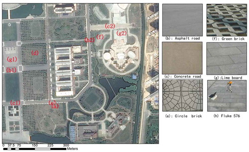
The in situ measurements of infrared temperature were conducted at the campus of Jiangxi Normal University, located in Nanchang, Jiangxi, South China. Five different impervious surfaces located at different experiment sites (Table 1) were selected in this study, i.e., asphalt road (Figure 1(b1,b2)), concrete road (Figure 1(c1,c2)), green bricks with “8” shape (Figure 1(e)), circle bricks (Figure 1(f)), and lime board (Figure 1(g)). The data for meteorological variables were collected by a regional automatic meteorological station (Beijing WH/ZQZ-A, China) located south of experiment sites (Figure 1(a)). Nanchang is located in the subtropical East Asian monsoon climate region. The prevailing wind direction is south-east during summer and north-west during winter. Therefore, wind conditions at the experiment sites should not be influenced by structures located west or east of the experiment sites.

Table 1. Characteristics of experiment sites.

Experiment sites	Biophysical characteristics
(b1)	Asphalt road from west to east, north of (b1) is covered by lime board and south of B1 is covered by grassland
(b2)	Asphalt road from south to north, east and west of road (b2) is covered by by grassland and shrub
(c1)	Concrete road from east to west, south of (c1) is a monument surrounded by separate pools; and north of (c1) is grassland
(c2)	Concrete road from east to west, northeast and northwest of (c2) are covered by lime board and grassland respectively
(e)	Circle bricks aside concrete road, north is asphalt road from south to north; south of (e) is the meteorological stations, surrounded by meadows
(f)	Green bricks with eight shapes, which situated the open environment
(g1) and (g2)	Both the lime board sites are located in the middle of open squares, covered by lime boards

Figure 1. Experiment sites of typical impervious surfaces: (a) situation of meteorological station; (b1) and (b2) Asphalt road; (c1) and (c2) Concrete road; (d) Grassland; (e) Circle brick; (f) Green brick; (g1) and (g2) lime board; (h) infrared thermometer (Fluke 576).

2.1.2. Infrared temperature data

A noncontact infrared thermometer (Fluke 576, Fluke Corporation, Everett, Washington D.C., USA) was used to measure the infrared temperature of impervious surfaces. The temperature range of the Fluke 576 is −30 ~900°C with an accuracy of ±0.75°C. The Fluke 576 was fixed to a tripod and connected to a computer to provide enough memory and power for continuous measurement of infrared temperature (Figure 1(h)). The distance of the equipment from impervious surfaces was approximately 50 cm. The measurements were conducted on 47 nonprecipitation days from October 15, 2012, to November 10, 2013. The infrared temperatures of impervious surfaces were collected eight times per second from sunrise to sunset. Only the measurement data collected on cloud-free days (Table 2) were used. Cloud-free (or clear) sky refers to zero cloud cover conditions throughout the day.

Table 2. Date, time, and volume for in situ measurement data collected under cloud-free conditions.

Impervious surfaces	Date	Local time	Data volume	EWS (m/s)	Experiment sites
Asphalt road	17 October 2012	10:35–21:15	103	0–11.5	(b1)
Asphalt road	18 October 2012	10:30–21:00	97	0–4.2	(b1)
Concrete road	12 May 2013	10:05–21:00	113	0–6.9	(c2)
Concrete road	13 May 2013	7:10–21:10	160	1.7–5.0	(c2)
Lime board	25 October 2013	7:50–20:45	197	4.0–9.5	(g2)
Lime board	13 November 2012	7:30–19:55	123	0–4.1	(g2)
Green brick	9 November 2013	7:15–21:30	160	0–5.6	(f)
Circle brick	22 May 2013	6:45–21:20	83	0–3.5	(e)

Note: The data volume is the number of measurement data at the frequency of 5 min.

2.1.3. Meteorological data

The meteorological data, including air temperature and wind direction and speed, were collected using an unmanned meteorological station, and observations were performed every 5 min. The wind properties were characterized by wind direction and speed at five time intervals, i.e., 2-min average wind speed and direction; 10-min average wind speed and direction; and maximum, extreme, and instantaneous wind speed, direction, and their generation time. Maximum wind speed was the maximum value of 10-min average wind speed in an hour. The hourly extreme wind speed (EWS) reported in each 5-min observation interval was the highest instantaneous wind speed for the most recent hour prior to the observation time. The maximum instantaneous wind speed decayed within a certain period of given EWS. The EWS was used to explore the relationship between wind speed and ITD over an hour. Cloud cover within a visible range from the experiment sites was recorded by a ground-based digital camera on the dates of measurement (Souza-Echer et al. 2006).

2.2. Methods

Figure 2 depicts a flowchart illustrating the methodology for estimating the influence of wind speed on infrared temperature of impermeable surfaces. First, infrared temperature data collected on cloudless days were selected. Subsequently, the averaged infrared temperature was calculated for each minute to eliminate abnormal measurement data. Finally, the postprocessing data were used to estimate ITD, explore the relationship between EWS and ITD by quantile regression, determine the primary ITD variable by comparison of Pearson correlation coefficient (Pr), and evaluate the impact duration of wind speed on ITD.

Figure 2. Methodology flowchart.

2.2.1. Estimation of ITD due to wind perturbations

2.2.1.1. Estimation of ITD

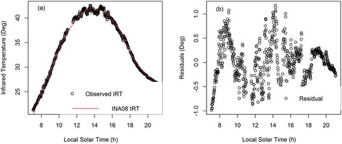
ITD for impervious surfaces was calculated by the residuals of infrared temperature. The residuals of infrared temperature were the difference between the observed infrared temperature and the predicted infrared temperature obtained from the DTC model. Infrared temperature measured on May 12, 2013, was taken as an example to calculate the ITD of concrete road (Figure 1(c2,c3). First, the normal DTC pattern of each impervious surface (Figure 3(a), red line) was simulated by INA08 (Equations (1)–(3)).

(1) $T_{day}\left(t\right)=T_0+T_a\mathrm{c}\mathrm{o}\mathrm{s}\left(\frac{\pi }{\omega }\left(t-t_m\right)\right),t<t_s$(1)

(2) $T_{night}\left(t\right)=\left(T_0+\delta T\right)+[T_a\mathrm{c}\mathrm{o}\mathrm{s}\left(\frac{\pi }{\omega }\left(t_s-t_m\right)-\delta T\right]\frac{k}{k+t-t_s},t\ge t_s$(2)

(3) $k=\frac{\omega }{\pi }\left[ta{n}^{-1}\left(\frac{\pi }{\omega }\left(t_s-t_m\right)\right)-\frac{\delta T}{T_a}si{n}^{-1}\left(\frac{\pi }{\omega }\left(t_s-t_m\right)\right)\right]$(3)

Figure 3. Example to estimate ITD of concrete road on 12 May 2013: (a) Observed infrared temperature (IRT) and modeled infrared temperature by INA08 (INA08 IRT); (b) Residual of infrared temperature. INA08 is the DTC model proposed by Inamdar et al. (2008).

here $T_{day}$ is the daytime temperature (°C); $T_{night}$ is the night temperature (°C); ω is the length of daylight hours (h); t is the observation time (h); k is the attenuation coefficient; π is the constant $\pi =3.1415927;T_0$ is the residual temperature at sunrise (°C); $T_a$ is the temperature amplitude (°C); $t_m$ is the time at which temperature reaches its maximum (h); $t_s$ is the starting time of free attenuation (h); and $\delta T$ is the temperature difference between $T_0$ and $\mathrm{T}\left(\mathrm{t}\to \mathrm{\infty }\right)$ (°C).

The ITD due to wind perturbations was estimated using the absolute value of infrared temperature residual. The INA 08 of individual impermeable surfaces was representative of the normal diurnal cycles of weather and biophysical parameters, such as air temperature, atmospheric pressure, humidity, precipitation, solar radiation, and intrinsic characteristics of the materials. Therefore, the regression parameters of INA 08 represented the weather and biophysical characteristics, while the infrared temperature residual of INA08 indicated the effects of wind speed fluctuation (Figure 3(b)). The plus or minus of the infrared temperature residual might be impacted by the wind direction. Infrared temperature residuals on May 12, 2013, shifted from positive (~8:00 AM) to negative (~12:00 PM) under the influence of the north-west wind, while a shift from negative (~12:00 PM) to positive (~14:00 PM) was observed at the experiment site of (c2) under the influence of the north-east wind. The residual shifts were caused by changes in land-use/cover patterns in the north-west and north-east regions. The north-west of (c2) was characterized as a grassland, and the infrared temperature at this site was less than that of the concrete road. The north-east of (c2) was marble and indicated a temperature higher than the concrete road (Figure 1). The extreme value of the residual occurred when the EWS reached the maximum value within a certain period of unchanged wind direction. For example, the extreme residual value occurred during the period from ~13:00 PM to 15:00 PM, when the EWS over 5-min intervals reached the maximum value. The absolute value of the infrared temperature residual was deemed as the ITD due to wind perturbation.

2.2.1.2. ITD statistical measures

The ITD is not a constant but is distributed continuously under the impact of EWS (Figure 4). Several statistical indexes were calculated to improve its evaluability with regard to the influence of wind speed. These indexes included range (Equation (4)), standard deviation (Equation (5)), mean, and quantiles. Consistent with the frequency of wind speed, the variability of ITD over 5-min intervals was calculated. Five quantiles of ITD, i.e., 10%, 25%, 50%, 75%, and 90%, were determined.

(4) $T_{ra}=T_{max}-T_{min}$(4)

Figure 4. Residual (0.2 Deg.) distribution under the influence of extreme wind speed (EWS) and direction (EWD) at the site (c2) on 12 May 2013: arrow represents the wind direction and the size of the arrow is the wind speed with the unit 0.1 m s^−1.

where $T_{ra}$ is the range of ITD (ITD_RA) over 5-min intervals (°C); $T_{max}$ is the maximum value of ITD (ITD_MAX) over 5-min intervals (°C); and $T_{min}$ is the minimum value of ITD (ITD_MIN) over 5-min intervals (°C).

(5) $T_{sd}=\sqrt{\frac{{\sum }_{i=1}^5{\left(T_i-\bar{T}\right)}^2}{4}}$(5)

where $T_{sd}$ is the standard deviation of ITD (°C); $\left\{T_1,T_2,\cdots ,T_5\right\}$ are the observed ITD values over 5-min intervals (°C); and $\bar{T}$ is the mean of the observed ITD values over 5-min intervals (°C).

2.2.2. Relationship between EWS and ITD using quantile regressions

The quantile regression method was used to define the relationship between wind speed and ITD. Quantile regression (Koenker and Bassett 1978) is a method for estimating functional relations between variables for all portions of a probability distribution. It is particularly suitable for skewed response distributions (i.e., the predictor variables exert a significant impact on both the change in mean and change in the variance of the distribution). Therefore, this method was appropriate for determining the limiting relationships between wind speed and ITD, where wind speed was the predictor variable and ITD was the dependent variable (Cade, Terrell, and Schroeder 1999; Dunham, Cade, and Terrell 2002; Muggeo et al. 2013). Details of regression quantile modeling have been reported elsewhere (Cade, Terrell, and Schroeder 1999).

The best model form and the primary ITD variable should be determined to select the ideal quantile regression model. Both linear and nonlinear quantile regression models were considered to determine the best model form (Cade and Noon 2003; Haque, Nehrir, and Mandal 2014; Juban et al. 2016). Scatter-plot matrices were used to examine the relationships between the ITD statistical measures and between the EWS and ITD statistical measures. Pearson correlation coefficients (Pr) of the EWS and ITD statistical measures were compared to determine the dominant ITD statistical measures, which were significantly correlated with the EWS (Section 3). The regression quantile coefficient of determination (R¹, not R²) for the five quantile values of $\tau$ ($\tau$ = 0.1, 0.25, 0.5, 0.75, 0.9) was used to determine the primary ITD variable for the selected quantile regression model. The general formula for the regression quantile coefficient of determination is ${\mathrm{R}}^1=1-\mathrm{F}\left(\tau \right)/\mathrm{R}\left(\tau \right)$, where $\mathrm{F}\left(\tau \right)$ is the weighted sum of absolute deviations minimized in estimating a full-parameter model and $\mathrm{R}\left(\tau \right)$ is the weighted sum of absolute deviations minimized for estimating the reduced-parameter model for any $\tau$ (Koenker and Machado 1999; Dunham, Cade, and Terrell 2002).

The regression coefficients across quantiles were incorporated into the model to provide an estimate with less sampling variation (Cade and Noon 2003). The intercept variation across quantiles indicated the ITD variation at the minimum wind speed in a day. The change in slope across quantiles indicated the distribution patterns of ITD statistical measures. Homogeneous distributions implied an equal variation of ITD statistical measures for all quantiles and resulted in regression quantile slope estimates that were nearly parallel. Heterogeneous distributions implied an unequal variation of ITD statistical measures and resulted in regression quantile slope estimates that were not parallel (Dunham, Cade, and Terrell 2002; Terrell et al. 1996).

2.2.3. Impact duration of EWS on ITD

After determining the best model form and estimating the regression quantiles for ITD of impervious surfaces, a probabilistic prediction interval was constructed to evaluate the influence of EWS on the magnitude of ITD over a period of an hour. Various points of a univariate one-sample distribution were described by estimating different quantiles of the cumulative distribution function. The ${\tau }^{\mathrm{t}\mathrm{h}}$ quantile estimate provided a proportion ($\tau$) of the observation samples less than or equal to the estimate (Cade, Terrell, and Schroeder 1999). For example, the 0.9th quantile was an estimate such that 90% of the observed ITD statistical measures were less than or equal to the estimated ITD statistical measures. In this study, the 0.9th quantile was deemed to exhibit the maximum impact of EWS on ITD statistical measures, while the 0.1th quantile indicated the minimum impact of EWS on the ITD statistical measures over the duration of an hour (Section 3). An 80% prediction interval was constructed from the 0.1th to the 0.9th regression quantiles to predict the magnitude of ITD statistical measures over an hour (Equation (6)).

(6) $D_v^i=T_{vmax}^i-T_{vmin}^i$(6)

where $D_v^i$ is the decay magnitude of the ITD statistical measures at the given EWS for the $\mathrm{i}\mathrm{t}\mathrm{h}$ impervious surface and is indicated as the difference between the maximum ($T_{vmax}^i$) and minimum ($T_{vmin}^i$) impacts of EWS on the ITD variable for the $\mathrm{i}\mathrm{t}\mathrm{h}$ impervious surface. The units of the ITD statistical measures are degree Celsius (°C).

The impact duration of EWS on ITD was calculated as the ratio of the maximum impact of EWS and the decay magnitude of ITD statistical measures over an hour (Equation (7)).

(7) $D{T}_i=\frac{T_{vmax}^i}{D_v^i}$(7)

where $D{T}_i$ is the impact duration time of ITD for the $i\mathrm{t}\mathrm{h}$ impervious surface; $T_{vmax}^i$ is the maximum influence of EWS on the ITD statistical measures for the $\mathrm{i}\mathrm{t}\mathrm{h}$ impervious surface; and $D_v^i$ is the decay magnitude of the ITD statistical measures for the $i\mathrm{t}\mathrm{h}$ impervious surface over an hour.

3. Results

3.1. Best regression quantile model and the primary dominant variable

Wedge-shaped and exponential distribution patterns were observed between the EWS and ITD statistical measures (Figure 6). The exponential quantile regression equation (Equation (8)) was determined as the best model form to estimate the influence of wind speed on ITD statistical measures.

(8) $T_v^i=m_v^i\ast e^{c_v^i\ast w}$(8)

where $T_v^i$ is one of the ITD statistical measures (Section 2.2.2) for the $i\mathrm{t}\mathrm{h}$ impervious surface (°C); $w$ is the EWS of the last hour with unit of m s⁻¹; $m_v^i$ and $c_v^i$ are free parameters of the exponential quantile regression for the $i\mathrm{t}\mathrm{h}$ impervious surface.

ITD_RA, a single number representing the spread of ITD, was determined as the primary variable. ITD_MAX and ITD_RA were determined as the dominant statistical indexes as indicated by the scatter plots between the ITD statistical measures (Figure 5) and the comparison among Pearson correlation coefficients of EWS and ITD statistical measures (Pr in Figure 6). ITD_MAX indicated significant linear correlations with other quantile values of ITD (inc., minimum of ITD (ITD_MIN), 25% of ITD (ITD_25%), 50% of ITD (ITD_50%), and 75% of ITD (ITD_75%)). ITD_RA was significantly correlated with a standard derivation of ITD (ITD_SD) (Figure 5). Both ITD_MAX and ITD_RA were significantly correlated with EWS (Figure 6) and were retained as the dominant statistical indexes. Additionally, the relationships between EWS and the dominant statistical indexes of ITD were examined by exponential regression quantiles for individual impervious surfaces, i.e., asphalt, concrete, lime, and bricks. A robust relationship existed between ITD_RA and EWS. However, ITD_MAX was not robustly related to the EWS under varying wind direction conditions (Figure 7). Therefore, the ITD changed within a range during the time period of a given EWS.

Figure 5. Scatter-plot matrices among ITD statistical measures. ITD statistical measures include five quantiles of ITD (i.e., minimum of ITD (ITD_MIN), 25% of ITD (ITD_25%), 50% of ITD (ITD_50%), 75% of ITD (ITD_75%) and maximum ITD (ITD_MAX)), mean (ITD_MN), range (ITD_RA) and standard derivation of ITD (ITD_SD).

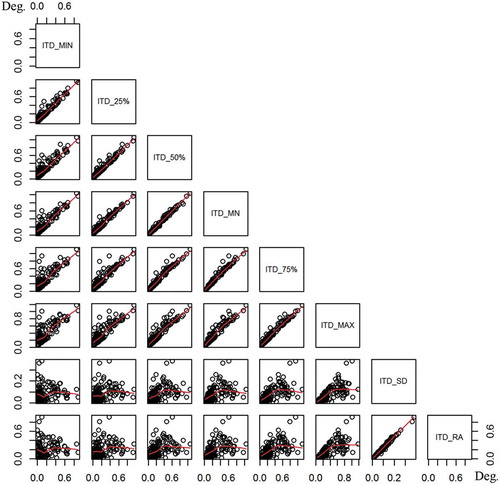
Figure 6. Scatter-plot matrices for EWS and ITD statistical measures on 12 May 2013, statistical measures include five quantiles of ITD (i.e., minimum of ITD (ITD_MIN), 25% of ITD (ITD_25%), 50% of ITD (ITD_50%), 75% of ITD (ITD_75%) and maximum ITD (ITD_MAX)), mean (ITD_MN), range (ITD_RA) and standard derivation (ITD_SD) of ITD. Pr is the Pearson correlation coefficient of ITD statistical measures and EWS.

Figure 7. Coefficients of determination (R¹) between EWS and ITD_MAX (EWS-ITD_MAX), and between EWS and ITD_RA (EWS-ITD_RA) for exponential regression quantiles at five values of $\tau$ (i.e., 0.1, 0.25, 0.5, 0.75 and 0.9).

3.2. Effects of EWS on ITD_RA

The estimated ITD_RA at the minimum wind speed (intercept m) differed among the impermeable surfaces and changed with EWS. The estimated ITD_RA for impervious surfaces at the 0.75th quantile was less than ~0.1 under nonwind conditions and less than ~0.2 when the EWS was up to 2.0 m s⁻¹ (Figure 8). The estimated ITD_RA at the 0.9th quantile increased sharply with an increase in the EWS, especially when EWS was greater than 2.0 m s⁻¹. The estimated ITD_RA at the 0.9th quantile was greatest for circle bricks, when EWS increased from 2.0 to 3.5 m s⁻¹, followed by asphalt, concrete, lime board, and green bricks. For asphalt and concrete, estimated ITD_RA at the 0.9th quantile has little difference between different measurement dates under the same value of EWS (e.g., EWS =5 m s⁻¹) (Figure 8). Otherwise for lime board, the estimated ITD_RA at the 0.9th quantile on 13 November 2012 was much larger than that on 25 October 25 2013, when the EWS is equal to 4 ms⁻¹. For lime board, the 0.9th estimated ITD_RA at the minimum EWS on 25 October 2013 (EWS =4 m s⁻¹) was approximately equal to that at the minimum EWS on 13 November 2012 (EWS =0 ms⁻¹). Therefore, the relative EWS might be the dominant contributors for the influence of EWS on ITD_RA. For a special impervious surface, ITD samples on different dates were combined to explore the relationship between ITD and relative EWS. The regression quantile analysis was conducted between the ITD_RA and the relative EWS for the impermeable surfaces (Figure 9).

Figure 8. Regression quantiles for range of ITD (ITD_RA) and extreme wind speed (EWS) at five values (red = 0.1; green = 0.25, blue = 0.5, orange = 0.75, purple = 0.9): Asphalt on 17 October 2012 and 18 October 2012; Concrete on 12 May 2013 and 13 May 2013; Lime board on 25 October 2013 and 13 November 2012; Green brick on 9 November 2013; Circle brick on 22 May 2013.

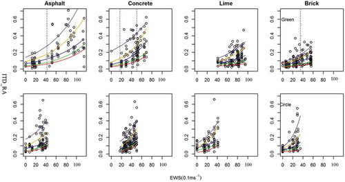
Figure 9. Regression quantiles for range of ITD (ITD_RA) and relative extreme wind speed (EWS) at five values (red = 0.1; green = 0.25, blue = 0.5, orange = 0.75, purple = 0.9) and the regression coefficients at quantile value of 0.9.

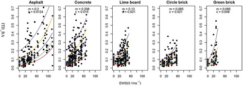
Both the estimated intercepts at the minimum EWS (m) and slopes (c) were differed among the impermeable surfaces. If the natural logarithm of ITD_RA was determined as the dependent variable, the free parameters (m and c) were the intercept and slope of regression quantiles, respectively. The estimated intercepts at the minimum EWS (m) for asphalt was approximately equal to that for concrete, followed by lime board, and bricks (inc. circle and green brick). The intercept m for circle brick is equal to that for green brick. The estimated slope for green bricks (c =0.048) got the maximum value, followed by that for lime board and circle brick (c =0.021), concrete (c =0.015), and asphalt (c =0.012).

3.3. Impact duration of EWS on ITD_RA

An 80% prediction model was constructed to estimate the magnitude of ITD resulting from relative wind speed fluctuations over an hour duration. The prediction models for impervious surfaces such as asphalt, concrete, and lime board were approximately homogeneous between different measurement dates (open and closed circles in Figure 12). The ITD_RA was the decay magnitude over 5-min intervals and was mainly influenced by the relative EWS (and not the absolute EWS). The 80% prediction model for a particular surface was retrieved from the relative EWS (lines in Figure 10). Equation (8) was used as the prediction model form.

Figure 12. Coefficient testing for regression quantiles at five values of $\tau$ (0.1, 0.25, 0.5, 0.75, 0.9) to analyze the relationship between range of ITD (ITD_RA) and relative extreme wind speed (EWS). m and c are the coefficients of regression quantiles; m.t and c.t are t test value for the coefficient of m and c, respectively; m.p and c.p are the p values for coefficient of m and c, respectively.

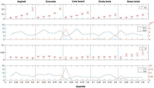
Figure 10. 80% prediction lines and correlation coefficient between prediction values and 80% ITD intervals (i.e., difference between 0.1th and 0.9th regression quantiles) on different dates. EWS is the extreme wind speed with the unit of m s^−1.

The magnitude of ITD over an hour increased with increasing EWS, and the estimated slope of ITD_RA (c in Figure 10) was influenced by the impervious surface type. The estimated slopes of ITD_RA for asphalt and concrete were approximately equal. Circle bricks indicated the highest estimated slope of ITD_RA, followed by green bricks, lime board, and concrete road.

The influence of EWS on ITD_RA lasted more than 1.3 h for impervious surfaces and the impact duration increased with increase in relative EWS (Table 3). Additionally, the maximum impact of EWS on ITD_RA was estimated by the exponential quantile regression between ITD_RA and the relative EWS (Figure 9). Subsequently, the impact duration was calculated as a function of the relative EWS (Table 3). The impact duration was greater than 1.3 h and varied with the type of impervious surface if the relative EWS values were equal (Table 3). The impact duration differences among different impervious surfaces might cause abnormal spatial patterns of infrared temperature in urban areas.

Table 3. Duration for the influence of EWS on ITD_RA for impervious surfaces.

Types	Duration (Unit: hour)
Asphalt	$\mathrm{D}\mathrm{T}=1.33{\mathrm{e}}^{0.0002w}$
Concrete	$\mathrm{D}\mathrm{T}=1.31{\mathrm{e}}^{0.0004w}$
Lime	$\mathrm{D}\mathrm{T}=1.34{\mathrm{e}}^{0.0023w}$
Circle brick	$\mathrm{D}\mathrm{T}=1.43{\mathrm{e}}^{0.0257w}$
Green brick	$\mathrm{D}\mathrm{T}=1.34{\mathrm{e}}^{0.0267w}$

Note: $w$ is the relative EWS with unit of 0.1 m s⁻¹.

4. Discussion

4.1. Impact factor analysis

The variation of estimated intercept (m in Figure 11) and the variation of estimated slope (c in Figure 11) might be impacted by both wind conditions and the impermeable surfaces. The variation of the intercept under conditions of sustained wind speed (13 May 2013) was not greater than that during nonsustained wind speed conditions (12 May 12 2013) (m in Figure 11). There was no significant correlation between the variation of the intercept (m in Figure 11) and the variation of the EWS (Table 2) for individual impervious surfaces. The variation of the intercept at lower wind speeds was different for different impervious surfaces. Asphalt indicated the highest variation of the intercept, followed by concrete, lime board, and bricks. The differences among the impermeable surfaces were influenced by the intrinsic characteristics of the materials (e.g., surface roughness). The rougher the surface, the higher the variation of the intercept. Therefore, the variation of estimated intercept (m) was impacted by the impermeable surface types.

Figure 11. Coefficient testing for regression quantiles at five values of $\tau$ (0.1, 0.25, 0.5, 0.75, 0.9) to analyze the relationship between the range of ITD (ITD_RA) and extreme wind speed (EWS). m and c are the coefficients of regression quantiles; m.t and c.t are t test value for the coefficient of m and c,respectivelyc; m.p and c.p are the p value for coefficient of m and c, respectivelyc.

Heterogeneous distributions were obtained for the estimated ITD_RA due to wind speed fluctuations over 5-min intervals. The maximum slopes with regard to regression quantiles (c) changed with the surface types: (1) the maximum slopes for asphalt and concrete roads occurred at the 0.1th quantile; (2) the maximum slope for lime board changed with the wind speed conditions and the 0.1th quantile slope indicated the maximum value under nonsustained wind speed conditions (13 November 2012), while the 0.75th quantile slope was the highest under sustained wind speed conditions (25 October 2013); (3) little difference was observed among the five $\tau$ values for the green bricks (higher friction); and (4) the maximum slope for the circle bricks (lower friction) occurred at 0.9th quantile (c in Figure 11). Therefore, the variation of slopes across regression quantiles was impacted by both wind conditions and impermeable surface types.

Under consistent wind conditions, the variation of slopes could be attributed to the ITD sample size and the intrinsic characteristics of the materials (e.g., thermal conductivity and surface roughness). The variation of slopes across five quantiles, retrieved from regression quantile analysis between ITD and relative EWS (c in Figure 12), is much less than that between ITD and EWS (c in Figure 11). The variation of slopes, as indicated in Figures 11 and 12, could be attributed to the ITD sample size (Section 3). The estimated slopes of asphalt and concrete indicated a decreasing trend with increasing quantile values ($\tau$). A small increasing trend was observed for the estimated slopes of lime board and green bricks. There was little change in the estimated slope of circle bricks for the five quantile values.

4.2. Uncertainty analysis

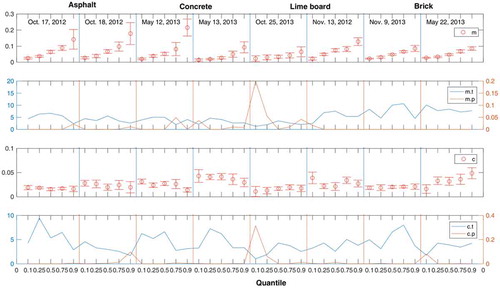
The estimated coefficients (m and c) were highly significant (P < 0.005) for most of the impermeable surface types (Figure 11). Nonsignificant intercept (m) values for the 0.1th, 0.25th, and 0.9th quantiles were observed for lime board on 25 October 2013 and for the 0.75th quantile for concrete road on 12 May 2013. Four estimated slopes (c) were not significant, i.e., the estimated 0.9th quantile slope for asphalt on 18 October 2012, the estimated 0.1^th and 0.25^th quantile slopes for lime board on 25 October 2013, and the estimated 0.1th quantile slope for circle bricks on 22 May 2013 (Figure 11). The nonsignificant intercept and slope values, especially for the 0.1th quantile, could be attributed to the sustained wind speed on 25 October 2013. The other nonsignificant estimated m and c values could be attributed to a small sample size (Figures 8 and 9), and these values became significant when the sample size was increased (Figures 11 and 12).

The 80% prediction model achieved high significance for all impermeable surfaces except for lime board under conditions of sustained wind speeds. The statistical significance of model parameters (m and c) indicated its statistical validity. The 80% prediction model was based on the 0.1th and 0.9th quantiles and achieved high validity for different materials. The prediction models for different materials were significantly correlated with the 80% prediction interval (i.e., difference between the 0.1th and 0.9th quantiles) (Figure 10). The 80% prediction model indicated high significance for all surfaces under conditions of nonsustained wind speeds.

5. Conclusions

This study developed a technical scheme for evaluation of wind speed effects on infrared temperature. The application of in situ measurements and online infrared thermometer provided a reliable technique to determine the infrared temperatures of individual impervious surfaces at high frequency. The residual-based method adopted from the DTC model was efficient in estimating the ITD due to fluctuating wind speed. The exponential regression quantile equation was established as the best model for determining the relationship between fluctuating wind speed and the ITD. Additionally, the probabilistic prediction interval and the ratio method provided feasible and quantitative methods to estimate the influence of wind perturbation on the ITD.

The results of this study allow the selection of reliable thermal images for drawing scientific conclusions and help evaluate scientific outputs from thermal remote-sensing applications. Unreliable research conclusions might be drawn from thermal remote-sensing applications if the images are acquired in fluctuating wind conditions. For example, the differences in decay magnitude, rate, and duration might result in abnormal spatial patterns of infrared temperatures for impervious surfaces in urban areas. Future research in this regard should focus on estimating the threshold of wind speed which results in such abnormal spatial patterns. In this study, only impervious surfaces were selected and future research should consider other land surface types to determine the threshold of wind speed. The results also indicated that the sample size affected the regression coefficients of different quantiles. Moreover, the intrinsic characteristics of the materials as well as the land surface patterns significantly affected the ITD, and this should be further investigated. Additionally, the influence of wind direction should also be studied.

The results of the present study could be utilized for correcting thermal infrared images of homogeneous surfaces. However, the wind direction and land surface type must be considered for correcting images of heterogeneous surfaces.

Acknowledgements

This study was supported by the Natural Science Foundation of China [41461079, 41101341] and the China Scholarship Council [201708360054].

Disclosure statement

No potential conflict of interest was reported by the authors.

Additional information

Funding

This work was supported by the China Scholarship Council [201708360054];National Natural Science Foundation of China [41461079];

References

- Allison, R., J. Johnston, G. Craig, and S. Jennings. 2016. “Airborne Optical and Thermal Remote Sensing for Wildfire Detection and Monitoring.” Sensors 16 (8): 1310 (1–29). doi:10.3390/s16081310.
- Astarita, T., G. Cardone, and G. M. Carlomagno. 2006. “Infrared Thermography: An Optical Method in Heat Transfer and Fluid Flow Visualization.” Optics and Lasers in Engineering 44 (3–4): 261–281. doi:10.1016/j.optlaseng.2005.04.006.
- Balageas, D. L., D. M. Boscher, and A. A. Deom. 1990. “Measurement of Convective Heat-Transfer Coefficients on a Wind Tunnel Model by Passive and Stimulated Infrared Thermograpy.” In Proc. SPIE 1341, Infrared Technology XVI, November 1. doi: 10.1117/12.23107.
- Bhuiyan, C., A. K. Saha, N. Bandyopadhyay, and F. N. Kogan. 2017. “Analyzing the Impact of Thermal Stress on Vegetation Health and Agricultural Drought–A Case Study from Gujarat, India.” GIScience & Remote Sensing 54 (5): 678–699. doi:10.1080/15481603.2017.1309737.
- Blocken, B., T. Stathopoulos, and J. P. A. J. van Beeck. 2016. “Pedestrian-Level Wind Conditions around Buildings: Review of Wind-Tunnel and CFD Techniques and Their Accuracy for Wind Comfort Assessment.” Building and Environment 100 (May): 50–81. doi:10.1016/j.buildenv.2016.02.004.
- Cade, B., J. Terrell, and R. Schroeder. 1999. “Estimating Effects of Limiting Factors with Regression Quantiles.” Ecology 80 (1): 311–323. doi:10.1890/0012-9658(1999)080[0311:EEOLFW]2.0.CO;2.
- Cade, B. S., and B. R. Noon. 2003. “A Gentle Introduction to Quantile Regression for Ecologists.” Frontiers in Ecology and the Environment 1 (8): 412–420. doi:10.1890/1540-9295(2003)001[0412:AGITQR]2.0.CO;2.
- Carlomagno, G. M. 1997. “Thermo-Fluid-Dynamic Applications of Quantitative Infrared Thermography.” Journal of Flow Visualization and Image Processing 4 (3): 261–280. doi:10.1615/JFlowVisImageProc.v4.i3.70.
- Chen, X. L., H. M. Zhao, P. X. Li, and Z. Y. Yin. 2006. “Remote Sensing Image-Based Analysis of the Relationship between Urban Heat Island and Land Use/Cover Changes.” Remote Sensing of Environment 104 (2): 133–146. doi:10.1016/j.rse.2005.11.016.
- Cook, N. J., P. Chan, D. Wu, and M. A. Holder. 2002. “Towards Quantitative Visualisation of Transient Surface Flow on Building Models Using Infrared Thermography.” Journal of Wind Engineering and Industrial Aerodynamics 90 (6): 663–673. doi:10.1016/S0167-6105(02)00154-X.
- Duan, S. B., Z. L. Li, B. H. Tang, H. Wu, and R. L. Tang. 2014. “Direct Estimation of Land-Surface Diurnal Temperature Cycle Model Parameters from MSG–SEVIRI Brightness Temperatures under Clear Sky Conditions.” Remote Sensing of Environment 150: 34–43. doi:10.1016/j.rse.2012.04.016.
- Duan, S. B., Z. L. Li, N. Wang, H. Wu, and B. H. Tang. 2012. “Evaluation of Six Land-Surface Diurnal Temperature Cycle Models Using Clear-Sky in Situ and Satellite Data.” Remote Sensing of Environment 124: 15–25. doi:10.1016/j.rse.2012.04.016.
- Dunham, J., B. Cade, and J. Terrell. 2002. “Influences of Spatial and Temporal Variation on Fish-Habitat Relationships Defined by Regression Quantiles.” Transactions of the American Fisheries Society 131 (1): 86–98. doi:10.1577/1548-8659(2002)131<0086:IOSATV>2.0.CO;2.
- Frey, C. M., and E. Parlow. 2012. “Flux Measurements in Cairo. Part 2: On the Determination of the Spatial Radiation and Energy Balance Using ASTER Satellite Data.” Remote Sensing 4 (9): 2635–2660. 2635–2660. doi:10.3390/rs4092635.
- Göttsche, F. M., and F. S. Olesen. 2001. “Modelling of Diurnal Cycles of Brightness Temperature Extracted from METEOSAT Data.” Remote Sensing of Environment 76 (3): 337–348. doi:10.1016/S0034-4257(00)00214-5.
- Göttsche, F. M., and F. S. Olesen. 2009. “Modelling the Effect of Optical Thickness on Diurnal Cycles of Land Surface Temperature.” Remote Sensing of Environment 113 (11): 2306–2316. doi:10.1016/j.rse.2009.06.006.
- Haack, T., S. D. Burk, and R. M. Hodur. 2005. “US West Coast Surface Heat Fluxes, Wind Stress, and Wind Stress Curl from a Mesoscale Model.” Monthly Weather Review 133 (11): 3202–3216. doi:10.1175/MWR3025.1.
- Haque, A. U., M. H. Nehrir, and P. Mandal. 2014. “A Hybrid Intelligent Model for Deterministic and Quantile Regression Approach for Probabilistic Wind Power Forecasting.” IEEE Transactions on Power Systems 29 (4): 1663–1672. doi:10.1109/TPWRS.2014.2299801.
- Hartz, D. A., L. Prashad, B. C. Hedquist, J. Golden, and A. J. Brazel. 2006. “Linking Satellite Images and Hand-Held Infrared Thermography to Observed Neighborhood Climate Conditions.” Remote Sensing of Environment 104 (2): 190–200. doi:10.1016/j.rse.2005.12.019.
- Holmes, T. R. H., W. T. Crow, C. Hain, M. C. Anderson, and W. P. Kustas. 2015. “Diurnal Temperature Cycle as Observed by Thermal Infrared and Microwave Radiometers.” Remote Sensing of Environment 158: 110–125. doi:10.1016/j.rse.2014.10.031.
- Hoyano, A., K. Asano, and T. Kanamaru. 1999. ““Analysis of the Sensible Heat Flux from the Exterior Surface of Buildings Using Time Sequential Thermography.” Atmospheric Environment 33 (24): 3941–3951. doi:10.1016/S1352-2310(99)00136-3.
- Inamdar, A., A. French, S. Hook, G. Vaughan, and W. Luckett. 2008. “Land Surface Temperature Retrieval at High Spatial and Temporal Resolutions over the Southwestern United States.”.” Journal of Geophysical Research 113 (D7): 1–18. doi:10.1029/2007JD009048.
- Jiang, G. M., Z. L. Li, and F. Nerry. 2006. “Land Surface Emissivity Retrieval from Combined Mid-Infrared and Thermal Infrared Data of MSG-SEVIRI.” Remote Sensing of Environment 105 (4): 326–340. doi:10.1016/j.rse.2006.07.015.
- Juban, R., H. Ohlsson, M. Maasoumy, L. Poirier, and J. Z. Kolter. 2016. “A Multiple Quantile Regression Approach to the Wind, Solar, and Price Tracks of GEFCom2014.” International Journal of Forecasting 32 (3): 1094–1102. doi:10.1016/j.ijforecast.2015.12.002.
- Koenker, R., and G. Bassett. 1978. “Regression Quantiles.” Econometrica 46 (1): 33–50. doi:10.2307/1913643.
- Koenker, R., and J. A. F. Machado. 1999. “Goodness of Fit and Related Inference Processes for Quantile Regression.” Journal of the American Statistical Association 94: 1296–1310. doi:10.1080/01621459.1999.10473882.
- Lehmann, B., W. K. Ghazi, T. Frank, B. V. Collado, and C. Tanner. 2013. “Effects of Individual Climatic Parameters on the Infrared Thermography of Buildings.” Applied Energy 110: 29–43. doi:10.1016/j.apenergy.2013.03.066.
- Liou, Y., and S. Kar. 2014. “Evapotranspiration Estimation with Remote Sensing and Various Surface Energy Balance Algorithms—A Review.” Energies 7 (5): 2821–2849. doi:10.3390/en7052821.
- Luca, L. D., G. Cardone, G. M. Carlomagno, D. A. Chevalerie. 1992. “Flow Visualization and Heat Transfer Measurements in Hypersonic Wind Tunnel.” Experimental Heat Transfer 5 (1): 65–78. doi:10.1080/08916159208946433.
- Mostovoy, G. V., R. L. King, K. R. Reddy, V. G. Kakani, and M. G. Filippova. 2006. “Statistical Estimation of Daily Maximum and Minimum Air Temperatures from MODIS LST Data over the State of Mississippi.” GIScience & Remote Sensing 43 (1): 78–110. doi:10.2747/1548-1603.43.1.78.
- Muggeo, V., M. Sciandra, A. Tomasello, and S. Calvo. 2013. “Estimating Growth Charts via Nonparametric Quantile Regression: A Practical Framework with Application in Ecology.” Environmental and Ecological Statistics 20 (4): 519–531. doi:10.1007/s10651-012-0232-1.
- Nakamura, H., and S. Yamada. 2013. “Quantitative Evaluation of Spatio-Temporal Heat Transfer to a Turbulent Air Flow Using a Heated Thin-Foil.” International Journal of Heat and Mass Transfer 64: 892–902. doi:10.1016/j.ijheatmasstransfer.2013.05.006.
- Savage Shannon, L., L. Lawrence Rick, G. Custer Stephan, T. Jewett Jeffrey, L. Powell Scott, and J. A. Shaw. 2010. “Review of Alternative Methods for Estimating Terrestrial Emittance and Geothermal Heat Flux for Yellowstone National Park Using Landsat Imagery.” GIScience & Remote Sensing 47: 460–470. doi:10.2747/1548-1603.47.4.460.
- Singh, P., N. Kikon, and P. Verma. 2017. “Impact of Land Use Change and Urbanization on Urban Heat Island in Lucknow City, Central India. A Remote Sensing Based Estimate.” Sustainable Cities and Society 32: 100–114. doi:10.1016/j.scs.2017.02.018.
- Souza-Echer, M. P., E. B. Pereira, L. S. Bins, and M. A. R. Andrade. 2006. “A Simple Method for the Assessment of the Cloud Cover State in High-Latitude Regions by A Ground-Based Digital Camera.” Journal of Atmospheric and Oceanic Technology 23 (3): 437–447. doi:10.1175/JTECH1833.1.
- Sun, D., and R. Pinker. 2005. “Implementation of GOES-Based Land Surface Temperature Diurnal Cycle to AVHRR.” International Journal of Remote Sensing 26 (18): 3975–3984. doi:10.1080/01431160500117634.
- Terrell, J. W., B. S. Cade, J. Carpenter, and J. M. Thompson. 1996. “Modelling Stream Fish Habitat Limitations from Wedge-Shaped Patterns of Variation in Standing Stock.” Transactions of the American Fisheries Society 125: 104–117. doi:10.1577/1548-8659(1996)125<0104:msfhlf>2.3.co;2.
- Tsang, L., T. Liao, S. Tan, H. Huang, T. Qiao, and K. Ding. 2017. “Rough Surface and Volume Scattering of Soil Surfaces, Ocean Surfaces, Snow, and Vegetation Based on Numerical Maxwell Model of 3-D Simulations.” IEEE Journal of Selected Topics in Applied Earth Observations and Remote Sensing 10 (11): 4703–4720. doi:10.1109/JSTARS.2017.2722983.
- Van Den Bergh, F., M. A. Van Wyk, and B. J. Van Wyk. 2006. “Comparison of Data-Driven and Model-Driven Approaches to Brightness Temperature Diurnal Cycle Interpolation.” In Presented at the17th Annual Symposium of the Pattern Recognition Association of South Africa, Parys, South Africa, November 29–December 29–December 1. http://hdl.handle.net/10204/991.
- Vondou, D. A., A. Nzeukou, and F. M. Kamga. 2010. “Diurnal Cycle of Convective Activity over the West of Central Africa Based on Meteosat Images.” International Journal of Applied Earth Observation and Geoinformation 12 (Sup. 1): S58–S62. doi:10.1016/j.jag.2009.09.011.
- Weng, Q., and P. Fu. 2014. “Modeling Diurnal Land Temperature Cycles over Los Angeles Using Downscaled GOES Imagery.” ISPRS Journal of Photogrammetry and Remote Sensing 97: 78–88. doi:10.1016/j.isprsjprs.2014.08.009.
- Wu, H., and T. Stathopoulos. 1997. “Application of Infrared Thermography for Pedestrian Wind Evaluation.” Journal of Engineering Mechanics 123 (10): 978–985. doi:10.1061/(ASCE)0733-9399(1997)123:10(978).
- Yamada, M., Y. Uematsu, and T. Koshihara. 1988. “Visualization of the Flow around a Two-Dimensional Circular Cylinder by Means of Infrared Thermography (Part 1 Smooth Cylinder).” Wind Engineers, JAWE 35: 35–44. (in Japanese with English summary). doi:10.5359/jawe.1988.35_35.
- Yamada, M., Y. Uematsu, and R. Sasaki. 1996. “A Visual Technique for the Evaluation of the Pedestrian-Level Wind Environment around Buildings by Using Infrared Thermography.”.” Journal of Wind Engineering and Industrial Aerodynamics 65 (1): 261–271. doi:10.1016/S0167-6105(97)00045-7.
- Zhang, D., and G. Zhou. 2016. “Estimation of Soil Moisture from Optical and Thermal Remote Sensing: A Review.” Sensors 16 (8): 1308 (1–29). doi:10.3390/s16081308.
- Zhang, Y., T. He, S. Liang, D. Wang, and Y. Yu. 2018. “Estimation of All-Sky Instantaneous Surface Incident Shortwave Radiation from Moderate Resolution Imaging Spectroradiometer Data Using Optimization Method.” Remote Sensing of Environment 209 (May): 468–479. doi:10.1016/j.rse.2018.02.052.