A geospatial study of the drought impact on surface water reservoirs: study cases from Texas, USA

Abstract

Satellite images have been used historically to measure and monitor fluctuations in the surface water reservoirs. This study integrates remote sensing and Geographic Information System (GIS) technologies to investigate the impact of drought on 10 selected surface water reservoirs in San Angelo and Dallas, Texas. Oscillations in summer and winter months throughout the 2005–2016 period were assessed using multispectral images from Landsat-5, −7, and −8, and changes in the reservoirs were characterized and correlated against local climate data of each reservoir. For quantitative comparisons of the time-series measurements, a robust density slicing approach was employed to classify the range of values of the raster cells in the near-infrared band of Landsat images for each lake into three desired classes (deep water, shallow water, and dry area) based on the natural breaks inherent in the dataset. Statistical analysis shows that the overall accuracy of the classification is about 94%, which demonstrates the efficiency of the density slicer to accurately estimate surface water area changes from an individual Landsat band. Shrinkage in the surface water area over the study period reveals the concrete impact that the drought along with other factors have on the 10 selected lakes. The San Angelo lakes located in west central Texas experienced a nearly consistent pattern of change during most of the study period; whereas the Dallas lakes in northeast Texas followed the oscillating pattern of drought and correlated closely to the local conditions. Shockingly, the extreme drought caused complete vanishing of several lakes, and consequently Texas had to remove them from its recreational plans. Our new findings can certainly help with the water resource management in Texas and our study approach can be adapted for monitoring lake oscillations in other areas across the world. This geospatial study demonstrates the societal benefits from incorporating remote sensing and GIS in investigating geo-environmental problems associated with severe climate changes.

Keywords:

• GIS density slicer
• landsat
• drought
• climate change
• lake oscillations

1. Introduction

Drought in Texas has been a major problem since the 1950s and many trials have been put in place to remedy the situation since then. During 1950–1957, Texas experienced the worst drought on record which resulted in several actions by the legislatures. As a consequence, the Texas Water Development Board (TWDB) was established in 1957 and about 126 major reservoirs were constructed between 1957 and 1980. Along with these changes, the Water Planning Act of 1957 developed a plan to meet the state’s future water needs (Nielsen-Gammon 2011). The cause of drought in Texas is related to a coupled oceanic-atmospheric phenomenon called La Nina. When surface temperatures are below normal in the Pacific, this creates drier and warmer weather conditions in the southern part of the United States (McPhaden 1999; McPhaden, Zebiak, and Glantz 2006).

Drought has a tremendous economic impact on the United States. Since the year of 2000, the National Oceanic and Atmospheric Administration (NOAA) has identified nine droughts nationwide as billion-dollar weather disasters. The recent drought period, which was at its peak in 2011, affected nearly 80% of the United States and resulted in over $50B of damage, with $7.62B of loss in Texas (Anderson 2014). The most recent drought conditions hit Texas in 2005/2006 and peaked in 2011. Several surface water reservoirs completely dried up and became unusable; whereas they were lively reservoirs just a few years before the drought period. Continuing decline in surface water reservoirs in Texas might result in serious environmental consequences, and thus it requires meticulous monitoring. While most of Texas is currently out of the drought conditions and have been for several years, the San Angelo area is still suffering from the severe effects of the recent drought period.

The South-Central Climate Science Center in Norman, Oklahoma, prepared a drought history for the climate divisions in Texas in 2013. The study outlined the general climate of the region and gave a broad review of the area throughout the past 120 years. The study is very useful, but it is more of a guidebook on how to observe drought and what can be done to recognize and improve upon the situation (South Central Climate Science Center 2013a, 2013b).

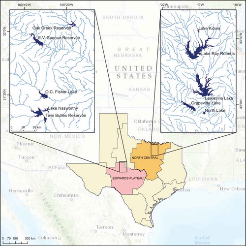
The aim of this study is to identify and investigate the spatial and the temporal patterns of change in the surface water area of 10 selected lakes in Texas, as well as assess the factors that might have impacted them during the 2005–2016 period. Five reservoirs near San Angelo and five reservoirs near Dallas (Figure 1) have been studied in both summer and winter months to explore the impact of drought and to compare how the drought has affected different regions in Texas between 2005 and 2016.

Figure 1. Location map for the selected lakes in San Angelo and Dallas. The Edwards Plateau Climate Division (marked with light red color) encompasses all lakes in the San Angelo study area, and the North Central Climate Division (indicated with light orange color) comprises the Dallas area lakes. All other climate divisions in Texas are marked with pale yellow color.

Landsat images have been used broadly in previous studies to identify changes in surface water bodies (e.g., Gilmer and Work 1975; White 1978; Rundquist et al. 1987; Li, Wang, and Duan 2015; Kaplan and Avdan 2017; Hossen et al. 2018; Policelli et al. 2018). There are also numerous publications on the advances in remote sensing and Geographic Information Systems (GIS) to monitor drought and assess its impact (e.g., Rhee, Im, and Carbone 2010; AghaKouchak et al. 2015; Thenkabail and Rhee 2017). In this study, we have adapted an effective density slicing approach that is capable of extracting the desired geospatial details from an individual Landsat band using Jenks natural breaks algorithm. Such an approach has allowed us to accurately estimate, characterize, and compare changes in the surface water area in both space and time, as indicated by the statistical analysis of the results. Our new results and interpretations provided in this study can enhance the water resource management in Texas and can support the policy maker with essential details to make informed decisions. This paper is derived from a master thesis by the first author (Asbury 2018), which is supported by more examples from California.

2. Study areas

San Angelo, located in west central Texas, has a total of 8 large lakes within 100 km of its city center. The lakes have a total surface area of 173.1 km² and 692.3 km of shoreline (Dowell 1964). We have selected 5 major lakes in San Angelo, located in Coke County in the north and Tom Green County in the south, to include in this study (Figure 1). The land cover in this study area is predominantly scrubland. Increasing urban and business development within the study area is a possible contributing factor to the current status of the surface water reservoirs (NLCD 2016).

Dallas, located in northeast Texas, has 3 reservoirs within 10 km of its city limits and two others less than 30 km away. These 5 reservoirs have a total surface area of 252.4 km² and 922.2 km of shoreline. The reservoirs are mainly located in Denton County and partially fall into four bordering counties, which include Crooke, Grayson, Tarrant, and Dallas Counties (Dowell 1964). The main land use in this study area is urban and business development and is surrounded by the major metropolitan area of Dallas and Fort Worth (NLCD 2016). Figure 1 shows the location of the 5 reservoirs as well as their proximity to Dallas.

3. Datasets and methods

Landsat-5, -7, and -8 scenes from 2005 through 2016 were obtained from the Earth Resources Observation and Science (EROS) data center operated by the United States Geological Survey (USGS). A total of 48 images were used, 24 images per location (12 acquisitions in winter plus 12 in summer). For the 2005–2012 period, Landsat-5 images were used when possible instead of Landsat-7 because of the radiometric striping that occurred in Landsat-7 images starting 2003 due to the failure of the Scan Line Corrector (SLC). Landsat-7 images were still used in some circumstances due to the presence of a dense cloud cover in Landsat-5 images or because they were the only available images from November 2011 through April 2013 for the selected lakes.

For San Angelo reservoirs, all Landsat scenes were selected with the least cloud cover possible from the Worldwide Reference System 2, path 29 and row 38. In the summer months, Landsat-5 images were used for 2005–2011, Landsat-7 images were used for only 2012, and Landsat-8 images were used for 2013–2016. In the winter months, Landsat-5 images were used for 2006–2011, Landsat-7 images were used for 2005, 2012, and 2013. Landsat-8 images were used for 2014–2016.

For Dallas reservoirs, all images were selected with the least cloud cover possible as well from the Worldwide Reference System 2, path 27 and row 37. In the summer months, Landsat-5 images were used for 2005–2007 and 2009–2011. Landsat-7 images were used for 2008 and 2012. Landsat-8 images were used for 2013–2016. In the winter months, Landsat-5 images were used for 2005 and 2007–2010. Landsat-7 images were used for 2006 and 2011–2013. Landsat-8 images were used for 2014–2016.

All Landsat images used in this study were geometrically and radiometrically corrected by USGS. Collection-1 – Higher Level (On-Demand) images that we obtained were processed for surface reflectance, top of atmosphere, brightness temperature, and spectral indices (Young et al. 2017). These corrections are necessary for any time-series analysis of satellite images; otherwise, images cannot be compared correctly to each other. The corrected satellite images were then formatted as GeoTIFF and projected into the Universal Transverse Mercator (UTM), World Geodetic System 1984 (WGS84), Zone 14N. When Landsat-7 images with stripes were used, the missing pixel values were retrieved using the average from the 5 nearest pixels. This simple interpolation was adequate for the purpose of our analysis since we are interested in studying only the water bodies. Water has nearly no reflectance in the NIR region, thus band-4 from Landsat-5 and -7 and its equivalent band-5 from Landsat-8 images were used to delineate water/land boundaries for the 10 selected lakes. The raster images from the near infrared (NIR) bands for each lake were classified using the lake boundary (the conservation pool top obtained from NLCD, 2016) as a mask to slice the surface area of each lake into three main categories according to the natural breaks inherent in the Landsat images.

The density slicing approach with the underlying Jenks natural break optimization method were employed to slice the raster NIR bands for all reservoirs into three desired categories (i.e., deep water, shallow water, and dry area). Density slicing is a technique of one-dimensional classification in which the continuous grey scale of an individual image band is sliced into a series of classes based on ranges of brightness values. The natural break method divides the output raster into the needed number of zones, with the areas of each zone determined by the class break. In this method, the classes are determined based on natural grouping that is inherent in the raster data. The break points are identified by choosing the class breaks that best group similar values and that create the maximum distance between classes, the cell values are divided into the corresponding zone when the borders have reasonably big jumps in the data values (Esri 2017). In this study, we used the ArcGIS suite developed by Esri (2017) to conduct the density slicing, but the analysis could be conducted by almost all available software packages for digital image processing and geospatial analysis.

The Jenks natural breaks algorithm, sometimes referred to as the Jenks optimization method (Coulson 2006), operates a multi-iteration process that is repeated until the set of breaks in the data has the smallest variance between classes. The process starts by dividing the individual reservoir into groups. The initial divisions can be arbitrary and these four steps are repeated: (1) calculate the sum of squared deviations between classes (SDBC), (2) calculate the sum of squared deviations from the array mean (SDAM), (3) subtract SDBC from SDAM (this equals the sum of squared deviations from the class means (SDCM)), and (4) inspect SDBC and a decision is made to move one unit from the class with the largest SDBC toward the class with the lowest SDBC (Jenks 1967). New class divisions are then calculated and the process is repeated until the sum of the class deviations reaches a minimal value. Finally, the features are divided into groups inherent to the data (Longley et al. 2015). The Goodness of Variance Fit (GVF) is used as a decision tool with a range of values from 0 to 1 (0 being the worst fit and 1 is the best fit). GVF can be simply expressed as in Equation 1 and can be computed as in Equation 2.

(1) $GVF=\frac{SDAM-CM}{SDAM},$(1)

Where SDAM is the sum of squared deviations from the array mean and SDCM is the sum of squared deviations from the class means.

(2) $GVF=1-\frac{\sum _{j=1}^k\sum _{i=1}^{N_j}{\left(z_{ij-{\bar{Z}}_J}\right)}^2}{{\sum }_{i=1}^N{\left(z_i-\bar{z}\right)}^2},$(2)

Where k is the number of desired classes (3 in our case: deep water, shallow water, and dry area), N is the set of values in class j, Z belongs to the value in class j, and $\bar{Z}$ is the mean value from class j.

Alternative methods of slicing the reservoirs into distinct areas include equal area and equal interval. When the equal area method is applied, the sliced output will have the desired number of zones with a similar number of pixels in each area. The equal interval method divides the raster image into the desired number of zones with each area containing an equal value range (Dent 1999). However, these two latter methods were not adapted in this investigation because they are not ideal for the nature of the desired geospatial analysis.

The accuracy assessment is a necessary step of any image classification (Lunetta and Lyon 2004) and we accomplished it by comparing the classified product to a verified reference at selected sample locations on a pixel-by-pixel basis. Results presented in Tables 1 and 2 show the accuracy assessment of the classified images for each reservoir, with an overall accuracy of approximately 94%, based on 100 random samples of pure pixels selected from each category per lake to assess the accuracy of the classified outputs. These samples were compared to independent measurements from the radiometrically and geometrically corrected Advanced Spaceborne Thermal Emission and Reflection Radiometer images, and all the classified products that showed inadequate accuracies were reprocessed to achieve a minimum of 90% accuracy.

Table 1. Statistical results of the accuracy assessment (%) for the selected reservoirs in San Angelo.

Year	Season	E.V. Spence	O.C. Fisher	Oak Creek	Twin Buttes	Nasworthy
2005	Winter	94	96	97	91	99
	Summer	91	95	92	96	99
2006	Winter	91	93	91	93	95
	Summer	99	96	96	92	91
2007	Winter	94	90	96	93	92
	Summer	93	93	96	96	99
2008	Winter	99	98	91	97	97
	Summer	90	97	91	92	95
2009	Winter	98	92	93	97	97
	Summer	92	94	92	90	98
2010	Winter	93	92	99	91	97
	Summer	90	97	91	93	94
2011	Winter	91	98	93	94	99
	Summer	92	97	95	94	99
2012	Winter	91	98	91	98	98
	Summer	90	97	94	91	99
2013	Winter	91	97	93	95	94
	Summer	93	91	95	99	96
2014	Winter	93	95	99	93	98
	Summer	93	90	95	94	91
2015	Winter	99	91	99	98	95
	Summer	90	92	93	90	99
2016	Winter	91	98	93	92	90
	Summer	96	95	97	91	92

Table 2. Statistical results of the accuracy assessment (%) for the selected reservoirs in Dallas.

Year	Season	Ray Roberts	Lewisville	Grapevine	Kiowa	North
2005	Winter	97	93	92	98	97
	Summer	94	93	96	98	95
2006	Winter	90	96	92	94	91
	Summer	90	92	91	95	92
2007	Winter	98	93	93	91	94
	Summer	98	95	94	90	92
2008	Winter	95	91	91	96	93
	Summer	99	99	94	90	94
2009	Winter	98	91	99	99	97
	Summer	92	96	92	99	90
2010	Winter	90	93	90	99	91
	Summer	90	91	95	99	90
2011	Winter	90	99	98	98	92
	Summer	93	94	96	99	97
2012	Winter	95	98	93	92	93
	Summer	91	93	93	90	91
2013	Winter	90	91	97	92	99
	Summer	93	91	97	99	93
2014	Winter	92	90	98	99	99
	Summer	99	94	94	92	93
2015	Winter	90	91	93	91	96
	Summer	98	95	90	90	97
2016	Winter	97	95	96	93	91
	Summer	95	96	95	92	97

There are several methods available for measuring and quantifying drought. In this study, three of Palmer’s drought indices were used including Palmer Z-Index, Palmer Drought Severity Index (PDSI), and Palmer Drought Hydrological Index (PDHI). The raw climate data used in this study were obtained from NOAA. Palmer’s drought indices use estimations of precipitation, temperature, and soil water content. The normal range of values extend from −4, which is very dry, to +4, which is extremely wet. Yet, values of −1 still indicate some level of drought as the values decrease and become more negative with a rise in temperature and a decrease in rainfall. These indices are very helpful in diagnosing agricultural drought due to its sensitivity to the soil conditions; however, they do not take into account stream flows (Vose et al. 2014). The Palmer Z-Index demonstrates how monthly moisture conditions depart from the average (i.e., it measures drought on a monthly scale), thus it is best suited for studying short-term drought. It is commonly used for measuring moisture changes over periods that last less than 12 months (Linsley, Kohler, and Paulhus 1975). PDSI measures long-term meteorological drought and wet conditions. It takes a cumulative measurement of many of the previous month’s weather patterns, with the current month being weighed more heavily. Weather may change rapidly, and therefore PDSI can respond quickly (Davitaya 1962). PDHI uses similar measurements to PDSI, but it reflects more accurately groundwater conditions and reservoir levels; consequently, PDHI responds slower than PDSI (Davitaya 1962).

4. Results and discussions

4.1. Surface water area oscillations

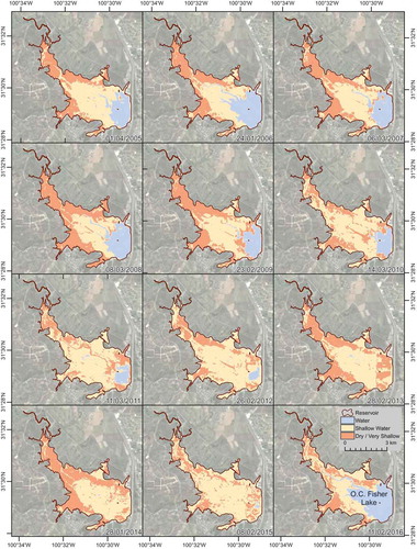
Five lakes in the San Angelo area; namely, Oak Creek, E.V. Spence, Nasworthy, Twin Buttes, and O.C. Fisher, were monitored throughout the study period (2005–2016). A detailed time series of surface water area change was created for each reservoir from both winter and summer acquisitions, but due to space considerations we provide only the quantifiable measurements from the winter time series of O.C. Fisher Lake (Figure 2) as a representation for the San Angelo area. However, Table 3 summarizes surface water area changes in the five studied reservoirs. Results indicate that all reservoirs in San Angelo were very drastically affected during 2005–2016. For instance, the surface water area of Oak Creek reservoir was reduced from 88% to 21% between 2008 and 2014. Likewise, the E.V. Spence reservoir lost nearly 88% of its original surface area just between 2008 and 2012. It is noteworthy that Lake Nasworthy experienced minimal oscillations and was kept at a constant level by gaining water from the Twin Buttes reservoir; meanwhile, the Twin Buttes reservoir dropped from 50% full to approximately 5%, with a considerable part of that was due to the discharge of water into the neighboring Lake Nasworthy. Surprisingly, the O.C. Fisher Lake nearly dried up by 2014 showing <1% of the possible surface area still made up of water in the reservoir, with nearly a 100% loss between 2006 and 2014 (Figure 2).

Table 3. Seasonal oscillations (%) in the surface water area of the selected reservoirs in San Angelo. The percentage of surface water area change is calculated with respect to the total possible surface area prescribed by the Texas Water Development Board.

Year	Season	Oak Creek	E.V. Spence	Nasworthy	Twin Buttes	O.C. Fisher
2005	Winter	28.8	58.8	82.1	30.2	15.9
	Summer	33.3	60.6	76.7	33.2	24.6
2006	Winter	35.9	64.5	75.8	37.3	24.9
	Summer	30.5	57.4	77.5	30.9	19.9
2007	Winter	22.1	55.2	79.7	33.3	17.1
	Summer	88.5	61.9	80.4	43.7	22.7
2008	Winter	88.3	56.8	76.5	49.4	19.6
	Summer	81.9	53.4	74.2	39.2	15.2
2009	Winter	79.4	47.5	77.0	38.0	12.8
	Summer	73.3	37.8	73.8	33.6	11.1
2010	Winter	70.7	29.7	80.1	34.4	10.4
	Summer	70.7	28.1	74.6	30.0	8.2
2011	Winter	68.5	24.4	79.5	27.9	6.0
	Summer	56.6	13.4	78.6	16.9	1.3
2012	Winter	48.3	9.0	85.4	15.3	2.4
	Summer	41.1	9.0	78.7	12.4	0.1
2013	Winter	38.4	33.4	82.4	15.0	0.2
	Summer	34.0	31.7	78.5	5.3	0.6
2014	Winter	21.0	26.9	76.8	8.4	0.1
	Summer	28.2	19.5	80.0	18.4	5.4
2015	Winter	25.0	24.6	80.3	16.9	0.4
	Summer	41.7	40.2	81.4	21.6	26.2
2016	Winter	46.0	48.2	80.7	18.6	32.5
	Summer	59.4	49.2	79.6	24.1	30.1

Figure 2. Surface water area oscillations in the O.C. Fisher Lake from winter acquisitions of each year during the study period (2005–2016). Dates are dd/mm/yyyy and the image from 2015 is used in the background because it has 0% cloud cover.

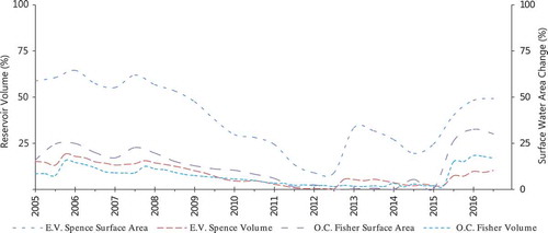
The surface water area change measured from satellite images does not always correlate closely with the volume change of a reservoir. Steep sides of a reservoir may result in a situation with minimal surface water area change but incredible volume change; while the opposite is true about reservoirs with very shallow-dipping sides. For instance, field measurements indicate that the E.V. Spence Lake is at 65% of its surface area coverage when it is about 20% full. Similarly, O.C. Fisher Lake reaches 30% of its surface water area coverage when it is at 18% of its total volume (Figure 3). Volume change measurements were obtained from TWDB. Estimating volume change from satellite images would require an accurate determination of the water depth via bathymetric data for each reservoir, which unfortunately are unavailable for our selected lakes. A traditional Digital Elevation Model (DEM) would not be helpful with that regard.

Figure 3. A comparison of oscillations in the surface water area and the volume of the E.V. Spence and the O.C. Fisher Lakes between 2005 and 2016.

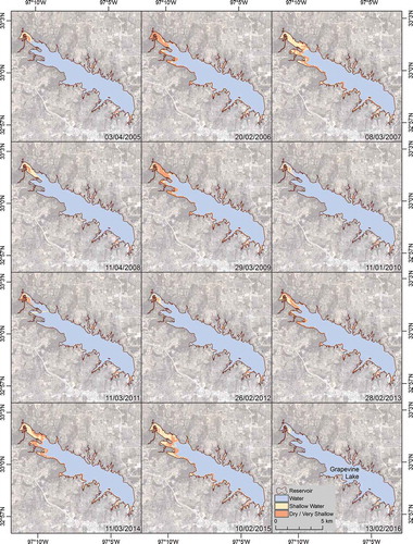
Five more lakes were studied in Dallas, including Grapevine, Ray Roberts, Lewisville, Kiowa, and North Lakes. Figure 4 shows the time series for the Grapevine Lake, which has been chosen to represent the Dallas study area because of the availability of its evaporation and discharge data. Table 4 shows changes in the surface water area of the five studied reservoirs in Dallas. Each one of the first three lakes; namely Grapevine, Ray Roberts, and Lewisville, is more than 10 times the surface area of Kiowa and North Lakes. Lake Ray Roberts lost nearly 30% of its surface area and Lewisville Lake experienced about 40% decrease of its surface coverage between 2005 and 2016. The largest three reservoirs (Grapevine, Ray Roberts, and Lewisville) reached their smallest surface areas during the winter of 2006 and the summer of 2014. There are not enough publicly available details regarding Kiowa and North Lakes probably because both of them are very small and Lake Kiowa is centered in a private community. North Lake appears to have been in the process of being drained based on our recent Landsat observations.

Table 4. Seasonal changes (%) in the surface water area of the selected reservoirs in Dallas during 2005–2016. The percentage of surface water area change is calculated with respect to the total possible surface area prescribed by the Texas Water Development Board.

Year	Season	Grapevine	Ray Roberts	Lewisville	Kiowa	North
2005	Winter	89.5	88.4	81.3	79.4	91.7
	Summer	85.3	93.6	84.8	86.1	93.3
2006	Winter	80.4	78.9	64.7	91.9	90.5
	Summer	74.3	84.1	71.6	84.8	84.6
2007	Winter	72.4	80.7	82.5	87.8	84.0
	Summer	94.8	96.1	94.4	71.1	65.3
2008	Winter	91.7	85.9	76.9	74.1	91.8
	Summer	83.6	95.0	88.4	82.9	88.6
2009	Winter	78.5	91.5	83.1	85.0	88.9
	Summer	86.7	95.4	92.2	84.1	83.9
2010	Winter	91.4	95.5	93.8	81.6	77.5
	Summer	90.7	94.4	90.2	82.3	77.0
2011	Winter	83.0	92.4	87.6	78.0	71.8
	Summer	88.4	90.1	83.9	85.8	73.0
2012	Winter	89.7	82.3	76.3	77.3	68.0
	Summer	87.3	94.5	88.9	84.0	72.9
2013	Winter	81.8	88.6	78.8	84.8	68.4
	Summer	78.7	86.0	78.8	88.6	68.3
2014	Winter	75.9	81.2	77.2	88.7	67.0
	Summer	76.3	79.1	78.3	88.8	24.5
2015	Winter	72.3	80.7	78.6	87.8	21.7
	Summer	97.8	98.0	97.1	83.7	29.6
2016	Winter	97.9	98.1	94.8	83.5	30.1
	Summer	93.5	96.2	93.6	83.8	28.7

Figure 4. Surface water area changes in the Grapevine Lake from winter acquisitions of each year during 2005–2016. Dates are dd/mm/yyyy and the image from 2015 is used in the background because it has no cloud cover.

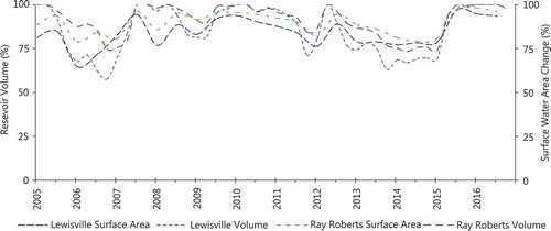
Landsat observations and field measurements in Dallas indicate that when the surface water area increased slightly, the lake volume increased more rapidly. For example, when Lake Ray Roberts was at 100% volume, the surface water area reached only 90–95% coverage. Also, Lewisville Lake covered about 85% of its surface area when its volume was at 100% capacity as shown in Figure 5. Volume change measurements were obtained from TWDB.

Figure 5. A comparison of oscillations in the surface water area and the volume of the Lewisville and the Ray Roberts Lakes.

4.2. Impact of climate

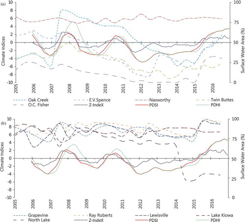
Climate divisions in the United States were essentially developed to generate historical climate data. They were developed to monitor drought, temperature, and precipitation at local, state, regional, and nationwide levels (Wilhite and Glantz 1985). The local climate conditions were the same for all lakes in San Angelo, and most of the reservoirs followed the climate conditions during the study period but with varying magnitudes. The Oak Creek reservoir experienced a considerable reduction of about 67% of its surface water area between 2008 and 2014. The climate conditions were generally dry during that time period and the climate indices reached above zero only in 2 out of the 6 years. With the wet conditions prevailing in 2015, the surface water area had nearly doubled in size (Table 3, Figure 3). The E.V. Spence reservoir decreased considerably from nearly 65% in 2006 to less than 10% in 2014. The reservoir had a slight increase to 30% over the next year followed by a sharp decrease and the surface water area was in excess of its double (Table 3, Figure 3). The same climate conditions were experienced with different outcomes, leading to the thought that other non-climate factors affected the lake levels. Lake Nasworthy showed slight to no correlation with climate conditions, but that is expected since it was kept at a constant level from the neighboring Twin Buttes Lake that lost approximately 45% of its surface area between 2008 and 2013 (Table 3, Figure 3). O.C. Fisher Lake dried up for nearly four years and decreased in size from 25% in 2005 to 0% between 2012 and 2015. With the dramatic change to wet conditions in early 2015, this reservoir recovered nearly 30% of its surface area (Table 3, Figure 3).

A visual comparison of Figure 6 (a) and (b) shows that the five reservoirs studied in Dallas appear to not change as drastically as those reservoirs in San Angelo. Dallas area experienced similar periods of dry and wet conditions; however, the levels of dryness were more severe in the Edwards Plateau climate division and the periods of wetness were greater, as observed from the climate indices of the North Central climate division. Grapevine Lake decreased from 90% to 72% during the dry climate period, and then rebounded to 98% of its surface area in 2016 (Table 4, Figure 5). Lake Ray Roberts is the largest of the five studied reservoirs. Similar to Grapevine and Lewisville Lakes, it experienced comparable expansion and contraction periods. The peak of its surface area was at 94% in 2007, then decreased to 79% by 2014 (Table 4, Figure 5). Lake Lewisville followed a similar change pattern, as shown in Figure 6. It reached its minimum surface area in 2014 toward the end of the dry period, then expanded to 97% in 2015. Lake Kiowa is a much smaller reservoir that showed a dissimilar reaction to climate conditions. Its surface water area remained 75%-85% covered during the entire study period, and the change pattern did not appear to correlate with any climate indices (Table 4, Figure 5). North Lake is also a very small lake that showed a gradual decrease until 2014 when a drastic decrease dropped its surface area percentage from 67% in 2014 to 25% in 2015 (Table 4, Figure 5). Apparently, this is due to constructional activities on the lake that is being drained, as seen from the time series of satellite images.

Figure 6. (a) Palmer drought indices for the Edwards Plateau climate division (marked with light red color in Figure 1) and surface water area changes in the San Angelo lakes. (b) Palmer drought indices for the North Central Texas division (marked with light orange color in Figure 1) and surface water area changes in the Dallas reservoirs.

4.3. Impact of evaporation and discharge

Undoubtedly, climate has a broad impact on the 10 studied lakes, but it is not the only factor causing changes in the surface water area of the reservoirs in Texas. The mean yearly evaporation rates are nearly twice the mean yearly precipitation rates along the Colorado River Basin that encompasses all the reservoirs studied in the San Angelo proximity. In the Trinity River Basin, which encapsulates the Dallas area reservoirs, the evaporation rates are nearly equivalent to the mean precipitation rates (Wurbs and Ayala 2014). The evaporation is measured daily at Grapevine and O.C. Fisher Lakes (Figure 7a). Discharge from reservoirs, with an instantaneous cubic foot per second (CFS), is measured hourly at Grapevine, Lewisville, Ray Roberts, and O.C. Fisher Lakes. Certainly, there are substantial discharge and evaporation from all other reservoirs, but unfortunately their records are not kept.

Figure 7. (a) The relationship between the surface water area and the average of evaporation recorded on site daily at the Grapevine and the O.C. Fisher Lakes by the Corps of Engineers and the Texas Water Development Board, respectively. (b) The relationship between changes in the surface water area and the average of daily discharge (the total m³/day) measured at the Grapevine and the O.C. Fisher Lakes by the Corps of Engineers and the Texas Water Development Board, respectively.

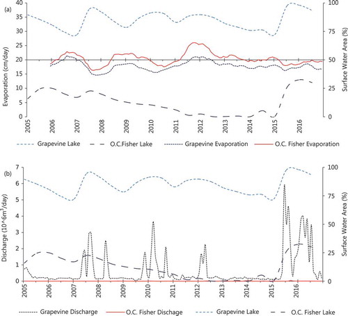
Discharge and evaporation data used in this study were obtained from TWDB and the Corps of Engineers. Figure 7b displays the recorded discharge at both lakes. The major spikes in the discharge levels at Grapevine Lake occurred while the lake was at its peaks; however, the discharge levels were barely noticeable at O.C. Fisher Lake. The figure also displays the average evaporation levels at each reservoir. It is obvious that O.C. Fisher Lake had slightly higher evaporation levels consistently throughout the study period (2005–2016). Increases in the evaporation level at both reservoirs correlated well with the shrinkage patterns of the surface water area, but changes in O.C. Fisher Lake were negligible at times when the lake was <1% covered.

5. Conclusions

Ten surface water reservoirs in Texas were studied in this geospatial investigation using Landsat images acquired between 2005 and 2016. Based on our results, we can conclude that: (1) the developed procedure using the density slicing is an efficient approach capable of expanding the geospatial details that can be extracted from a single Landsat band and thus can be adapted to study other lakes across the world, (2) all reservoirs in the San Angelo area are more noticeably affected by climate and human interference, (3) the Dallas reservoirs are correlating more closely to the drought indices during the study period, and (4) drought has played the major role in the expansion and shrinkage of the surface water area of all studied reservoirs, but other factors have had an impact as well.

Both study areas have experienced similar climate conditions with comparable wet and dry periods; however, the San Angelo study area has witnessed more drastic dry periods and the Dallas area has experienced more severe wet periods. Our results imply that drought conditions have had a substantial impact on the reservoirs in Dallas, as indicated by the high correlation with the local drought indices. For example, Grapevine Lake lost 18% of its surface area during the dry climate period and rebounded to 98% of its surface area in the rainy year of 2016. Meanwhile, the reservoirs in San Angelo are more greatly affected by more severe climate conditions, as shown by the extreme changes in surface water area, but with a weaker correlation to the local drought conditions. For instance, O.C. Fisher Lake decreased in size from 25% in 2005 to 0% during 2012–2015. The lake dried up fully for about four years continuously. It is also noticeable that human activity has played a considerable role in the changes in the surface water area of Twin Buttes and Nasworthy and most likely have contributed to changes in the other lakes as well. The obtained results will broaden understanding of the factors that have contributed to the intensive lake changes occurred in Texas during the study period and can definitely empower management of the water resources and can facilitate making relevant policies.

Acknowledgements

All Landsat images, raw climate data, and evaporation/discharge data are obtained from USGS, NOAA, and the Corp of Engineers/TWDB, respectively, at no cost. Thanks to Hafid Nanis, from the InSAR Research Group at the University of Arkansas, for his valuable discussion on climate data. Thanks are due also to Ralph Davis and David Stahle from the Department of Geosciences for the fruitful discussion of the results. This research has been accomplished using the InSAR Lab facility at the University of Arkansas. Finally, the authors would like to thanks the editor and the anonymous reviewers for their thorough reviews that substantially improved the quality of this publication.

Disclosure statement

No potential conflict of interest was reported by the authors.

References

- AghaKouchak, A., A. Farahmand, F. S. Melton, J. Teixeira, M. C. Anderson, B. D. Wardlow, and C. R. Hain. 2015. “Remote Sensing of Drought: Progress, Challenges and Opportunities.” Reviews of Geophysics 53: 452–480. doi:10.1002/2014RG000456.
- Anderson, D. P. 2014. “2010-2014 Texas Agriculture: The Economic Impact of Drought,” The National EDEN Annual Meetings, Florence, Alabama, 23 October 2014.
- Asbury, Z. 2018. “A Geospatial Study of the Drought Impact on Surface Water Reservoirs: Study Cases from Texas and California”. University of Arkansas, Theses and Dissertations, 2788. https://scholarworks.uark.edu/etd/2788
- Coulson, M. R. C. 2006. “In the Matter of Class Intervals for Choropleth Maps: With Particular Reference to the Work of George F Jenks.” Cartographica: the International Journal for Geographic Information and Geovisualization, October. doi:10.3138/U7X0-1836-5715-3546.
- Davitaya, F. F. 1962. “Agro-Meteorological Problems [Of the USSR]. Compendium of Abridged Reports to the Second Session of the Commission for Agricultural Meteo-Rology of the World Meteorological Organization.” Agro-meteorological problems [of the USSR]. https://www.cabdirect.org/cabdirect/abstract/19630700296
- Dent, B. D. 1999. Cartography-Thematic Map Design, 417. 5th ed. McGraw Hill. Boston, MA: William C Brown Pub.
- Dowell, C. L. 1964. Dams and Reservoirs in Texas: Historical and Descriptive Information. Austin, TX: Texas Water Commission.
- Esri, 2017. Accessed 24 April. http://resources.esri.com/help/9.3/ArcGISDesktop/com/Gp_ToolRef/spatial_analyst_tools/how_slice_works.htm
- Gilmer, D. S., and J. E. A. Work. 1975. “Utilization of Satellite Data for Inventorying Prairie Ponds and Lakes.” LANDSAT-1 Data Were Used to Discriminate Ponds and Lakes for Waterfowl Management. [Alaska, Canada, and Dakotas]. https://ntrs.nasa.gov/search.jsp?R=19760021508
- Hossen, H., M. G. Ibrahim, W. E. Mohmod, A. Negm, K. Nadaoka, and O. Saavedra. 2018. “Forecasting Future Changes in Manzala Lake Surface Area by considering Variations in Land Use and Land Cover Using Remote Sensing Approach.” Arabian Journal of Geosciences 11 (5): 1–17. doi:10.1007/s12517-018-3416-7.
- Jenks, G. F. 1967. “The Data Model Concept in Statistical Mapping.” International Yearbook of Cartography 7: 186–190.
- Kaplan, G., and U. Avdan. 2017. “Water Extraction Technique in Mountainous Areas from Satellite Images.” Journal of Applied Remote Sensing 11 (4): 046002. doi:10.1117/1.JRS.11.046002.
- Li, J., J. Wang, and P. Duan. 2015. “Remote Sensing Monitoring Study for Water Area Change of Fuxian Lake in Last 40 Years.” In International Conference on Intelligent Earth Observing and Applications 2015, 9808:980824.International Society for Optics and Photonics, Guilin, China. doi:10.1117/12.2210975.
- Linsley, R. K., M. A. Kohler, and J. L. H. Paulhus. 1975. Hydrology for Engineers, 482. 2nd ed. Kogukusha, Tokyo: McGraw Hill.
- Longley, P. A., M. F. Goodchild, D. J. Maguire, and D. W. Rhind. 2015. Geographic Information Science and Systems. Hoboken, NJ: John Wiley & Sons.
- Lunetta, R. S., and J. G. Lyon. 2004. Remote Sensing and GIS Accuracy Assessment, 326. Boca Raton, FL: CRC press.
- McPhaden, M. J. 1999. “Genesis and Evolution of the 1997-98 El Niño.” Science 283 (5404): 950–954. doi:10.1126/science.283.5404.950.
- McPhaden, M. J., S. E. Zebiak, and M. H. Glantz. 2006. “ENSO as an Integrating Concept in Earth Science.” Science 314 (5806): 1740–1745. doi:10.1126/science.1132588.
- National Land Cover Database, 2016. “Texas Natural Resources Information System (TNRIS).” https://tnris.carto.com/viz/d5084e86-dec9-11e4-afda-0e0c41326911/embed_map
- Nielsen-Gammon, J. 2011. “The 2011 Texas Drought: A Briefing Packet for the Texas Legislature.” Technical report, Texas A&M Libraries, 43
- Policelli, F., A. Hubbard, H. Jung, B. Zaitchik, and C. Ichoku. 2018. “Lake Chad Total Surface Water Area as Derived from Land Surface Temperature and Radar Remote Sensing Data.” Remote Sensing 10 (2): 252. doi:10.3390/rs10020252.
- Rhee, J., J. Im, and G. J. Carbone. 2010. “Monitoring Agricultural Drought for Arid and Humid Regions Using Multi-Sensor Remote Sensing Data.” Remote Sensing of Environment. doi:10.1016/j.rse.2010.07.005.
- Rundquist, D. C., M. P. Lawson, L. P. Queen, and R. S. Cerveny. 1987. “The Relationship between Summer Season Rainfall Events and Lake Surface Area.” JAWRA Journal of the American Water Resources Association 23 (3): 493–508. doi:10.1111/j.1752-1688.1987.tb00828.x.
- South Central Climate Science Center. 2013a. “Drought History for North Central Texas.” Accessed 18 August 2017. http://www.southcentralclimate.org/index.php
- South Central Climate Science Center. 2013b. “Drought History for the Edwards Plateau of Texas.” Accessed 18 August 2017 . http://www.southcentralclimate.org/index.php
- Texas Water Development Board (TWDB). 2017. Accessed 23 November 2017 http://www.twdb.texas.gov/mapping/gisdata.asp
- Thenkabail, P. S., and J. Rhee. 2017. “GIScience and Remote Sensing (TGRS) Special Issue on Advances in Remote Sensing and GIS-based Drought Monitoring.” GIScience & Remote Sensing 54 (2): 141–143. doi:10.1080/15481603.2017.1296219.
- Vose, R. S., S. Applequist, M. Squires, M. J. Imke Durre, C. N. Menne, C. F. Williams, K. Gleason, and D. Arndt. 2014. “Improved Historical Temperature and Precipitation Time Series for U.S. Climate Divisions.” Journal of Applied Meteorology and Climatology 53 (5): 1232–1251. doi:10.1175/JAMC-D-13-0248.1.
- White, M. E. 1978. “Reservoir Surface Area from Landsat Imagery [Development of Urban and Agricultural Water Supplies, New Mexico].” Photogrammetric Engineering and Remote Sensing. http://agris.fao.org/agris-search/search.do?recordID=US19790406004
- Wilhite, D. A., and M. H. Glantz. 1985. “Understanding: The Drought Phenomenon: The Role of Definitions.” Water International 10 (3): 111–120. doi:10.1080/02508068508686328.
- Wurbs, R. A., and R. A. Ayala. 2014. “Reservoir Evaporation in Texas, USA.” Journal of Hydrology 510: 9. doi:10.1016/j.jhydrol.2013.12.011.
- Young, N. E., R. S. Anderson, S. M. Chignell, A. G. Vorster, R. Lawrence, and P. H. Evangelista. 2017. “A Survival Guide to Landsat Preprocessing.” Ecology 98: 920–932. doi:10.1002/ecy.1730.