Landslide susceptibility mapping by remote sensing and geomorphological data: case studies on the Sorrentina Peninsula (Southern Italy)

Abstract

The Sorrentina Peninsula is a densely populated area with high touristic impact. It is located in a morphologically complex zone of Southern Italy frequently affected by dangerous and calamitous landslides. This work contributes to the prevention of such natural disasters by applying a GIS-based interdisciplinary approach aimed to map the areas more potentially prone to trigger slope instability phenomena. We have developed the Landslide Susceptibility Index (LSI) combining five weighted and ranked susceptibility parameters on a GIS platform. These parameters are recognized in the literature as the main predisposing factors for triggering landslides. This work combines analyses conducted on Remote Sensing, Geo-Lithology and Morphometry data and it is organized in the following logical steps: i) Multi-temporal InSAR technique was applied to Envisat-ASAR (2003–2010) and COSMO-SkyMed (2013–2015) datasets to obtain the ground displacement time series and the relative mean ground velocity maps. InSAR allowed the detection of the areas that are subjected to ground deformation and the main affected municipalities; ii) Such deformation areas were investigated through airborne photo interpretation to identify the presence of geomorphological peculiarities connected to potential slope instability. Subsequently, some of these peculiarities were checked on the field; iii) In these deformation areas the susceptibility parameters were mapped in the entire territory of Amalfi and Conca dei Marini and then investigated with a multivariate analysis to derive the classes and the respective weights used in the LSI calculation. The resulting LSI map classifies the two municipalities with high spatial resolution (2m) according to five classes of instability. The map highlights that the high/very high susceptibility zones cover 6% of the investigated territory and correspond to potential landslide source areas characterized by 25°-70° slope angles. A spatial analysis between the map of the historical landslides and the areas classified according to susceptibility allowed testing of the reliability of the LSI Index, resulting in 85% prediction accuracy.

Keywords:

• landslide
• remote sensing
• GIS-based
• susceptibility index
• Sorrentina Peninsula

1. Introduction

The Sorrentina Peninsula is located in Southern Italy (Campania Region) between Salerno and Naples Gulfs. Covering an area of 197 km² the peninsula constitutes the final termination of the NE-SW trending Lattari Mountains carbonatic ridge, perpendicular to the Apennines chain (Figure 1). The Peninsula includes 21 municipalities, 18 along the coast and 3 inland, and represents one of the more densely populated areas in the Campania region, with a high tourism impact, in particular along the coastal localities. During the last 1000 years, hundreds of disastrous terrain instability and flooding events have affected the Peninsula, also involving human settlements located at the base of slopes and/or inside valleys (Porfido et al. 2009). These events, often catastrophic, caused fatalities and heavy damage to infrastructures, private property and road networks. In chronological order, the first documented event was the “Cappuccini landslide,” a rock fall with a volume of about 2 × 10⁴ m³, that affected the Amalfi town on 21 December 1899. In October 25–26, 1954, heavy flood and landslides affected many coastal villages between Salerno and Ravello causing disastrous consequences: 316 casualties; 320 buildings were completely destroyed and 279 damaged; the road network was interrupted for days; and 10,064 people became homeless (Esposito, Porfido, and Violante 2004). This event was triggered by strong rain that hit several localities simultaneously, particularly in Salerno town where 500 mm of rain fell in 16 hours reaching a peak of 150 mm/h (Esposito, Porfido, and Violante 2004). Finally, on January 9–11, 1997, a volcanoclastic debris flow affected Pozzano village causing 4 fatalities, injuring 22 persons and interrupting the main coastal road for about 2 months. This event was preceded by intense rainfall that reached a total of 160 mm in 48 hours (Calcaterra and Santo 2004).

Figure 1. Sorrentina Peninsula Geological map (modified after Apuzzo et al. 2013).

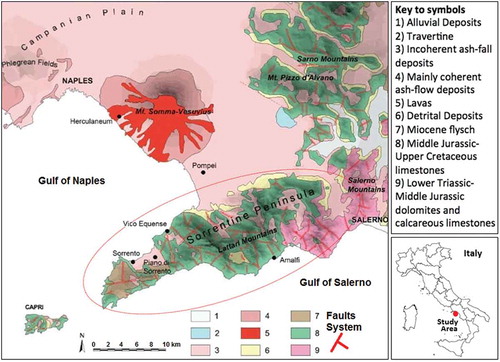
The large number and variety of landslides recorded in the Peninsula are mainly due to the peculiar geomorphology and lithology of the area where the calcareous bedrock of very steep hillslopes, characterized by faults and fractures, is mantled by ash-fall deposits produced by the explosive activity of Mt. Somma-Vesuvius complex and Phlegrean Fields over last 40 k.y. (Calcaterra, Parise, and Palma 2003; Cioni et al. 2003; Budetta, De Riso, and Santo 2005).

The historical landslides occurred in the Peninsula in the last 1000 years have been collected by the Regional Basin Authorities into a database (http://adbcampaniasud.it/web/pianificazione/documenti-generali) updating at 1:5000 scale two existing catalogues PSAI (Piano Stralcio di Bacino per l’Assetto Idrogeologico) and IFFI (Inventario dei Fenomeni Franosi in Italia). The PSAI catalogue includes 3253 landslides at regional scale and is based on geomorphological data. The IFFI catalogue contains more than 460,000 landslides all over Italy, in particular 4255 in Sorrentina Peninsula (Trigilia and Iadanza 2007).

Most of the previous studies aimed to map the areas that are potentially prone to slope instability, and were generally based on inventory of historical landslides (Guzzetti et al. 2012; Apuzzo et al. 2013; Luca’ et al., 2014). This work, instead, starts from the analysis of long sequences of Synthetic Aperture Radar (SAR) scenes to identify areas that are undergoing slow deformation (few mm/y). A GIS-based interdisciplinary approach has been applied by combining Geo-Lithology and Morphometry data with Remote Sensing analyses to map the source zones that are potentially prone to landslide triggering.

In the literature, the identification and measurement of ground deformations include Remote Sensing techniques (Metternicht, Hurni, and Gogu 2005; Jaboyedoff et al. 2012) such as Airborne/Satellite Photogrammetry, Airborne/Terrestrial Laser Scanning (Slob and Hack 2004) and SAR (Colesanti et al. 2003). In particular, Interferometric SAR techniques (InSAR/DInSAR) were applied to long temporal datasets to identify and measure with high accuracy (sub cm) the ground displacements investigating large and sparsely vegetated areas at reasonable cost (Massonnet et al. 1994; Singhroy and Molch 2004). Since 90ʹ years the InSAR technique has been developed to detect small ground deformations (Bürgmann et al., 2000). In fact, it is possible to detect very slow mass movements up to 16 mm/y if the displacement gradient between adjacent pixels in a SAR dataset is less than half the radar wavelength (Metternich et al., 2005). Such movements represent possible precursors to slope deformation that often precede landslides (Corsini et al. 2006). The European space missions of the Earth Resource Satellite (ERS-1/2) and ENVISAT SAR sensors, operating in C-band frequency, measure the long periods ground displacements. By quantifying such displacement it is possible to investigate the history evolution of slope deformation (Hopper, 2008; Bovenga et al. 2012). Most recently, with the advent of the new SAR systems, such as Sentinel-1 and X-band COSMO-SkyMed constellations with improved temporal sampling (Sentinel-1 up to 6 days) and high ground resolution (up to 1m in COSMO-SkyMed “Spot light” mode), it is possible to investigate the ground deformations with highly variable temporal trends (Bovenga et al. 2013; Calò et al. 2014; Herrera et al. 2013 Raspini et al. 2018). Thanks to the high ground resolution there is a significant increase in the number of the measurement points, improving SAR capability in terms of mapping and monitoring landslides (Calo’ et al. 2014, Bovenga et al. 2013, 2012; Cascini, Fornaro, and Peduto 2010; Colesanti and Wasowski 2006). In order to investigate slope instability on Peninsula Sorrentina, this work analyses the SAR C-band Envisat-ASAR and X-band COSMO-SkyMed datasets characterized by a displacement gradient less than 2.8 and 1.5 cm, respectively. These gradients, since they correspond to half wavelength of C and X bands radar pluses, are suitable for the detection of slow deformations that often characterize the time-period prior to landslides events (García-Davalillo et al. 2014). The use of both SAR bands maximizes the correlation level in vegetated areas and the number of measurement points. In detail, the deformations are identified and measured by a Multi-temporal InSAR technique. The radar images acquired at different times on the same region (i.e., repeat pass interferometry) are combined to obtain interferometric phases that, by measuring the radar-to-ground distance between image pairs, identify deformation that occurred in the time interval of the dataset in the satellite Line of Sight (LoS) direction (Bϋrgmann, Rosen, and Fielding 2000).

This work, aimed to map the Landslides Susceptibility, is organized in a series of logical steps. The workflow used in this study is illustrated in Figure 2 and starts with InSAR processing to identify areas that are subjected to ground deformation. In the second step, such areas are investigated by airborne photo-geological analysis and then checked on the field in order to find out morphological peculiarities connected to slope instability phenomena. In the third step a multivariate analysis is applied to the susceptibility parameters mapped in the checked deformation areas in order to derive the classes and the respective weights for each parameter in the LSI calculation. Finally, the LSI Susceptibility map and the relative accuracy are performed.

Figure 2. Methodological approach scheme.

2. InSAR: analyses and results

This section presents the InSAR processing: the dataset, visibility analysis, multi-temporal technique and the resulting deformation areas investigated in the subsequent steps indicated in the workflow of Figure 2.

2.1. SAR dataset

Two sets of SAR images have been processed in ascending and descending tracks (Table 1). The C-band ASAR dataset is composed of images with spatial resolution of 9 m (ground range) × 6 m (azimuth) acquired in the period 2003–2010 with a 35day revisit time. The X-band CSK dataset is composed of images with spatial resolution of 3 m (ground range) × 3 m (azimuth) acquired in the “StripMap” mode in the period 2013–2015 with a 16-day revisit time. Each image in the two datasets covers the entire Peninsula.

Table 1. Elaborated SAR dataset details.

Satellite	Track	Temporal interval	Images extent (Km)	Incidence Angle	Polarization	Images
ASAR Envisat	Ascending	13/11/02–16/12/09	100x100	23°	VV	48 scenes
ASAR Envisat	Descending	05/06/03–21/10/10	100x100	23°	VV	37 scenes
COSMO-SkyMed	Ascending	04/02/13–15/04/15	40x40	26.6°	HH	34 scenes
COSMO-SkyMed	Descending	03/03/12–19/12/13	40x40	32.2°	HH	29 scenes

2.2. InSAR visibility analysis

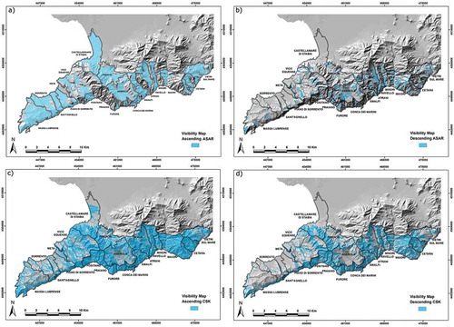
In the areas characterized by complex morphologies, such as the Sorrentina Peninsula, the radar image acquisitions can be limited by the view geometry. For this reason, before processing SAR data, “a priori” InSAR visibility maps (Cascini, Fornaro, and Peduto 2009) were generated to quantify the SAR areal coverage in each municipality. These maps are obtained by combining the ascending and descending tracks of Envisat-ASAR (ASAR) and COSMO-SkyMed (CSK) sensors with aspect and slope angles of the terrain, two factors that influence the SAR surface visibility (Table 2a, b). In the specific, the slope and aspect angles were derived from Shuttle Radar Topography Mission (SRTM-3 DEM) with cell size of 90 m (http://www2.jpl.nasa.gov/srtm). The ascending tracks of ASAR and CSK reveal the highest SAR visibilities covering 68% and 60% of the Peninsula, respectively (Figure 3). These percentages represent good visibility values taking into account the complex morphology of the Peninsula itself. On the other hand, the visibility of ASAR and CSK descending tracks are scarce covering only the 10% and 33% of Peninsula, respectively (Figure 3).

Table 2. SAR “a priori” visibility analysis: Terrain aspect and slope (SL) constraints for ASAR (a) and CSK (b) dataset.

ASAR (a)
Aspect	Ascending	Descending	Notes
E	SL<67° Enhanced range resolution SL>67° Shadow	SL<23° Foreshortening	SL>67° not covered
W	SL<23° Foreshortening	SL>23° Layover SL<67° Enhanced range resolution	SL>67° not covered
N/S	SL>23° Layover	SL>67° Shadow	Low system sensitivity to translational displacement along N/S
CSK (b)
Aspect	Ascending	Descending	Notes
E	SL<67° Enhanced range resolution SL>64° Shadow	SL<32° Foreshortening	SL>64° not covered
W	SL<26° Foreshortening	SL>32° Layover SL<64° Enhanced range resolution	SL>64° not covered
N/S	SL>26° Layover	SL>58° Shadow	Low system sensitivity to translational displacement along N/S

Figure 3. InSAR “a priori” visibility: a) ASAR ascending; b) ASAR descending; c) CSK ascending; d) CSK descending.

2.3. Multi-temporal InSAR analysis

The multi-temporal InSAR technique adopted in this study is the Small Baseline Subset (SBAS). It combines a large number of SAR differential interferograms characterized by short temporal and spatial orbital separations (baseline) in order to limit decorrelation effects and to maximize the number of coherent SAR targets detected on the ground (Berardino et al. 2002). Since this technique is able to identify isolated pixels surrounded by pixels that completely decorrelate (Hooper 2008; Cascini, Fornaro, and Peduto 2009), it is suitable to investigate the complex areas of Sorrentina Peninsula. The SBAS outputs are the ground displacements time series obtained through the inversion of the corrected interferometric phases and the mean ground velocity in the period covered by the dataset and calculated along the LoS direction. Conventionally, the velocity and the deformation are positive or negative when the radar pulse path length decreases or increases in LoS, respectively. The displacement time series and the mean ground velocity maps are affected by uncertainties due mainly to orbital errors, atmospheric heterogeneities, DEM and unwrapping errors (Casu, Manzo, and Lanari 2006). In particular, the influence of DEM errors on the ground velocities measured by SBAS is rather limited since the errors are iteratively estimated and removed during the processing. The estimation and removal of the atmospheric phase components includes a double-pass filtering in the temporal and spatial domains, considering that the atmospheric phase signal is highly correlated in space but poorly in time (Berardino et al. 2002). In order to improve the signal to noise ratio and the result quality, at the beginning of the processing, a multi-looking operation is performed to reduce the image radar noise and to define the output map cell size. The SBAS technique estimated error is ± 1mm/y on ground velocities and ±5 mm on ground displacements (Casu, Manzo, and Lanari 2006).

In this work, the SBAS technique has been performed using the SARScape software (Sarmap SA 5.2 version) for CSK data and Geohazards thematic Exploitation Platform for ASAR data (http://terradue.github.io/doc-tep-geohazards/). To produce the interferograms, we selected pairs of SAR acquisitions that satisfy the following conditions: (i) a spatial baseline (i.e., the perpendicular distance between the two tracks) <300 m for ASAR and <500 m for CSK; (ii) a temporal baseline (i.e., the separation in time between two images) of 1000 days for ASAR and 115 days for CSK. In detail, the ASAR dataset processing generated 182 and 177 interferograms for ascending and descending tracks, respectively. Whereas, the CSK dataset processing generated 77 and 91 interferograms for ascending and descending tracks, respectively. In the SBAS retrieval, the interferograms are coupled for maximizing the number of coherent pixels setting the most suitable output map cell size to preserve the coherence and investigate such phenomena (Berardino et al. 2002). The CSK mean multi-temporal coherence, obtained by combining the single interferogram spatial coherence maps, is 0.30 ± 0.13 and 0.38 ± 0.15 for ascending and descending tracks, respectively. At the end of the SBAS processing, the displacement time series are obtained and the respective mean ground velocity maps are produced without any spatial interpolation with a cell size of 40 m (ASAR) and 20 m (CSK).

2.4. InSAR results

The processing of ASAR and CSK ascending tracks identified ground deformations that cover 37% and 24%, respectively, of the entire Peninsula taking into account the “a priori” visibility. Figure 4a and 4b show the ASAR and CSK mean ground velocity maps derived from the respective displacement time series. The ASAR mean ground velocity map covers an area of 1.7 *10⁶ m² that, as expected, is greater than the CSK one (1.4 *10⁶ m²). This is due to the different time windows of the datasets and the incidence angle of the CSK X-band with respect to the ASAR C-band (Table 1).

Figure 4. InSAR processing results on the entire Peninsula: (a) ASAR mean ground velocities map; (b) CSK mean ground velocities map.

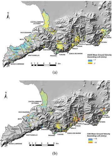
Both mean ground velocity maps highlight that the deformations affect mainly the coastal areas located between Conca dei Marini and Maiori municipalities (Figure 4a and 4b). In particular, calculating for each municipality the extent of ASAR and CSK areas in deformation (Table 3), Atrani, Amalfi and Conca dei Marini result the municipalities characterized by the highest percentage of total areas in deformation (90%, 32% and 23%), whereas the most significant velocity values affect the Amalfi and Conca dei Marini territory. Focusing on these two municipalities, the highest ground velocity areas are characterized by a large range of coherence (0.10–0.70). In order to detect the reliability of these areas we have investigated the highest coherence sites (>0.4). In detail, the ASAR map (Figure 5a) is characterized by a mean ground velocity ranging from −6 mm/y to −4 mm/y. We have analyzed (A), (B), (C) and (AMCH) points where the maximum displacement values are −58 mm and −55 mm (Figure 5b) recorded in (A) and (B) points, respectively located in Conca dei Marini bay (Figure 5c) and in the sector above Amalfi harbor (Figure 5d). The lowest value of −100 mm is referred to the (C) point located in the Agerola municipality slightly north of the Amalfi boundary (Figure 5c). In the CSK map, characterized by mean ground velocities ranging between −15 mm/y and −9 mm/y, we have analyzed the (D), (E), (F) and (AMCH) points (Figure 6a). The maximum value of displacement is −40 mm recorded in (E) point, whereas the (AMCH) point shows a displacement of −28 mm (Figure 6b). Both sites are located in Amalfi municipality. As regards ASAR and CSK descending tracks, the data processing does not reveal any deformation due to the poor visibility induced by the acquisition geometry and the complex topography of the area.

Table 3. Areal ground deformation coverage obtained by the combined ASAR and CSK InSAR processing versus municipalities.

Municipality	ASAR area affected by ground deformation (%)	CSK area affected by ground deformation (%)	Total area affected by ground deformation (%)
META	1.5	0.3	1.9
POSITANO	2.0	0.4	2.4
SORRENTO	2.8	0.0	2.9
MASSA LUBRENSE	3.2	0.0	3.2
SANT’AGNELLO	3.8	0.0	3.8
PIANO DI SORRENTO	3.8	0.1	3.9
MAIORI	1.6	2.8	4.4
PRAIANO	2.6	2.1	5.0
VICO EQUENSE	2.9	2.8	5.8
CASTELLAMMARE DI STABIA	8.1	8.1	9.1
PIMONTE	6.1	3.4	9.6
CETARA	8.4	2.5	11.0
MINORI	3.4	9.0	12.3
SCALA	7.4	5.7	13.2
VIETRI SUL MARE	5.9	9.6	15.7
FURORE	10.3	7.1	16.9
AGEROLA	7.6	9.8	17.6
RAVELLO	10.1	11.5	21.7
AMALFI	11.9	11.1	22.8
CONCA DEI MARINI	2.7	29.4	32.2
ATRANI	53.8	29.8	89.6

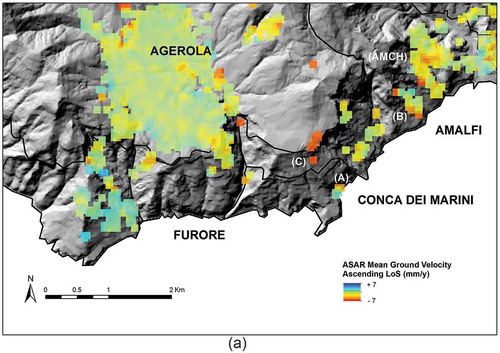
Figure 5. a) ASAR mean ground velocity map in Amalfi and Conca dei Marini; b) ASAR ground displacement time series for the selected sites (A, B, C and AMCH) obtained by meaning the adjacent pixels with ground velocity < –1 mm/y. c) 3D reconstruction of ASAR mean ground velocity in Conca dei Marini; d) 3D reconstruction of ASAR mean ground velocity of in Amalfi.

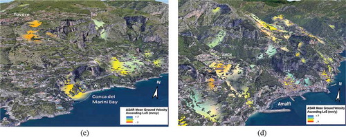
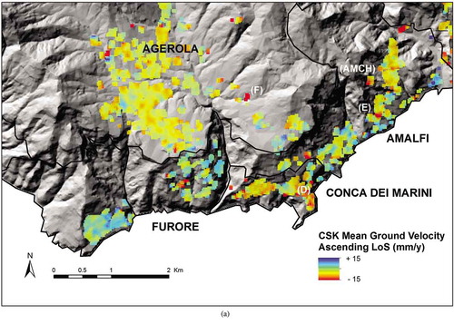
Figure 6. a) CSK mean ground velocity map in Amalfi and Conca dei Marini; b) CSK ground displacement time series for the selected sites (D, E, F and AMCH) obtained by meaning the adjacent pixels with ground velocity < −1 mm/y.

3. Airborne photo interpretation and fieldwork

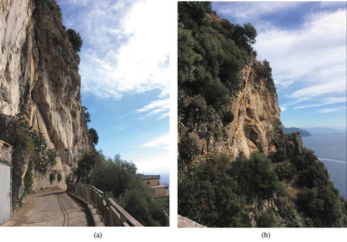
The deformation areas detected by the InSAR technique in Amalfi and Conca dei Marini municipalities have been investigated through airborne photo interpretation and subsequently through investigation in the field. The interpretation was based on aerial images acquired at the scale of 1:40,000 by BLOM CGR S.p.A (Compagnia Generale Riprese Aeree http://www.cgrspa.com/) during a 2006 flight. The analogic stereoscopy technique has been applied to 6 aerial images with spatial resolution of 1 m and covering an extent of 16 km². Thanks to the relief exaggeration technique (vertical amplification of 3x), the stereoscopic view allowed to distinguish geomorphological evidences related to slope instability phenomena outlined in Figure 7. Debris flows (in green) and debris avalanches (in orange) are identified in the upper sectors of the investigated area and in correspondence with the main joint-sets and tectonic features (i.e. faults and folds) on both sides of canyons located in the NW and SE sectors of the image. These two typologies of landslides could represent a particular evolving mechanism of massive rock-falls. The rock-fall accumulation zones (pink areas) are well identified on the coast and probably involve toppling phenomena occurred at different elevations in the back cliffs. Finally, the rock-fall calcareous scarps (in red) show linear trends parallel and perpendicular to the coastline and could be influenced by the low-stand of the sea controlled by some tectonic features (faults system) characterized by NW-SE and NE-SW trends as shown in Figure 1. After the photo-geological interpretation, these areas have been checked during a field survey carried out on September 28–29, 2015. In detail, 9 Ground Control Points (GCPs) were individuated and surveyed (Table 4 and Figure 8). The relative plano-altimetric coordinates have been retrieved with the GPS-RTK (Global Positioning System – Real Time Kinematics) technique based on the signals transmitted by satellite systems (GPS, GLONASS, Galileo) and on two signal receivers (mobile and reference stations) that acquire the GCPs coordinates with horizontal (x, y) and vertical (z) accuracy of 1 and 2 cm, respectively. In particular, the points recorded in Amalfi and Conca dei Marini municipalities have been corrected via GPRS/UMTS from the Fisciano CGPS reference station (RTCM-ID 35). The field survey reveals that the deformation areas detected by the InSAR processing (sites in Figures 5a and 6a) are characterized by morphological elements individuated also by photo-geological interpretation (Figure 7). In particular, the most relevant ground deformations are concentrated in the upper sector of Amalfi municipality (Site (B) in Figure 5a, Site (E) in Figure 6a, Site (1) in Figure 7 and picture in Figure 9a) and in the Conca dei Marini bay (Site (A) in Figure 5a, Site (D) in Figure 6a; Site (2) in Figure 7 and picture in Figure 9b). These areas show sub-vertical planes and isolated rock masses characterized by columnar and trapezoidal shapes linked to the joint-set system. These rock masses of huge dimensions can evolve into rock-falls and toppling phenomena causing disastrous consequences in the near inhabited zones. Areas potentially subjected to these phenomena are highlighted in Figure 5c where the (A) site is represented by the cliff above Conca dei Marini beach (Figure 9b) and in Figure 5d with the (B) site represented by the fractured rock block above the building area (Figure 9a).

Table 4. GPS reference stations and surveyed Ground Control Points (GCP) coded names and characteristics. Reference stations are equipped with Leica GRX1200+ receiver and LEIAT 504 antenna (choke ring). GCPs have been measured by Leica GX1230 receiver and LEIAX1202 antenna. The AMCH has been used as reference point in the GEP procedure during ASAR processing.

TYPE	CODE	Lat	Long	Ellipsoid Height (m)
Reference Station	FISC (Ref 0035)	40° 46ʹ 13.74380” N	14° 47ʹ 24.91181” E	309.97
Reference Station	SORR (Ref 0228)	40° 37ʹ 45.44149” N	14° 23ʹ 47.13702” E	131.74
GCP	CECI	40° 39ʹ 04.91717” N	14° 42ʹ 07.09366” E	220.62
GCP	CETA	40° 39ʹ 25.20402” N	14° 42ʹ 27.60510” E	173.67
GCP	CETB	40° 39ʹ 26.39523” N	14° 42ʹ 27.41213” E	173.08
GCP	CETC	40° 39ʹ 21.09330” N	14° 42ʹ 24.41803” E	172.89
GCP	AMCH	40° 38ʹ 14.14255” N	14° 35ʹ 34.79730” E	360.02
GCP	AUDI	40° 39ʹ 02.79838” N	14° 36ʹ 52.63663” E	373.87
GCP	CEBA2	40° 38ʹ 55.98605” N	14° 42ʹ 13.38502” E	84.33
GCP	RAVE	40° 39ʹ 01.24085” N	14° 36ʹ 58.60647” E	295.17
GCP	SCAL	40° 39ʹ 03.97808” N	14° 36ʹ 09.13341” E	561.55

Figure 7. Aerial image and interpretation of Amalfi and Conca dei Marini area. The numbers 1 and 2 indicate the position of the sites shown in Figures 9a and 9b, respectively. The inset shows the 6 aerial images coverage and their respective numbers.

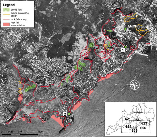
Figure 8. GPS surveyed points map.

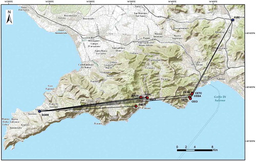
Figure 9. Fieldwork pictures; a) Amalfi upper sector above harbor site; b) Conca dei Marini bay site.

4. Landslide susceptibility index mapping

In order to extent the identification of the areas potentially subjected to slope instability in the entire territories of Amalfi and Conca dei Marini, the Landslide Susceptibility Index (LSI) is here developed. This index is based on the equation that combines the susceptibility parameters on a GIS platform (ESRI Environment, ArcGIS Deskstop 10.5). These parameters are stored in a geospatial matrix (ESRI GRID) having coherent spatial resolution with the LiDAR DEM (2 m cell size). The following equation is used to calculate the Index:

(1) $\mathrm{L}\mathrm{S}\mathrm{I}=\sum _{j=1}^m\sum _{i=1}^n\left(p_{\mathrm{i}}\ast w_{ij}\right)$(1)

where i represents the selected parameter and j is its class, Pi is the weight of the selected parameter (primary weight) and wij is the weight of each class j belonging to each parameter i (relative weight).

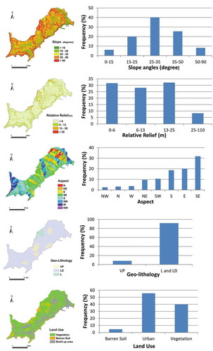
The susceptibility parameters were selected according to their capacity to be destabilizing factors (Montgomery and Dietrich 1994; Brenning 2008). They are: slope, relative relief, aspect, geo-lithology and land use. The Slope (SL), Relative Relief (RR) and Aspect (A) are morphometric parameters derived from high resolution (2 m) Digital Elevation Models (DEMs) obtained by Airborne Lidar data (Pizzimenti et al. 2016), whereas the Geo-Lithology (L) and the Land Use (LU) are derived from raster cartography and multispectral satellite data, respectively (Bisson et al. 2013a; Bisson, Spinetti, and Sulpizio 2014).

• The Slope parameter has been calculated applying formula of Burrough and Mc-Donell (1998) to the DEM. The Slope is the morphometric parameter that most influences the instability of the terrain since it controls directly the balance between resistant and gravitational forces causing any type of landslide (Mejià-Navarro et al. 1994; Bovis and Jakob 1999). In particular, the surface slope plays a key role as a predisposing factor for both rock fall and volcanoclastic debris flow triggering. In the case of rock fall, according to Dorren (2003), rock freefall occurs if the slope gradient exceeds 76°; for values around 70° the rock motion ranges from falling to bouncing and for values around 45° the rocks begin to roll. Anyway, literature data confirm that most of rock fall occur with slopes greater than 50° (Marquinez et al. 2003). In the case of volcanoclastic debris flows, the triggering slopes can range from 25° (minimum slope following the model of Takahashi 2000) to 45° (limit of internal slope angle of granular deposits). In particular, the events recorded on the Peninsula involve volcanic fall out deposits mantling the carbonatic bedrock with slopes generally between 25° and 35° (De Riso et al. 1999; Calcaterra et al. 1999, 2000; Pareschi et al. 2000; De Vita, Agrello, and Ambrosino 2006) even if recent studies (Bisson et al. 2013b) individuated lower triggering thresholds (< 25°).

• The Relative Relief is a parameter that quantifies the relief energy and strongly influences the potential triggering of the landslides since it is linked to the erosion activity (Vergari et al. 2011). The parameter is defined as the elevation range within a specific area and in this study, it has been calculated from the DEM by subtracting the minimum elevation matrix from the maximum elevation matrix and using a 3 × 3 window.

• The Aspect indicates the exposure of the face surface defined by the direction of slope maximum and has an indirect influence on slope instability. The zones exposed southward are affected by a greater thermal diurnal cycling due to the exposure to sun radiation that increases the slope face temperature. In the boreal hemisphere, the zones exposed northward are often shaded, while the ones exposed southward receive more solar radiation for a specific surface area. This may also influence the amount of humidity absorbed by the exposed face. Both thermal stress and humidity may favor erosion activity. Moreover, surfaces exposed to the South present lower vegetation density compared to surfaces exposed to the North (Bennie et al. 2006). The growth of vegetation roots helps to keep terrain material in place (De Baets et al. 2006). Due to the paucity of protective vegetation cover (Pimentel and Kounang 1998), south and southeastern exposed areas are subject to more erosion and therefore are potentially unstable.

• The Geo-Lithology parameter derives from the geological raster cartography at the scale 1:25,000 (Bisson et al. 2013a) covering the entire Sorrentina Peninsula. The digitized polygon features were grouped into 8 main typologies according to similar lithological characteristics: Cretaceous limestone series (L), Oligocene clay shale (OL2); Jurassic calcareous dolomitic series (LD), Quaternary pudding stones and breccia (Q), Recent alluvial deposits (A), Reworked volcanic products and slope debris (RVP), Triassic marly dolomitic calcareous series (MDL), Volcanic products (VP). Subsequently, the vector layer relative to Amalfi and Conca dei Marini was extrapolated and transformed into a georeferenced raster coherent with the spatial resolution and extent of the other parameters. The role of the geo-lithology parameter in landslide occurrence is evidenced by Apuzzo et al. (2013) and Budetta (2010). In detail, the rock falls recorded on the Peninsula affect the calcareous sequences (LD and L) often characterized by structural-slopes and fault-slopes. This suggests that high-energy calcareous slope and rock-mass fracturing can be considered rock fall predisposing factors, especially if combined with thermo-weathering, karst phenomena and marine erosion, phenomena that occur frequently on the Peninsula. Instead, the volcaniclastic debris flows are triggered on steep slopes of carbonate bedrock mantled by pyroclastic deposits, often reworked (VP and RVP) and with variable thickness (De Vita et., 2006; Del Soldato et al. 2018). During heavy or prolonged rainfall (e.g. Onorati, Braca, and Liritano 1999) these deposits become shallow landslides that rapidly move under the influence of gravity on the impermeable carbonate substratum transforming into volcanoclastic debris flows.

• The Land Use (LU) has been obtained by analyzing the NASA Landsat 5 scene acquired in 19–10-1997. The scene has been processed to obtain the 3 main classes of Land Cover: barren soil, vegetation and build-up areas. The vegetation and bare soil maps have been derived by applying the NDVI (Normalized Difference Vegetation Index, Crippen 1990) and NDBSI (Normalized Difference Soil Index, Baraldi et al. 2006). NDVI uses band 4 (b4) and band 3 (b3) and is calculated according to the following relation: ([b4 – b3]/[b4 + b3]), whereas the NDSI uses band 5 (b5) and band 3 (b3) and is calculated according to the following formula: ([b5-b3]/[b5 + b3]). The map of the build-up areas has been derived by subtracting the NDVI and NDSI maps from the initial image. In order to maintain spatial resolution coherent to the DEM resolution, the three maps have been resampled at 2 m and transformed into a vector polygon layer. Subsequently they were checked by using 1 m resolution airborne images acquired during 1997–1998 by the AIMA (State Agency for Interventions on the Agricultural Market) (Bisson, Spinetti, and Sulpizio 2014). Finally, the three vector layers have been merged to create the Land Use map.

4.1. Multivariate analysis

For each susceptibility parameter used in the LSI, a multivariate analysis was applied to individuate the classes and the respective weights (Figure 10). In detail, the values assumed by each parameter in the deformation areas characterized by mean ground velocities < -1 mm/y have been analyzed with frequency histograms to individuate significant thresholds and the relative classes. These classes have been compared and combined with the literature classes in order to assign the final weight to each class (Bisson, Spinetti, and Sulpizio 2014 and references therein). Table 5 reports for each susceptibility parameter (i) the weight (primary weight) and the classes (j) with the respective weights (relative weight). Since the Slope is recognized as the main predisposing factor to instability we have assigned the maximum weight of 10. For this parameter the statistical analysis has confirmed the 5 classes already individuated by previous studies (Bisson, Spinetti, and Sulpizio 2014). The second predisposing factor to instability is the Relative Relief directly connected to the slope. The weight of this factor depends on the dimensions of the calculation window that, in this study, covers an area of 6m x 6m. For this reason, we have assigned a primary weight comparable to the Slope weight, whereas the classes and the respective weights have been defined by analyzing the relative frequency histogram (Table 5). As a third parameter, we have selected Geo-Lithology. This parameter does not directly cause the triggering of the landslide, but influences the typology of landslides that can occur. In fact, a very cohesive and compact lithology is more prone to be fractured to generate rock falls, whereas incoherent and loose deposits favor sliding or flow phenomena. Regardless, in both lithology types, a triggering factor it is necessary as intense or prolonged rainfall, earthquakes, volcanic activity or multiple human actions. Taking into account these considerations, Table 5 reports the primary and relative weights of the Geo-Lithology. The last two susceptibility parameters are Land Use and Aspect. The weights and the respective classes assigned to the Land Use have been defined considering their major or minor influence on slope instability according to literature data (Reichenbach et al. 2014). Barren soil is the type of land cover more exposed to rain and wind, which are the two primary causes of surface erosion (Pimentel and Kounang 1998).Vegetation stabilizes loose deposits (Gyssels and Poesen 2003) whereas built-up areas interfere with the gravity equilibrium of loose deposits (Vrieling 2006). As a consequence, the highest weight of this parameter was assigned to barren soil, followed by vegetation and then built-up areas (Table 5). Finally, the weight assigned to Aspect is slightly higher than the Land Cover weight (Table 5). The influence of Aspect in landslide generation can change according to the Land Use present in the investigated area. Nonetheless, its influence is always strongly dependent on the slope. In this study, two classes of Aspect (Table 5) were defined considering exposure to sun radiation and according to considerations already discussed previously.

Table 5. LSI parameters. For each selected parameter the table reports the acronym the assigned weight (Pi), the classes (j) with the respective weights (Wij).

		Landslide
Parameters (i)	Acronym	Pi	j	Wij
			SL < 15°	1
			15°≤ SL < 25°	3
Slope	SL (degrees)	10	25°≤ SL < 35°	8
			35°≤ SL < 50°	9
			SL ≥ 50°	10
			RR < 6	5
			6 ≤ RR < 13	7
Relative Relief	RR (m)	9	13 ≤ RR < 25	9
			RR ≥ 25	10
			L	9
Geo-Lithology	L	8	LD	8
			VP	10
Aspect	A	6	S, SE, SW E,	8
			N, NE, NW, W	4
			Build up area	5
Land Use	LU	7	Vegetation	6
			Barren soil	8

Figure 10. Susceptibility parameters statistical histograms in the deformation areas of Amalfi and Conca dei Marini.

5. Results and discussion

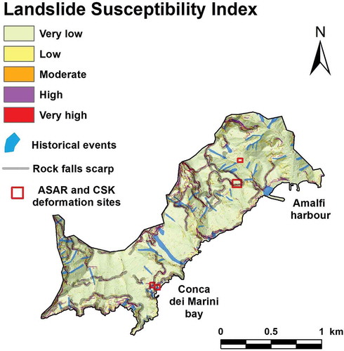
The resulting 2 m high resolution LSI map classifies thoroughly Conca dei Marini municipality and almost the entire territory of Amalfi into 5 classes of susceptibility (Figure 11). The 5 classes were defined by the Jenk’s method applied to the entire range of LSI values (from 69 to 291) derived from equation (1). The very low instability class covers almost 80% of all the investigated area, whereas the others four classes cover the 20%. In detail, the high and very high LSI areas affect 6% of the investigated territory (red and purple areas in Figure 11).

In order to achieve the quality of landslide susceptibility map, as suggested by Guzzetti et al. (2006), independent landslide data were introduced. A spatial analysis was conducted in the GIS environment by overlapping the vector map of the 2011 historical landslides with the LSI map. The areas classified at high/very high LSI indicate the potentially more exposed zones for triggering landslides. In fact, they correspond mostly to steep zones (slope angles between 25° and 70°) that fall inside or very close to the historical landslide upper boundary recognized as the landslide source zone. In order to test the reliability of the LSI map, its accuracy was calculated by analyzing the distances between the upper boundaries of historical landslides and the respective high/very high LSI zones. The planimetric error of the historical landslides map, as derived from a cartography at a scale of 1:5000, is ± 2 m, which is the same as the LSI map calculated by considering the propagation of planimetric errors of each susceptibility parameter. In detail, the planimetric error of morphometric parameters is ± 20 cm as derived from the accuracy of the LiDAR DEM data (Pizzimenti et al. 2016). The Land Use parameter assumes the same planimetric error for the high-resolution airborne AIMA images (± 2 m). With regards to Geo-Lithology, the planimetric error is 10 m as derived from the geological map at a scale of 1:25,000. This error can be considered negligible as more than 90% of the territory is characterized by the same type of lithological cover. Analyzing the distances between the 40 historical landslides and the areas at high and very high susceptibility, the LSI map prediction accuracy results equal to 85%.

In order to better constrain the potential source areas individuated by the LSI map, the slope instability peculiarities (e.g. scarps, very steep surfaces characterized by joints system, fractures) individuated by the photo-geological interpretation (Figure 7) and then checked in the field (Figure 9) were overlain on the LSI map (Figure 11). This spatial analysis provides evidence that all the instability elements fall in the high and very high LSI zones, confirming that those areas are most predisposed to landslide triggering.

To provide a quantitative analysis of the susceptibility areas, the deformation sites detected by ASAR and CSK data processing (Figures 5a and 6a) were superimposed on the LSI map (Figure 11). Those deformation sites fall in the high and very high susceptibility zones. In detail, the time series of the four sites (Figures 5b and 6b) individuated in Conca dei Marini bay and in the sector above the Amalfi harbor show similar values in the AMCH survey point and a general decreasing trend interrupted by not linear features. This trend indicates slow ground deformation, whereas the not linear features could be associated with weathering crust phenomena and seasonal effects that are particularly evident in the Tovere site (point C in Figure 5b). This slow deformation is also supported by low mean ground velocities between −6 mm/y and −4 mm/y for the ASAR dataset and between −15 mm/y and −9 mm/y for the CSK dataset. These elements indicate slow deformation constant in time, probably due to the well-known geo-structural context affecting the entire Peninsula (Apuzzo et al. 2013). Nevertheless, the areas characterized by the highest values of displacement, −58 mm in Conca dei Marini bay (point A Figure 5b) and −40 mm in the upper sector of Amalfi harbor (point E Figure 6b), result classified with high/very high LSI. This could suggest potential slope instability phenomena such as slipping along the terrain slope, landslides, or subsidence phenomena.

Figure 11. Amalfi and Conca dei Marini LSI resulting Map.

6. Conclusions

A GIS-based interdisciplinary approach involving Remote Sensing investigations, Geo-Lithological elements and Morphometric analyses, was applied to identify the areas in the Sorrentina Peninsula potentially more prone to trigger landslides. The Peninsula is a densely populated and touristic area that is frequently affected by such natural disasters. Multi-temporal InSAR analyses applied to the Envisat-ASAR (2003–2010) and COSMO-SkyMed (2013–2015) datasets identified Amalfi and Conca dei Marini as the municipalities most affected by ground deformation in the time window covered by the two datasets. In particular, four sites were detected in areas close to Amalfi and Conca dei Marini coast. These sites show deformations with the mean ground velocity values between −6 ± 1 mm/y and −4 ± 1 mm/y (ASAR) and between −15 ± 1 mm/y and −9 ± 1 mm/y (CSK). These velocities were derived from the respective time series that reveal maximum ground displacement values ranging from −55 ± 5 mm (ASAR case) to −40 ± 3 mm (CSK case). The identified sites, investigated by a photo-geological analysis combined with checks in the field, provide evidence of unstable geo-morphological elements such as rock-fall escarpments, detachment zones, steep surfaces with several multiple fractures, and rock masses with columnar and trapezoidal shapes generated by dense joint-set systems. All these elements, if subject to intensive rainfall or seismic events, could evolve into landslide phenomena.

The LSI Index developed here classifies the entire territory of Amalfi and Conca dei Marini municipalities into 5 different degrees of susceptibility with a prediction accuracy of 85%. The resulting LSI map shows that the high/very high LSI zones fall in the source areas of all historical landslides and are characterized by 25°-70° slope angles corresponding to steep zones with unstable geo-morphological elements such as the rock fall scarps identified by the photo-geological analysis. Finally, the ASAR and CSK deformation sites detected in Amalfi and Conca dei Marini are classified at high/very high susceptibility. These results demonstrate the high reliability of the LSI that, as shown here, may represent a useful tool for the prevention and mitigation of landslide hazards on Sorrentina Peninsula or in territories with geo-morphological characteristics similar to the areas investigated in this work.

Acknowledgements

This study was supported by the LCC project of INGV ‘Struttura Ambiente’ supervised by Dr. F. Florindo. The ground elevation data were kindly provided by ‘Provincia di Napoli’ and by ‘Ministero dell’Ambiente e della Tutela del Territorio e del Mare’. We are very grateful to Eng. G. D’Onofrio (Autorità di Bacino Regionale di Campania Sud), Dr. C.A. Brunori, Dr. L. Pizzimenti, Dr. A. Tadini and Dr. R. Gianardi for DEMs. We also thank Dr. S. Monna and Dr. A. Clarke for their useful review and the five anonymous reviewers that contributed to the clarity of the exposed work.

Disclosure statement

No potential conflict of interest was reported by the authors.

References

- Apuzzo, D., P. De Vita, B. Palma, and D. Calcaterra. 2013. “Approaches for Mapping Susceptibility to Rockfalls Initiation in Carbonate Rock-Masses: A Case Study from the Sorrento Coast (Southern Italy).” Italian Journal of Geosciences 132: 380–393. doi:10.3301/IJG.2013.12.
- Baraldi, A., V. Puzzolo, P. Blonda, L. Bruzzone, and C. Tarantino. 2006. “Automatic Spectral Rule-Based Preliminary Mapping of Calibrated Landsat TM and ETM+ Images.” IEEE Transactions on Geoscience and Remote Sensing 44 (9): 2563–2586. doi:10.1109/TGRS.2006.874140.
- Bennie, J. O., M. Hill, R. Baxter, and B. Huntley. 2006. “Influence of Slope and Aspect on Long-Term Vegetation Change in British Chalk Grasslands.” Journal of Ecology 94 (2): 355–368. doi:10.1111/jec.2006.94.issue-2.
- Berardino, P., G. Fornaro, R. Lanari, and E. Sansosti. 2002. “A New Algorithm for Surface Deformation Monitoring Based on Small Baseline Differential SAR Interferograms.” IEEE Transactions on Geoscience and Remote Sensing 40: 2375–2383. doi:10.1109/TGRS.2002.803792.
- Bisson, M., C. Spinetti, and R. Sulpizio. 2014. “Volcaniclastic Flow Hazard Zonation in the Sub-Apennine Vesuvian Area by Using GIS and Remote Sensing.” Geosphere 10 (6): 1419–1431. doi:10.1130/GES01041.1.
- Bisson, M., G. Fubelli, R. Sulpizio, and G. Zanchetta. 2013a. “A GIS-based Approach for Estimating Volcaniclastic Flow Susceptibility: A Case Study from Sorrentina Peninsula (Campania Region).” Italian Journal of Geosciences 132 (3): 394–404. doi:10.3301/IJG.2012.37.
- Bisson, M., G. Zanchetta, R. Sulpizio, and F. Demi. 2013b. “A Map for Volcaniclastic Debris Flow Hazards in Apennine Areas Surrounding the Vesuvius Volcano (Italy).” Journal of Maps 9 (2): 230–238. doi:10.1080/17445647.2013.768948.
- Bovenga, F., D. O. Nitti, G. Fornaro, F. Radicioni, A. Stoppini, and R. Brigante. 2013. “Using C/X-band SAR Interferometry and GNSS measurements for the Assisi Landslide Analysis.” International Journal of Remote Sensing 34 (11): 4083–4104.
- Bovenga, F., J. Wasowski, D. O. Nitti, R. Nutricato, and M. T. Chiaradia. 2012. “Using COSMO/SkyMed X-Band and ENVISAT C-Band SAR Interferometry for Landslides Analysis.” Remote Sensing of Environment 119: 272–285. doi:10.1016/j.rse.2011.12.013.
- Bovis, M. J., and M. Jakob. 1999. “The Role of Debris Supply Conditions in Predicting Debris-Flow Activity.” Earth Surface Processes and Landforms 24: 1039–1054. doi:10.1002/(ISSN)1096-9837.
- Brenning, A. 2008. “Statistical Geocomputing Combining R and SAGA: The Example of Landslide Susceptibility Analysis with Generalized Additive Models.” Hamburger Beiträge zur Physischen Geographie und Landschaftsökologie 19 (23–32): 410.
- Budetta, P. 2010. “Rockfall-Induced Impact Force Causing A Debris Flow on A Volcanoclastic Soil Slope: A Case Study in Southern Italy.” Natural Hazards and Earth System Sciences 10: 1995–2006. doi:10.5194/nhess-10-1995-2010.
- Budetta, P., R. De Riso, and A. Santo. 2005. “Landslide Hazard and Risk along the Campanian Roads (Italy).” Proceedings of Inten. Conf.“Géoline 2005”, 23–25 May, Lione, France, 1–13.
- Burrough, P. A., and R. A. McDonell. 1998. Principles of Geographical Information Systems, 190. New York: Oxford University Press.
- Bϋrgmann, R., P. A. Rosen, and E. J. Fielding. 2000. “Synthetic Aperture Radar Interferometry to Measure Earth’s Surface Topography and Its Deformation.” Annual Review of Earth and Planetary Sciences 28: 169–209. doi:10.1146/annurev.earth.28.1.169.
- Calò, F., F. Ardizzone, R. Castaldo, P. Lollino, P. Tizzani, F. Guzzetti, … M. Manunta. 2014. “Enhanced Landslide Investigations through Advanced DInSAR Techniques: The Ivancich Case Study, Assisi, Italy.” Remote Sensing of Environment 142: 69–82. doi:10.1016/j.rse.2013.11.003.
- Calcaterra, D., M. Parise, B. Palma, and L. Pelella. 1999. “The May 5th 1998, Landsliding Event in Campania (Southern Italy): Inventory of Slope Movements in the Quindici Area.” In Proceedings of International Symposium on Slope Stability Engineering, IS, Shikoku ’99, Matsuyama, Shikoku, Japan, November 8–11, 1999, edited by N. Yagi, T. Yamagami, and J. Jiang, 1361–1366. Rotterdam: Balkema.
- Calcaterra, D., M. Parise, B. Palma, and L. Pelella. 2000. “Multiple Debrisflows in Volcaniclastic Materials Mantling Carbonate Slopes.” In Debris-Flow Hazards Mitigation: Mechanics, Prediction, and Assessment, edited by G. F. Wieczorek and N. D. Naeser, 99–107. Rotterdam: Balkema.
- Calcaterra, D., and A. Santo. 2004. “The January 10, 1997 Pozzano Landslide, Sorrento Peninsula, Italy.” Engineering Geology 75: 181–200. doi:10.1016/j.enggeo.2004.05.009.
- Calcaterra, D., M. Parise, and B. Palma. 2003. “Combining Geological and Historical Data for the Assessment of the Landslide Hazard: A Case Study from Campania (Italy).” Natural Hazards and Earth System Sciences 3: 3–16. doi:10.5194/nhess-3-3-2003.
- Cascini, L., G. Fornaro, and D. Peduto. 2009. “Analysis at Medium Scale of Low-Resolution DInSAR Data in Slow-Moving Landslide-Affected Areas.” ISPRS Journal of Photogrammetry and Remote Sensing 64 (6): 598–611. doi:10.1016/j.isprsjprs.2009.05.003.
- Cascini, L., G. Fornaro, and D. Peduto. 2010. “Advanced Low- and Full-Resolution DInSAR Map Generation for Slow-Moving Landslide Analysis at Different Scales.” Engineering Geology 112 (1–4): 29–42. doi:10.1016/j.enggeo.2010.01.003.
- Casu, F., M. Manzo, and R. Lanari. 2006. “A Quantitative Assessment of the SBAS Algorithm Performance for Surface Deformation Retrieval from DInSAR Data.” Remote Sensing of Environment 102: 195–210. doi:10.1016/j.rse.2006.01.023.
- Cioni, R., A. Longo, G. Macedonio, R. Santacroce, A. Sbrana, R. Sulpizio, and D. Andronico. 2003. “Assessing Pyroclastic Hazard through Field Data and Numerical Simulations: Example from Vesuvius.” Journal of Geophysical Research 108: 2063. doi:10.1029/2001JB000642.
- Colesanti, C., A. Ferretti, C. Prati, and F. Rocca. 2003. “Monitoring Landslides and Tectonic Motions with the Permanent Scatterers Technique.” Engineering Geology 68: 3–14. doi:10.1016/S0013-7952(02)00195-3.
- Colesanti, C., and J. Wasowski. 2006. “Investigating Landslides with Space-Borne Synthetic Aperture Radar (SAR) Interferometry.” Engineering Geology 88 (3–4): 173–199. doi:10.1016/j.enggeo.2006.09.013.
- Corsini, A., P. Farina, G. Antonello, M. Barbieri, N. Casagli, F. Coren, and D. Tarchi. 2006. “Space‐Borne and Ground‐Based SAR Interferometry as Tools for Landslide Hazard Management in Civil Protection.” International Journal of Remote Sensing 27 (12): 2351–2369. doi:10.1080/01431160600554405.
- Crippen, R. E. 1990. “Calculating the Vegetation Index Faster.” Remote Sensing of Environment 34 (1): 71–73. doi:10.1016/0034-4257(90)90085-Z.
- De Baets, S., J. Poesen, G. Gyssels, and A. Knapen. 2006. “Effects of Grass Roots on the Erodibility of Topsoils during Concentrated Flow.” Geomorphology 76: 54–67. doi:10.1016/j.geomorph.2005.10.002.
- De Riso, R., P. Buretta, D. Calcaterra, and A. Santo. 1999. “Le colate rapide in terreni piroclastici del territorio campano.” In Atti Convegno Previsione e prevenzione di movimenti franosi rapidi, 133–150. Trento, 17–19 giugno 1999.
- De Vita, P., D. Agrello, and F. Ambrosino. 2006. “Landslide Susceptibility Assessment in Ash-Fall Pyroclastic Deposits Surrounding Mount Somma-Vesuvius: Application of Geophysical Surveys for Soil Thickness Mapping.” Journal of Applied Geophysics 59 (2): 126–139. doi:10.1016/j.jappgeo.2005.09.001.
- Del Soldato, M., V. Pazzi, S. Segoni, P. De Vita, V. Tofani, and S. Moretti. 2018. “Spatial Modeling of Pyroclastic Cover Deposit Thickness (Depth to Bedrock) in Peri‐Volcanic Areas of Campania (Southern Italy).” Earth Surface Processes and Landforms 43 (9): 1757–1767. doi:10.1002/esp.v43.9.
- Dorren, L. K. A. 2003. “A Review of Rockfall Mechanics and Modelling Approaches.” Progress in Physical Geography 27 (1): 69–87. doi:10.1191/0309133303pp359ra.
- Esposito, E., S. Porfido, and C. Violante. 2004. “Il nubifragio dell’ottobre 1954 a Vietri sul Mare-Costa di Amalfi, Salerno.” Scenario ed effetti di una piena fluviale catastrofica in un’area di costa rocciosa. Pubbl. GNDCI n. 2870, ISBN 88-88885-03-X.
- García-Davalillo, J. C., G. Herrera, D. Notti, T. Strozzi, and I. Álvarez-Fernández. 2014. “DInSAR Analysis of ALOS PALSAR Images for the Assessment of Very Slow Landslides: The Tena Valley Case Study.” Landslides 11 (2): 225–246. doi:10.1007/s10346-012-0379-8.
- Guzzetti, F., A. C. Mondini, M. Cardinali, F. Fiorucci, M. Santangelo, and K. T Chang. 2012. “Landslide Inventory Maps: New Tools for an Old Problem.” Earth-Science Reviews 112 (1–2): 42–66. doi:10.1016/j.earscirev.2012.02.001.
- Guzzetti, F., P. Reichenbach, F. Ardizzone, M. Cardinali, and M. Galli. 2006. “Estimating the Quality of Landslide Susceptibility Models.” Geomorphology 81 (1–2): 166–184. doi:10.1016/j.geomorph.2006.04.007.
- Gyssels, G., and J. Poesen. 2003. “The Importance of Plant Root Characteristics in Controlling Concentrated Flow Erosion Rates.” Earth Surface Processes and Landforms 28: 371–384. doi:10.1002/(ISSN)1096-9837.
- Herrera, G., F. Gutiérrez, J. C. García-Davalillo, J. Guerrero, D. Notti, J. P. Galve, ... and G. Cooksley. 2013. “Multi-sensor Advanced DInSAR monitoring of very slow landslides: The Tena Valley case Study (Central Spanish Pyrenees).” Remote Sensing of Environment 128: 31–43.
- Hooper, A. 2008. “A Multi‐Temporal InSAR Method Incorporating Both Persistent Scatterer and Small Baseline Approaches.” Geophysical Research Letters 35 (16). doi:10.1029/2008GL034654.
- Jaboyedoff, M., T. Oppikofer, A. Abellán, M. H. Derron, A. Loye, R. Metzger, and A. Pedrazzini. 2012. “Use of LIDAR in Landslide Investigations: A Review.” Natural Hazards 61 (1): 5–28. doi:10.1007/s11069-010-9634-2.
- Lucà, F., D. D’Ambrosio, G. Robustelli, R. Rongo, and W. Spataro. 2014. “Integrating Geomorphology, Statistic and Numerical Simulations for Landslide Invasion Hazard Scenarios Mapping: An Example in the Sorrento Peninsula (Italy).” Computers & Geosciences 67: 163–172. doi:10.1016/j.cageo.2014.01.006.
- Marquinez, J., R. M. Duarte, P. Farias, and M. J. Sanchez. 2003. “Predictive GIS-based Model of Rockfall Activity in Mountain Cliffs.” Natural Hazards 30 (3): 341–360. doi:10.1023/B:NHAZ.0000007170.21649.e1.
- Massonnet, D., K. Feigl, M. Rossi, and F. Adragna. 1994. “Radar Interferometric Mapping of Deformation in the Year after the Landers Earthquake.” Nature 369: 227–230. doi:10.1038/369227a0.
- Mejìa-Navarro, M., E. W. Wohl, and S. D. Oaks. 1994. “Geological Hazards, Vulnerability and Risk Assessment Using GIS: Model for Glenwood Spring, Colorado.” Geomorphology 10: 331–354. doi:10.1016/0169-555X(94)90024-8.
- Metternicht, G., L. Hurni, and R. Gogu. 2005. “Remote Sensing of Landslides: An Analysis of the Potential Contribution to Geo-Spatial Systems for Hazard Assessment in Mountainous Environments.” Remote Sensing of Environment 98 (2–3): 284–303. doi:10.1016/j.rse.2005.08.004.
- Montgomery, D. R., and W. E. Dietrich. 1994. “A Physically Based Model for the Topographic Control on Shallow Landsliding.” Water Resources Research 30 (4): 1153–1171. doi:10.1029/93WR02979.
- Onorati, G., G. Braca, and G. Liritano. 1999. “Evento idrogeologico del 4, 5 e 6 maggio 1998 in Campania. Monitoraggio ed analisi idrologica.” Atti dei Convegni Lincei – Accademia Nazionale dei Lincei 154: 103–108.
- Pareschi, M. T., M. Favalli, F. Giannini, R. Sulpizio, G. Zanchetta, and R. Santacroce. 2000. “May 5, 1998, Debris Flows in Circumvesuvian Areas (Southern Italy): Insights for Hazard Assessment.” Geology 28: 639–642. doi:10.1130/0091-7613(2000)28<639:MDFICA>2.0.CO;2.
- Pimentel, D., and N. Kounang. 1998. “Ecology of Soil Erosion in Ecosystems.” Ecosystem 1 (5): 416–426. doi:10.1007/s100219900035.
- Pizzimenti, L., A. Tadini, R. Gianardi, C. Spinetti, M. Bisson, and C. A. Brunori. 2016. “Digital Elevation Models Derived by ALS Data: Sorrentina Peninsula Test Areas.” Rapporti Tecnici 361, ISSN 2039–7941, 1–28.
- Porfido, S., E. Esposito, F. Alaia, F. Molisso, and M. Sacchi. 2009. “The Use of Documentary Sources for Reconstructing Flood Chronologies on the Amalfi Rocky Coast (Southern Italy).” Geological Society, London, Special Publications 322 (1): 173–187. doi:10.1144/SP322.8.
- Raspini, F., S. Bianchini, A. Ciampalini, M. Del Soldato, L. Solari, F. Novali, S. Del Conte, A. Rucci, A. Ferretti, and N. Casagli. 2018. “Continuous, Semi-Automatic Monitoring of Ground Deformation Using Sentinel-1 Satellites.” Scientific Reports 8: 7253. doi:10.1038/s41598-018-25369-w.
- Reichenbach, P., C. Busca, A. C. Mondini, and M. Rossi. 2014. “The Influence of Land Use Change on Landslide Susceptibility Zonation: The Briga Catchment Test Site (Messina, Italy).” Environmental Management 54 (6): 1372–1384. doi:10.1007/s00267-014-0357-0.
- Singhroy, V., and K. Molch. 2004. “Characterizing and Monitoring Rockslides from SAR Techniques.” Advances in Space Research 33 (3): 290–295. doi:10.1016/S0273-1177(03)00470-8.
- Slob, S., and R. Hack. 2004. “3-D Terrestrial Laser Scanning as a New Field Measurement and Monitoring Technique. In: Engineering Geology for Infrastructure Planning in Europe: A European Perspective.” edited by: Hack, R., R. Azzam, and R. Charlier, Lectures Notes in Earth Sciences, 179–189. Vol. 104. Berlin/Heidelberg: Springer.
- Takahashi, T. 2000. “Initiation and Flow of Various Types of Debris Flow.” In Proceedings Second International Conference on Debris Flow Hazards Mitigation: Mechanics Prediction and Assessment, edited by G. F. Wieczoreck, 15–25. Taipei.
- Trigilia, A., and C. Iadanza. 2007. IFFI. http://www.isprambiente.gov.it/files/progetti/Trigila_APAT.pdf
- Vergari, F., M. Della Seta, M. Del Monte, P. Fredi, and E. Lucia Palmieri. 2011. “Landslide Susceptibility Assessment in the Upper Orcia Valley (Southern Tuscany, Italy) through Conditional Analysis: A Contribution to the Unbiased Selection of Causal Factors.” Natural Hazards Earth System Science 11: 1475–1497. doi:10.5194/nhess-11-1475-2011.
- Vrieling, A. 2006. “Satellite Remote Sensing for Water Erosion Assessment: A Review.” Catena 65: 2–18. doi:10.1016/j.catena.2005.10.005.