A probabilistic fusion of a support vector machine and a joint sparsity model for hyperspectral imagery classification

Abstract

Hyperspectral imagery (HSI) is now in use for a wide range of applications such as land cover classification, climate change studies and environmental monitoring; however, the acquisition of HSI is still costly, and the curse of dimensionality i.e. the phenomenon that the amount of required training samples increases exponentially as the dimensionality increases linearly, makes it difficult to exploit the full potential of machine learning in HSI classification. To resolve the problem, we propose a novel framework for spatial-spectral HSI classification in this article. A soft support vector machine (SVM) and a probabilistic joint sparsity model (JSM) are proposed to compute a posteriori probabilities of the test pixels, respectively; and the probability scores are then fused by a linear opinion pool. Furthermore, a Markov random field (MRF) model is used as a maximum a posteriori (MAP) segmentation method for further regularization of the neighbor information to derive the labels for pixels. Extensive experiments conducted on three commonly-used benchmarking data sets show that the proposed probabilistic fusion method outperforms a number of well-known spatial-spectral HSI classification techniques.

Keywords:

• Hyperspectral imagery (HSI)
• classification
• support vector machine (SVM)
• joint sparsity model (JSM)
• Markov random field (MRF)
• decision fusion

1. Introduction

Hyperspectral imagery (HSI) has been known as a useful source for understanding the scene of remotely sensed data. Many methods have been introduced to perform HSI classification using the rich spectral information available in the images. For example, random forest (RF) (Ham et al. 2005), support vector machines (SVMs) (Mountrakis, Im, and Ogole 2011; Melgani and Bruzzone 2004) and neural network (NN) (Ratle, Camps-Valls, and Weston 2010) have achieved some competitive results. However, the insufficient training samples in contrast to the high dimensionality are the main obstacles to achieving high-accuracy HSI classification (Plaza et al. 2009). The higher dimensionality of HSI leads to the curse of dimensionality which is also known as Hughes phenomenon that the amount of required training samples increases exponentially as the dimensionality increases linearly (Landgrebe 2005).

Figure 4. Classification maps obtained by different classifiers for Data II with 9 classes: (a) SVM-EMAP; (b) SVM-MRF; (C) SR-MRF; (d) JSM; (e) JSM-MRF; (f) Proposed.

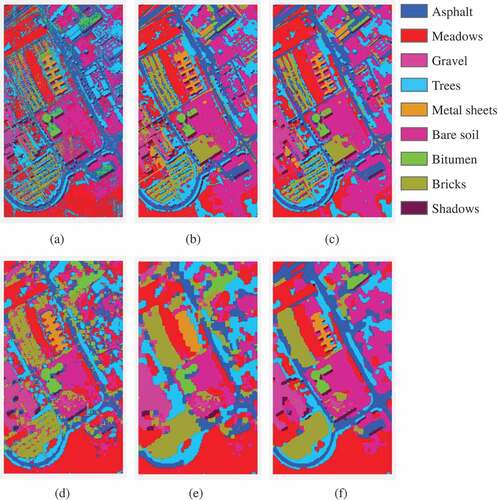
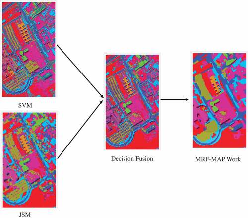
Figure 7. Classification maps of Data II after SVM, JSM and fusion.

On the other hand, SVMs with kernel functions can be applied to overcome the dimensionality problem by projecting the pixels into a high dimensional feature space and the decision boundary can be finally expressed as a function of a subset of training samples (Gualtieri and Cromp 1999; Huang, Davis, and Townshend 2002; Gao et al. 2015). In fact, SVMs have been widely used in HSI applications in this context. For example, (Xun and Wang 2015) adopted an object-based SVM method that incorporates an optimal segmentation scale estimation strategy for mapping salt cedar with QuickBird imagery. (Lin and Yan 2016) combined a polynomial kernel function and a radial basis kernel function to form a new kernel function-based SVM model for HSI classification. (Chu et al. 2016; Zhang, Smith, and Fang 2018) utilized SVMs to classify the fused images of lidar and HSI for tea classification and urban land-cover mapping, respectively. (Tesfamichael et al. 2018) used SVM to identify plant invasions by classifying raw hyperspectral and simulated multispectral images. Moreover, due to the presence of mixed pixels in the data, probabilistic SVMs have been used for the estimation of class-wise probability for each pixel in HSI classification (Villa et al. 2011; Jia et al. 2010). This kind of classification is also known as soft classification. The results from a soft classification method can induce the probability of the presence of each class in the pixel, and the results can be further processed by other probabilistic methods.

As can be seen in (Srinivas et al. 2013; Chen, Nasrabadi, and Tran 2013; Fu et al. 2017), another category of strategies to deal with the high dimensionality of HSI has been exploited by using sparse representation (SR). SR assumes that HSI pixels that belong to the same class lie in a same subspace formed from the training samples. In SR, a so-called “dictionary” is constructed by the training samples, and the labeling of test pixels can be determined by recovering the coefficients corresponding to the weight values of the selected elements from the dictionary. In order to better explore the merits of SR in HSI classification, a joint sparsity model (JSM) (Chen, Nasrabadi, and Tran 2011) was proposed to process the spatial contextual information of HSI. JSMs assume that a test pixel has the similar properties with its neighboring pixels. Based on the SR theory, the neighboring pixels can be simultaneously expressed by a few elements selected from the defined dictionary. The spatial information is utilized in this way by involving the neighboring pixels. JSMs have achieved very competitive results for HSI classification (Chen, Nasrabadi, and Tran 2011; Fang et al. 2014) in recent years. In the report of (Gao, Lim, and Jia 2018a), a JSM was adopted as a probabilistic classifier, and then a probabilistic relaxation method was successfully applied to improve the results for HSI classification. Some variations such as (Tu et al. 2018b, 2018a) have also been successfully applied for this classification topic.

It is well known that Markov random fields (MRFs) can help smooth over the hyperspectral data and reduce the noise. After a soft classification, an MRF is usually applied to explore the continuity of labels of neighboring pixels. The involvement of spatial contextual information is realized by assigning an appropriate weight to the spatial contribution of neighboring pixels around the central pixel in the minimization of an energy function. It is important to choose an appropriate MRF representation for the labeling process, and the maximum a posteriori (MAP) strategy has been widely used to represent the MRF energy function (Cao et al. 2017; Li, Bioucas-Dias, and Plaza 2012). In (Tarabalka et al. 2010; Moser and Serpico 2013), the results obtained by a pixel-wise probabilistic SVM was refined by some variations of MRFs. In the work of (Cao et al. 2017), a MRF was used to model the local spatial correlation of neighboring pixels and refine the probabilistic results based on the 3-dimensional discrete wavelet transform features that were obtained by a soft SVM. In (Zhang et al. 2018), semantic representation-based multiple features were extracted by a probabilistic SVM and an extended MRF was proposed to process the information in a semantic space. Probabilistic SR has also been integrated with an MRF (Xu and Li 2014) recently for high-accuracy HSI classification. More information about recent advances of this technique can be found in (Ghamisi et al. 2018).

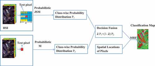
SVMs and JSMs are both successful machine learning techniques for HSI classification. However, SVMs in HSI classification are prone to errors since classes are likely to lie in a lower space than the original data dimension where SVMs cannot have sufficient training samples. Moreover, the constructed dictionary for a JSM may not be complete, which can lead to a compromised classification accuracy, and the over-smoothing effect limits the performance of JSMs in non-homogenous areas. To alleviate the negative impact of these problems, and to keep a balance between the high dimensionality and the limited training samples in HSI classification, we propose a novel framework that integrates both JSM and SVM methods in a probabilistic way. Specifically, an SVM is applied to process the spectral information and obtain a global probability distribution for all test pixels. Then, a JSM is introduced to integrate the spatial information and obtain a probability distribution for test pixels with local information involved. That is, we use the SVM and JSM methods to obtain a posteriori probabilities and fuse them with a linear opinion pool. Finally, an MRF as a maximum a posteriori (MAP) segmentation method is applied to regularize the final probabilities and model the spatial contextual information. The probability distribution obtained by the proposed SVM is based on the global spectral information, and the proposed JSM integrates the spatial information in a local neighborhood for the test pixels. The spatial contextual information characterized by an MRF-MAP can further help reduce the negative effect of insufficient training samples. Therefore the main contributions of this work are twofold: 1) taking the probabilistic information at spectral and spatial levels into account, and 2) the fusion strategy along with the characterization of spatial information that can maximize the classification accuracy.

The rest of this paper is composed of three sections: Section 2 describes the proposed framework, Section 3 shows the experimental results as well as discussion of some relevant parameters, and Section 4 draws the conclusion.

2. Fusion of support vector machine and joint sparsity model

The workflow of the proposed framework is shown in Figure 1 in detail. It comprises four steps: 1) generation of a probabilistic distribution of the test pixels via a probabilistic SVM; 2) generation of a posteriori probability distribution of the test pixels via a probabilistic JSM; 3) fusion of the probabilistic distributions obtained in the previous steps; 4) regularization via an MRF-MAP. The details for each step are presented in the following subsections.

Figure 1. The illustration of the proposed fusion algorithm that integrates JSM and SVM in a probabilistic sense for HSI classification.

2.1. Probabilistic joint sparsity model

According to the principle that HSI pixels tend to have a common sparsity pattern with their neighbors, the spatial correlation among pixels can be exploited by a JSM (Chen, Nasrabadi, and Tran 2011).

Let $I$ be a HSI cube, and $x_i\in {\mathbb{R}}^{L\times 1}$ be a pixel in the image cube with $L$ representing the spectral dimensionality. Based on SR, $x_i$ can be expressed as:

(1) $x_i=D{r}_i$(1)

where $D=[D_1,...,D_c,...,D_C]\in {\mathbb{R}}^{L\times N}$ is the structural dictionary constructed from the training samples, $D_c\in {\mathbb{R}}^{L\times N_c}$ is the c-th sub-dictionary, and $c=1,...,C$ denotes the predefined class labels. $N=\sum _{c=1}^C{N}_c$ denotes the total number of elements in the whole dictionary, $N_c$ corresponds to the number of elements in the c-th sub-dictionary, and $r_i\in {\mathbb{R}}^{N\times 1}$ denotes the sparse coefficient vector for the pixel $x_i$.

The sparse coefficient vector $r_i$ can be computed as:

(2) ${\hat{r}}_i=\underset{r_i}{argmin}{∥x-D{r}_i∥}_2\mathrm{s}\mathrm{u}\mathrm{b}\mathrm{j}\mathrm{e}\mathrm{c}\mathrm{t}\mathrm{t}\mathrm{o}{∥r_i∥}_0\le K$(2)

where $K$ and ${∥r_i∥}_0$ are the upper bound and the total number of nonzero rows in $r_i$, respectively.

A JSM (Chen, Nasrabadi, and Tran 2011) that extends Equation (1) to a neighborhood region was proposed on the assumption that the pixel$x_i$ shares a common sparsity pattern with its neighboring pixels. Let $X=\{x_i\},i=1,2,...,W\times W$ be the pixels within a predefined neighborhood region with a center at $x_i$, and $W\times W$ is the predefined neighborhood region size. Equation (1) can be re-defined as:

(3) $\begin{array}{c}X=[D{r}_1,D{r}_2,...,D{r}_{W\times W}]\\ =DR\end{array}$(3)

where $R\in {\mathbb{R}}^{N\times W^2}$ denotes the sparse coefficient matrix, and it is recovered in this paper as:

(4) $\hat{R}=\underset{R}{argmin}{∥X-DR∥}_F\mathrm{s}\mathrm{u}\mathrm{b}\mathrm{j}\mathrm{e}\mathrm{c}\mathrm{t}\mathrm{t}\mathrm{o}{∥R∥}_{row,0}\le K$(4)

where ${∥\hspace{0.17em}∥}_F$ denotes the Frobenius norm, while ${∥R∥}_{row,0}$ is the representative non-zero coefficients in $R$. After $\hat{R}$ is obtained, the pixel $x_i$ can be labeled as a class that has the minimal reconstruction error:

(5) $\begin{array}{rl}& e_{i,c}={∥X-D_c{\hat{R}}_c∥}_F\\ & y_i=\underset{c}{argmin}{e}_{i,c}\end{array}$(5)

where $e_{i,c}$ denotes the reconstruction error for $x_i$ associated with the c-th class, $y_i$ refers to the label of $x_i$, and ${\hat{R}}_c$ is the sparse coefficient corresponding to the c-th class. The optimization problem of Equation (5) is solved in this paper by a simultaneous orthogonal matching pursuit (SOMP) (Chen, Nasrabadi, and Tran 2011) algorithm.

The main aim of using the JSM in this paper is to obtain a class-wise probabilistic distribution of the pixel $x_i$. Because the pixel $x_i$ is likely to be assigned to the label corresponding to the minimum reconstruction error, the posterior probability corresponding to each class is likely to be inversely proportional to the reconstruction error (Li, Zhang, and Zhang 2014; Gao, Lim, and Jia 2018a):

(6) $p_{i,c}=\frac{1}{\sigma e_{i,c}}$(6)

where $p_{i,c}$ denotes the c-th class-specific posterior probability of the pixel $x_i$, and $\sigma$ denotes the normalized constant. In this way, the class-wise posterior probability distribution for all test pixels can be computed by the proposed probabilistic JSM. In this paper, $\sigma$is set as 1.

2.2. Probabilistic SVM

A typical kernel-based SVM classifier can be defined by:

(7) $f(x_i)=\sum _j{\alpha }_j{y}_{j}K(x_i,x_j)+b$(7)

where $x_i$ and $x_j$ represent HSI pixels, $b$ indicates the bias, ${\alpha }_j\in {\mathbb{R}}^{n\times 1}$ denotes the Lagrange multiplier with $n$ being the number of training samples. $K(x_i,x_j)$ represents a linear or nonlinear function of the input test pixel. In this paper, a Gaussian radial basis function kernel is applied:

(8) $K(x_i,x_j)=exp(-\gamma {∥x_i-x_j∥}^2)$(8)

where $\gamma$ denotes the width control parameter. A probabilistic SVM implemented by the libsvm library (Chang and Lin 2011) is used in this work.

2.3. Decision fusion

The probability distributions respectively obtained by the probabilistic JSM and SVM are combined to learn the final probability distribution. For this purpose, a linear opinion pool (Carvalho and Larson 2013) is applied:

(9) $p({y_i}_c|x_i)=\lambda p_{ic}^{JSM}+(1-\lambda )p_{ic}^{SVM}$(9)

where $p_{ic}^{JSM}$ and $p_{ic}^{SVM}$ are the probabilities for the c-th class obtained by the JSM and SVM for the test pixel, respectively; $\lambda$ is a weight parameter which controls the influence of the two items in Equation (9). Then the probability distribution of the test pixel can be obtained as $p(y_i|x_i)=[p(y_{i1}|x_i),...,p(y_{ic}|x_i),...,p(y_{iC}|x_i)]$. It should be noted that $0\le \lambda \le 1$. If $\lambda =1$, only the probabilistic JSM is considered. If $\lambda =0$, the results remain as the ones obtained by probabilistic SVM. The impact of the factor $\lambda$ will be discussed in Section 3.

2.4. Maximum a posteriori segmentation

In this section, we apply an MRF to further model the spatial contextual information (Li, Bioucas-Dias, and Plaza 2012) and derive the final labels for the test pixels. The MRF work is expressed as a MAP segmentation method in this paper, and it is defined as a minimization of a typical energy function:

(10) ${\hat{y}}_i=\underset{y_i}{argmax}(\sum _{j\in N(i)}logp(y_i|x_i)+logp(y))$(10)

where $N(i)$ is a defined neighborhood region for the test pixel $x_i$, and $p(y_i|x_i)$ denotes the energy function observed from the data. For the proposed framework, $p(y_i|x_i)$ is the posterior probability distribution results obtained by the decision fusion, and $p(y)$ is the spatial energy. In this paper, the spatial energy term is modelled by a multi-level logistic (MLL) (Li, Bioucas-Dias, and Plaza 2013) approach:

(11) $p(y)=e^{\mu \sum _{i\sim j}\delta (y_i-y_j)}$(11)

where $\mu$ controls the balance between the two terms in Equation (10). $\delta (y_i-y_j)$ is a unit pulse function where it is equal to 1 when $y_i$ and $y_j$ have the same value, otherwise, it is equal to 0. According to Equation (11), Equation (10) can be rewritten as:

(12) ${\hat{y}}_i=\underset{y_i}{argmax}(\sum _{j\in N(i)}logp(y_i|x_i)+\mu \sum _{i\sim j}\delta (y_i-y_j))$(12)

Based on the aforementioned MRF-MAP approach, the label of the test pixel $x_i$ can be finalized by maximizing the probability distribution. As shown in Figure 1, this MRF-MAP work is applied to the result obtained by the decision fusion step.

2.5. Graph cut model

Equation (12) can be treated as a multiple label problem in a graph cut model which has a form of:

(13) $U=U_{data}+U_{smooth}$(13)

where $U_{data}$ describes the data cost energy denoting the disagreement between the test pixel $x_i$ and its label $y_i$, $U_{smooth}$ refers to the spatial energy which measures the spatial coherence between the test pixel and its neighbors in the predefined neighborhood region. In our case, $U_{data}$ and $U_{smooth}$ are equivalent to the two terms in Equation (12), respectively. The $\alpha$-expansion (Kolmogorov and Zabin 2004) is employed to solve this optimization problem.

The computational complexity of the proposed framework is the sum of the three individual steps. The SVM and JSM have a polynomial complexity with respect to the number of training samples, and the adopted $\alpha$-expansion has a polynomial time complexity of the number of nodes and edges in the graph (Juan and Boykov 2007; Boykov and Kolmogorov 2004) . The worst case running time complexity is $O\left(m{n}^2\right)$ where $n$is the number of nodes i.e. random variables and $m$ is the number of edges i.e. the connection of the variables in the graph.

3. Experimental results and impact of parameters

Data sets, experimental settings and results are described in this section. For the evaluation purposes, we tested the proposed framework on three widely used HSI data sets (Campbell and Wynne 2011) in different analysis scenarios.

3.1. Data sets

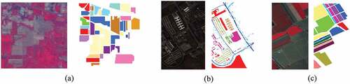
Three data sets were tested in this paper: 1) the airborne visible/infrared imaging spectrometer (AVIRIS) Indian Pines data set (Data I); 2) the reflective optics system imaging spectrometer (ROSIS) University of Pavia data set (Data II); and 3) the AVIRIS Salinas data set (Data III). The information about the data sets is summarized below:

Data I has a spatial resolution of 20 m. It consists of 145$\times$145 pixels with 220 spectral bands in the range of 0.4–2.5 $\mu$m. 20 water absorption bands were removed prior to the experiments. Data I contains 16 labeled classes.

Data II consists of 610$\times$340 pixels and nine labeled classes with a spatial resolution of 1.3 m. 103 spectral bands from 0.43 to 0.86 $\mu$m are used in the experiments.

Data III consists of 512 $\times$217 pixels. Each pixel has 204 data channels with 20 bands removed prior to the experiments due to the water absorption. The spatial resolution of this data set is 3.7 m. 16 labeled classes are used as reference in this paper.

In the experiments, the training samples for each class were randomly selected, and the remaining were used as the test set. The class information for the three data sets and the numbers of training and test samples are listed in Tables 1-3, respectively. Figure 2 shows the ground truth and false color images of the data sets.

Table 1. Sixteen ground truth classes and the numbers of training and test samples for Data I.

No.	Class Name	Train	Test
1	Alfalfa	20	26
2	Corn-no till	50	1378
3	Corn-min till	50	780
4	Corn	50	187
5	Grass/pasture	50	433
6	Grass/trees	50	680
7	Grass/pasture-mowed	10	18
8	Hay-windrowed	50	428
9	Oats	10	10
10	Soybeans-no till	50	922
11	Soybeans-min till	50	2405
12	Soybeans-clean till	50	543
13	Wheat	21	184
14	Woods	50	1215
15	Buildings-grass-trees	50	336
16	Stone-steel towers	20	73
Total		631	9618

Table 2. Nine ground truth classes and the numbers of training and test samples for Data II.

No.	Class Name	Train	Test
1	Asphalt	150	6481
2	Meadows	150	18,499
3	Gravel	150	1949
4	Trees	150	2914
5	Meta sheets	150	1195
6	Bare soil	150	4879
7	Bitumen	150	1180
8	Bricks	150	3532
9	Shadows	150	797
Total		1350	41,426

Table 3. Sixteen ground truth classes and the numbers of training and test samples for Data III.

No.	Class Name	Train	Test
1	Weeds_1	100	1909
2	Weeds_2	100	3626
3	Fallow	100	1876
4	Fallow plow	100	1294
5	Fallow smooth	100	2578
6	Stubble	100	3859
7	Celery	100	3479
8	Grapes	100	11,171
9	Soil	100	6103
10	Corn	100	3178
11	Lettuce 4 week	100	968
12	Lettuce 5 week	100	1827
13	Lettuce 6 week	100	816
14	Lettuce 7 week	100	970
15	Vineyard untrained	100	7168
16	Vineyard trellis	100	1707
Total		1600	52,529

Figure 2. False color composite image with bands 50–27-17 (left) and ground truth (right) for three data sets: (a) Data I; (b) Data II; (c) Data III.

3.2. Experimental setting

The proposed framework is compared with several spectral-spatial methods to evaluate the performance. SVM with extended multi-attribute profiles (EMAP) (referred to as SVM-EMAP) (Mura et al. 2011), probabilistic SVM with MRF (referred to as SVM-MRF), JSM with SOMP (referred to as JSM) (Chen, Nasrabadi, and Tran 2011), probabilistic SR with MRF (referred to as SR-MRF), and probabilistic JSM with MRF (referred to as JSM-MRF) are used as the benchmarks. SVM was implemented using the libsvm library with the Gaussian kernel (Chang and Lin 2011). The spatial information for SVM-EMAP features was extracted by the technique presented in (Dalla Mura et al. 2011). The sparsity level $K$ was set as 3 for all three data sets as suggested in (Chen, Nasrabadi, and Tran 2011; Ghamisi et al. 2018). The optimal values for the neighborhood region are set differently for the three data sets (i.e. 7$\times$7 for Data I, 11$\times$11 for Data II, and 15$\times$15 for Data III) as demonstrated in (Gao, Lim, and Jia 2018b). The weight parameter was set to 0.2, 0.3 and 0.6 for the three data sets from cross-validation using the leave-one-out strategy, respectively. Three well-known quantitative metrics, namely overall accuracy (OA), average accuracy (AA) and kappa coefficient (k) are selected for the quantitative validation in this paper. Ten random sampling-based repeated experiments are conducted for each data set.

3.3. Experimental results

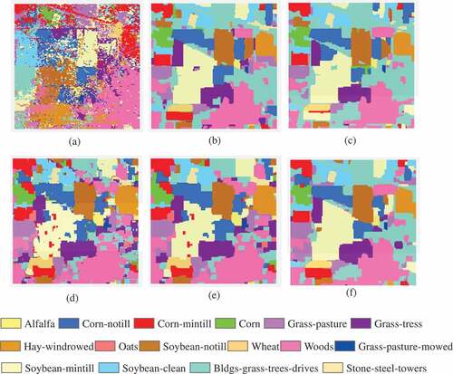
The experimental results for Data I are illustrated in Table 4 and Figure 3. As can be observed from the classification maps in Figure 3, the spectral-spatial classifiers produced relatively smooth and accurate classification results. However, SVM-EMAP and SR-MRF produced comparatively nosily results and failed to detect some meaningful areas, such as the near-boundary regions. Although JSM, SVM-MRF and JSM-MRF performed the classification task reasonably well, noisy appearance is still evident on the classification maps. In contrast, the proposed method reduced the noise and preserved the near-boundary regions. The quantitative results tabulated in Table 4 clearly show that the proposed method outperformed the other classifiers with respect to the three metrics. It can be observed that the accuracy of our method is 1.54% and 4.49% higher than JSM-MRF and SVM-MRF, respectively, which confirms the effectiveness of the proposed fusion strategy.

Table 4. Classification results obtained by different classifiers on Data I for each class.

Class	SVM-EMAP	SVM-MRF	SR-MRF	JSM	JSM-MRF	Proposed
1	73.91	97.83	100.00	100.00	100.00	100.00
2	58.61	76.26	77.31	85.85	89.99	87.11
3	59.28	85.78	59.76	85.78	91.45	91.69
4	65.82	99.16	99.16	99.16	99.58	100.00
5	68.32	95.65	87.58	98.34	98.14	96.48
6	62.74	100.00	98.63	95.89	96.16	99.73
7	71.43	92.86	96.43	85.71	78.57	100.00
8	85.36	100.00	98.95	98.54	100.00	100.00
9	75.00	100.00	100.00	90.00	80.00	100.00
10	66.56	87.96	92.18	91.67	92.18	89.71
11	53.24	82.04	73.77	85.74	85.25	90.55
12	73.69	91.91	98.65	83.47	89.54	97.47
13	73.66	99.51	99.51	94.15	99.02	99.51
14	79.29	96.21	90.43	95.42	94.07	95.49
15	83.16	97.93	100.00	93.26	98.96	99.74
16	21.51	100.00	100.00	90.32	98.92	98.90
OA (%)	64.75	88.82	84.53	90.17	91.77	93.31
AA (%)	66.97	93.94	92.02	92.08	93.24	96.65
k	0.61	0.88	0.83	0.89	0.91	0.92

Figure 3. Classification maps obtained by different classifiers for Data I with 16 classes: (a) SVM-EMAP; (b) SVM-MRF; (C) SR-MRF; (d) JSM; (e) JSM-MRF; (f) Proposed.

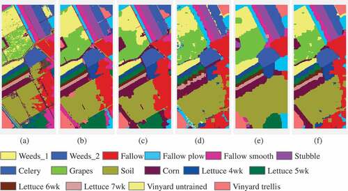
The classification results on the other two data sets are shown in Table 5-6 and Figure 4–5, respectively. Compared with SVM-MRF and JSM-MRF, our method improved the overall accuracy up to 12.30% and 2.17% for Data II, and 1.92% and 0.4% for Data III, respectively. The visual inspection from the classification maps is consistent with the resultant tables. The fusion strategy smoothed the classification maps, however, it tends to over-smooth some of the boundary lines within each classified region, which can also be observed from the classification maps. It also should be noticed that there are still some small misclassified patches because of the limited number of training samples.

Table 5. Classification results obtained by different classifiers on Data II for each class.

Class	SVM-EMAP	SVM-MRF	SR-MRF	JSM	JSM-MRF	Proposed
1	83.15	98.30	97.32	82.82	91.10	96.46
2	85.20	70.61	61.87	91.29	98.54	98.94
3	74.27	79.37	92.90	87.47	94.62	93.28
4	95.63	98.56	98.63	95.69	78.85	89.85
5	98.36	99.85	99.93	99.63	99.78	100.00
6	88.92	98.47	98.95	92.60	100.00	100.00
7	90.75	95.64	96.24	93.76	99.10	99.40
8	77.81	97.77	97.53	85.82	98.34	98.48
9	97.99	99.26	99.79	99.89	72.02	90.92
OA (%)	85.77	85.28	82.06	90.32	95.41	97.58
AA (%)	88.01	93.09	93.68	92.11	92.48	96.37
k	0.82	0.82	0.78	0.87	0.94	0.97

Table 6. Classification results obtained by different classifiers on Data III for each class.

Class	SVM-EMAP	SVM-MRF	SR-MRF	JSM	JSM-MRF	Proposed
1	99.45	100.00	100.00	96.27	100.00	100.00
2	99.60	100.00	99.81	98.85	99.95	99.79
3	98.23	99.80	100.00	100.00	100.00	99.95
4	97.06	100.00	99.64	93.33	99.78	99.71
5	96.60	98.47	98.36	94.88	99.37	99.22
6	99.85	100.00	100.00	94.06	99.90	99.90
7	99.75	99.72	99.83	92.12	99.66	99.69
8	68.73	90.53	75.66	91.30	90.49	91.36
9	99.58	99.11	99.58	99.81	99.66	99.65
10	95.55	97.07	95.85	86.97	97.50	98.41
11	97.94	98.78	94.66	96.16	99.72	99.72
12	100.00	99.95	100.00	99.27	100.00	100.00
13	98.47	99.45	99.45	98.14	99.13	99.02
14	98.32	99.81	97.76	99.07	99.91	99.91
15	92.71	81.37	82.77	92.53	92.17	93.37
16	100.00	100.00	98.34	97.40	98.40	99.17
OA (%)	91.71	95.11	91.99	94.54	96.63	97.03
AA (%)	96.36	97.75	96.36	95.63	98.48	98.68
k	0.91	0.95	0.91	0.94	0.96	0.97

Figure 5. Classification maps obtained by different classifiers for Data III with 16 classes: (a) SVM-EMAP; (b) SVM-MRF; (C) SR-MRF; (d) JSM; (e) JSM-MRF.

3.4. Discussion

It is more sensible to compare the results obtained by SVM-MRF, SR-MRF, JSM-MRF and the proposed method, because they are all MRF-based probabilistic methods. Moreover, SVM-MRF performed better than SR-MRF which can be observed from the resultant tables. All in all, the proposed method achieved the highest accuracy on all three benchmark data sets with respect to the widely used quantitative metrics. Table 4-6 show that the results obtained by other classifiers vary from classifier to classifier and from data set to data set, and one can conclude from the results that the proposed method is highly reliable and stable regardless of data sets.

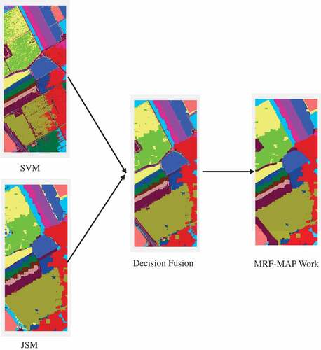
In order to help understanding of the scheme of the proposed framework, Figure 6-8 illustrate the maps after each step i.e. SVM, JSM, decision fusion and the MRF-MAP work for the three data sets. It can be observed that the maps obtained by SVM are more noisy due to the lack of consideration of spatial information, while the ones obtained by JSM are smoother. However, due to the over-smoothing effect, the classification maps by JSM in near-edge areas are blurred. Although the classification maps after decision fusion have more scattered points than JSM in homogenous areas, the near-edge areas are clearly refined. Therefore, the MRF-MAP work can be effectively used to refine the results in homogenous areas and obtain a more accurate classification map for the whole area.

Figure 6. Classification maps of Data I after SVM, JSM and fusion.

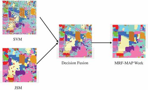
Figure 8. Classification maps of Data III after SVM, JSM and fusion.

The proposed method eliminates the noise and enhances the results from SVM and JSM via the fusion strategy. These aspects together with the joint characterization of spatial-contextual information by MRF-MAP make the framework prominent in integrating local and global probabilities. To draw a conclusion, the proposed method delivers more uniform results. When compared to the results in (Li et al. 2015; Chen, Nasrabadi, and Tran 2011), the proposed method shows consistently better performance for the three data sets. The fusion method takes the advantages of both SVM and JSM and can overcome the situation in which one of the methods does not provide good performance. This is also the reason why the proposed method can provide better performance than the comparative classifiers.

3.5. Impact of parameters

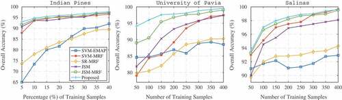
This section explores the impact of training samples on the experimental results. To minimize possible sampling bias, the experiments were run ten times repeatedly with randomly chosen training samples each time. The OA values under different conditions of training numbers are evaluated. For Data I, 5% to 40% of the total samples were used as training samples. For Data II and Data III, the number of training samples varies from 50 to 400. The remaining is used as test sets. Figure 9 depicts the results for different classification approaches with different numbers of training samples. As can be observed from the figure, the performances of SVM-EMAP, SVM-MRF, SR-MRF, JSM, JSM-MRF and the proposed methods generally improve as the numbers of training samples increase. SVM-EMAP shows the least stability with some small fluctuations in the experiments. It can be also seen that SVM-MRF performs better on Indian Pines than the other two data sets, and this may be due to the fact that the mixed pixels present in this data set are more helpful in the class discrimination of SVM-MRF. JSM-MRF can achieve a very high accuracy for all three data sets with an adequate number of training samples, and it benefits from the spatial information being considered in both the probabilistic classification and post-processing. In addition, the proposed classifier can consistently achieve the best results on all training samples. The trends observed from Figure 9 also confirm that our method is working effectively even if a small number of training samples are available, which is very promising for practical applications.

Figure 9. The impact of training samples on OA results of the test methods for three test data sets.

4. Conclusion

We proposed a novel framework which integrates the SVM and JSM methods in a probabilistic sense for HSI classification. The proposed framework focuses on different contributions of the two methods. SVM is used to obtain the global probability distribution for all pixels, and JSM is used to determine better representation of test pixels than the common SR-based methods by exploiting the spatial correlations among neighboring pixels. In this paper, JSM is applied to compute the reconstruction errors of different classes, and then the posterior probability distributions corresponding to the different classes are obtained by an inverse formula of the reconstruction errors. Under the assumption of the independence of each class, the posterior probabilities are used as prior label probability distributions in MRF, and the final labels are derived by solving a MAP problem. The proposed framework maintains the complementary information of different techniques and keeps the spatial smoothness of the images. The validation on three benchmark data sets shows that the proposed method yielded a very high accuracy, even though a smaller number of training samples are used.

Highlights

• We developed and applied a new framework for HSI classification.

• The new method consists of a SVM, a JSM and a MRF.

• The results of SVM and JSM are fused by a linear opinion pool.

• A MRF is applied to regularize the final results.

• The proposed method performs very well with limited training samples.

Acknowledgements

The authors would like to thank Prof. D. Landgrebe from Purdue University, for providing the free downloads of the hyperspectral AVIRIS data set, Prof. Paolo Gamba from the Telecommunications and Remote Sensing Laboratory for providing the Pavia University data set, the California Institute of Technology for providing the Salinas data set. The authors would like to thank the Associate Editor and anonymous reviewers for their careful reading and valuable comments which were very helpful to improve this paper.

Disclosure statement

No potential conflict of interest was reported by the authors.

References

- Boykov, Y., and V. Kolmogorov. 2004. “An Experimental Comparison of Min-Cut/Max-Flow Algorithms for Energy Minimization in Vision.” IEEE Transactions on Pattern Analysis and Machine Intelligence 26 (9): 1124–1137. doi:10.1109/TPAMI.2004.60.
- Campbell, J. B., and R. H. Wynne. 2011. Introduction to Remote Sensing. New York, NY: Guilford Press.
- Cao, X., X. Lin, D. Meng, Q. Zhao, and X. Zongben. 2017. “Integration of 3-Dimensional Discrete Wavelet Transform and Markov Random Field for Hyperspectral Image Classification.” Neurocomputing 226: 90–100. doi:10.1016/j.neucom.2016.11.034.
- Carvalho, A., and K. Larson. 2013. “A Consensual Linear Opinion Pool.” Paper presented at the IJCAI, Beijing, China.
- Chang, C.-C., and C.-J. Lin. 2011. “LIBSVM: A Library for Support Vector Machines.” ACM Transactions on Intelligent Systems and Technology (TIST) 2 (3): 27.
- Chen, Y., N. M. Nasrabadi, and T. D. Tran. 2011. “Hyperspectral Image Classification Using Dictionary-Based Sparse Representation.” IEEE Transactions on Geoscience and Remote Sensing 49 (10): 3973–3985. doi:10.1109/TGRS.2011.2129595.
- Chen, Y., N. M. Nasrabadi, and T. D. Tran. 2013. “Hyperspectral Image Classification via Kernel Sparse Representation.” IEEE Transactions on Geoscience and Remote Sensing 51 (1): 217–231. doi:10.1109/TGRS.2012.2201730.
- Chu, H.-J., C.-K. Wang, S.-J. Kong, and K.-C. Chen. 2016. “Integration of Full-Waveform LiDAR and Hyperspectral Data to Enhance Tea and Areca Classification.” GIScience & Remote Sensing 53 (4): 542–559. doi:10.1080/15481603.2016.1177249.
- Fang, L., L. Shutao, X. Kang, and J. A. Benediktsson. 2014. “Spectral–Spatial Hyperspectral Image Classification via Multiscale Adaptive Sparse Representation.” IEEE Transactions on Geoscience and Remote Sensing 52 (12): 7738–7749. doi:10.1109/TGRS.2014.2318058.
- Fu, W., L. Shutao, L. Fang, and J. A. Benediktsson. 2017. “Adaptive Spectral–Spatial Compression of Hyperspectral Image with Sparse Representation.” IEEE Transactions on Geoscience and Remote Sensing 55 (2): 671–682. doi:10.1109/TGRS.2016.2613848.
- Gao, L., L. Jun, M. Khodadadzadeh, A. Plaza, B. Zhang, H. Zhijian, and H. Yan. 2015. “Subspace-Based Support Vector Machines for Hyperspectral Image Classification.” IEEE Geoscience and Remote Sensing Letters 12 (2): 349–353. doi:10.1109/LGRS.2014.2341044.
- Gao, Q., S. Lim, and X. Jia. 2018a. “Hyperspectral Image Classification Using Joint Sparse Model and Discontinuity Preserving Relaxation.” IEEE Geoscience and Remote Sensing Letters 15 (1): 78–82. doi:10.1109/LGRS.2017.2774253.
- Gao, Q., S. Lim, and X. Jia. 2018b. “Improved Joint Sparse Models for Hyperspectral Image Classification Based on a Novel Neighbour Selection Strategy.” Remote Sensing 10 (6): 905. doi:10.3390/rs10060905.
- Ghamisi, P., E. Maggiori, L. Shutao, R. Souza, Y. Tarablaka, G. Moser, A. De Giorgi, L. Fang, Y. Chen, and M. Chi. 2018. “New Frontiers in Spectral-Spatial Hyperspectral Image Classification: The Latest Advances Based on Mathematical Morphology, Markov Random Fields, Segmentation, Sparse Representation, and Deep Learning.” IEEE Geoscience and Remote Sensing Magazine 6 (3): 10–43. doi:10.1109/MGRS.2018.2854840.
- Gualtieri, J. A., and R. F. Cromp. 1999. “Support Vector Machines for Hyperspectral Remote Sensing Classification.” Paper presented at the 27th AIPR Workshop: Advances in Computer-Assisted Recognition, Washington, DC.
- Ham, J., Y. Chen, M. M. Crawford, and J. Ghosh. 2005. “Investigation of the Random Forest Framework for Classification of Hyperspectral Data.” IEEE Transactions on Geoscience and Remote Sensing 43 (3): 492–501. doi:10.1109/TGRS.2004.842481.
- Huang, C., L. S. Davis, and J. R. G. Townshend. 2002. “An Assessment of Support Vector Machines for Land Cover Classification.” International Journal of Remote Sensing 23 (4): 725–749. doi:10.1080/01431160110040323.
- Jia, X., C. Dey, D. Fraser, L. Lymburner, and A. Lewis. 2010. “Controlled Spectral Unmixing Using Extended Support Vector Machines.” Paper presented at the Hyperspectral Image and Signal Processing: Evolution in Remote Sensing (WHISPERS), Reykjavik, Iceland, 2010 2nd Workshop.
- Juan, O., and Y. Boykov. 2007. “Capacity scaling for graph cuts in vision.” .
- Kolmogorov, V., and R. Zabin. 2004. “What Energy Functions Can Be Minimized via Graph Cuts?” IEEE Transactions on Pattern Analysis and Machine Intelligence 26 (2): 147–159. doi:10.1109/TPAMI.2004.1262177.
- Landgrebe, D. A. 2005. Signal Theory Methods in Multispectral Remote Sensing. Vol. 29. Milton QLD, Australia: John Wiley & Sons.
- Li, J., H. Zhang, and L. Zhang. 2014. “Supervised Segmentation of Very High Resolution Images by the Use of Extended Morphological Attribute Profiles and a Sparse Transform.” IEEE Geoscience and Remote Sensing Letters 11 (8): 1409–1413. doi:10.1109/LGRS.2013.2294241.
- Li, J., J. M. Bioucas-Dias, and A. Plaza. 2012. “Spectral–Spatial Hyperspectral Image Segmentation Using Subspace Multinomial Logistic Regression and Markov Random Fields.” IEEE Transactions on Geoscience and Remote Sensing 50 (3): 809–823. doi:10.1109/TGRS.2011.2162649.
- Li, J., J. M. Bioucas-Dias, and A. Plaza. 2013. “Semisupervised Hyperspectral Image Classification Using Soft Sparse Multinomial Logistic Regression.” IEEE Geoscience and Remote Sensing Letters 10 (2): 318–322. doi:10.1109/LGRS.2012.2205216.
- Li, J., X. Huang, P. Gamba, J. M. Bioucas-Dias, L. Zhang, J. A. Benediktsson, and A. Plaza. 2015. “Multiple Feature Learning for Hyperspectral Image Classification.” IEEE Transactions on Geoscience and Remote Sensing 53 (3): 1592–1606. doi:10.1109/TGRS.2014.2345739.
- Lin, Z., and L. Yan. 2016. “A Support Vector Machine Classifier Based on A New Kernel Function Model for Hyperspectral Data.” GIScience & Remote Sensing 53 (1): 85–101. doi:10.1080/15481603.2015.1114199.
- Melgani, F., and L. Bruzzone. 2004. “Classification of Hyperspectral Remote Sensing Images with Support Vector Machines.” IEEE Transactions on Geoscience and Remote Sensing 42 (8): 1778–1790. doi:10.1109/TGRS.2004.831865.
- Moser, G., and S. B. Serpico. 2013. “Combining Support Vector Machines and Markov Random Fields in an Integrated Framework for Contextual Image Classification.” IEEE Transactions on Geoscience and Remote Sensing 51 (5): 2734–2752. doi:10.1109/TGRS.2012.2211882.
- Mountrakis, G., J. Im, and C. Ogole. 2011. “Support Vector Machines in Remote Sensing: A Review.” ISPRS Journal of Photogrammetry and Remote Sensing 66 (3): 247–259. doi:10.1016/j.isprsjprs.2010.11.001.
- Mura, D., A. V. Mauro, J. A. Benediktsson, J. Chanussot, and L. Bruzzone. 2011. “Classification of Hyperspectral Images by Using Extended Morphological Attribute Profiles and Independent Component Analysis.” IEEE Geoscience and Remote Sensing Letters 8 (3): 542–546. doi:10.1109/LGRS.2010.2091253.
- Plaza, A., J. A. Benediktsson, J. W. Boardman, J. Brazile, L. Bruzzone, G. Camps-Valls, J. Chanussot, M. Fauvel, P. Gamba, and A. Gualtieri. 2009. “Recent Advances in Techniques for Hyperspectral Image Processing.” Remote Sensing of Environment 113: S110–S22. doi:10.1016/j.rse.2007.07.028.
- Ratle, F., G. Camps-Valls, and J. Weston. 2010. “Semisupervised Neural Networks for Efficient Hyperspectral Image Classification.” IEEE Transactions on Geoscience and Remote Sensing 48 (5): 2271–2282. doi:10.1109/TGRS.2009.2037898.
- Srinivas, U., Y. Chen, V. Monga, N. M. Nasrabadi, and T. D. Tran. 2013. “Exploiting Sparsity in Hyperspectral Image Classification via Graphical Models.” IEEE Geoscience and Remote Sensing Letters 10 (3): 505–509. doi:10.1109/LGRS.2012.2211858.
- Tarabalka, Y., M. Fauvel, J. Chanussot, and J. A. Benediktsson. 2010. “SVM-and MRF-based Method for Accurate Classification of Hyperspectral Images.” IEEE Geoscience and Remote Sensing Letters 7 (4): 736–740. doi:10.1109/LGRS.2010.2047711.
- Tesfamichael, S. G., S. W. Newete, E. Adam, and B. Dubula. 2018. “Field Spectroradiometer and Simulated Multispectral Bands for Discriminating Invasive Species from Morphologically Similar Cohabitant Plants.” GIScience & Remote Sensing 55 (3): 417–436. doi:10.1080/15481603.2017.1396658.
- Tu, B., S. Huang, L. Fang, G. Zhang, J. Wang, and B. Zheng. 2018a. “Hyperspectral Image Classification via Weighted Joint Nearest Neighbor and Sparse Representation.” IEEE Journal of Selected Topics in Applied Earth Observations and Remote Sensing,11 (11): 4063–4075.
- Tu, B., X. Zhang, X. Kang, G. Zhang, J. Wang, and W. Jianhui. 2018b. “Hyperspectral Image Classification via Fusing Correlation Coefficient and Joint Sparse Representation.” IEEE Geoscience and Remote Sensing Letters 15 (3): 340–344. doi:10.1109/LGRS.2017.2787338.
- Villa, A., J. Chanussot, J. A. Benediktsson, and C. Jutten. 2011. “Spectral Unmixing for the Classification of Hyperspectral Images at a Finer Spatial Resolution.” IEEE Journal of Selected Topics in Signal Processing 5 (3): 521–533. doi:10.1109/JSTSP.2010.2096798.
- Xu, L., and J. Li. 2014. “Bayesian Classification of Hyperspectral Imagery Based on Probabilistic Sparse Representation and Markov Random Field.” IEEE Geoscience and Remote Sensing Letters 11 (4): 823–827. doi:10.1109/LGRS.2013.2279395.
- Xun, L., and L. Wang. 2015. “An Object-Based SVM Method Incorporating Optimal Segmentation Scale Estimation Using Bhattacharyya Distance for Mapping Salt Cedar (Tamarisk Spp.) With QuickBird Imagery.” GIScience & Remote Sensing 52 (3): 257–273. doi:10.1080/15481603.2015.1026049.
- Zhang, C., M. Smith, and C. Fang. 2018. “Evaluation of Goddard’s LiDAR, Hyperspectral, and Thermal Data Products for Mapping Urban Land-Cover Types.” GIScience & Remote Sensing 55 (1): 90–109. doi:10.1080/15481603.2017.1364837.
- Zhang, X., Z. Gao, L. Jiao, and H. Zhou. 2018. “Multifeature Hyperspectral Image Classification with Local and Nonlocal Spatial Information via Markov Random Field in Semantic Space.” IEEE Transactions on Geoscience and Remote Sensing 56 (3): 1409–1424. doi:10.1109/TGRS.2017.2762593.